Dynamics in Stationary, Non-Globally-Hyperbolic Spacetimes

Abstract

Classically, the dynamics of a scalar field in a non-globally-hyperbolic spacetime is ill posed. Previously, a prescription was given for defining dynamics in static spacetimes in terms of a second-order operator acting on a Hilbert space defined on static slices. The present work extends this result by giving a similar prescription for defining dynamics in stationary spacetimes obeying certain mild assumptions. The prescription is defined in terms of a first-order operator acting on a different Hilbert space from the one used in the static prescription. It preserves the important properties of the earlier prescription: the formal solution agrees with the Cauchy evolution within the domain of dependence, and smooth data of compact support always give rise to smooth solutions. In the static case, the first-order formalism agrees with second-order formalism (using specifically the Friedrichs extension). Applications to field quantization are also discussed.

1 Introduction

Let $(M,g_{ab})$ be a spacetime, and consider the minimally coupled, massive Klein-Gordon equation for a real scalar field in this spacetime:

$$(g^{ab}\nabla_{a}\nabla_{b}-m^{2})\varphi=0.$$ (1.1)

As is well known (see, e.g., [1]), if $(M,g_{ab})$ is globally hyperbolic, the Klein-Gordon equation is well posed. That is, given smooth data on a spatial (Cauchy) hypersurface $\Sigma_{0}$, there exists a unique smooth solution $\varphi:M\rightarrow\mathbb{R}$ with the given initial data. In a non-globally-hyperbolic spacetime, however, no similar result holds. It is possible that no solution exists to given initial data, or, if solutions exist, there may be many which satisfy the initial condition. On the other hand, an analysis of Einstein’s equation led Penrose to his “strong” cosmic censorship conjecture [2], which postulates that all “reasonable” spacetimes are globally hyperbolic. For these reasons, the study of dynamics has often been restricted to globally hyperbolic spacetimes.

In the absence of strong evidence either for or against cosmic censorship, Wald [3] considered whether a sensible prescription could be given to define dynamics in a non-globally-hyperbolic spacetime. He studied stably causal, static spacetimes, that is, spacetimes with a hypersurface orthogonal Killing vector field, whose orbits are complete and everywhere timelike. In these spacetimes, the Klein-Gordon equation can be split into its spatial and temporal parts, leading to a second-order equation:

$$\frac{\partial^{2}\phi}{\partial t^{2}}=-A\phi~{}~{}~{}~{}~{}~{}~{}~{}A:=-\alpha D^{a}(\alpha D_{a})+\alpha^{2}m^{2},$$ (1.2)

where $\alpha$ denotes the norm of the Killing field and $D_{a}$ the spatial covariant derivative. The operator $A$ is a positive symmetric operator on an appropriate Hilbert space of initial data. Thus, at least one self-adjoint extension, the Friedrichs extension, always exists [4]. The standard calculus of self-adjoint operators (see, e.g., [5, 6]) can therefore be used to define a solution

$$\phi_{t}=\cos\left(A_{E}^{\frac{1}{2}}t\right)\phi_{0}+A_{E}^{-\frac{1}{2}}\sin\left(A_{E}^{\frac{1}{2}}t\right)(\alpha\pi_{0}),$$ (1.3)

where $A_{E}$ denotes some self-adjoint extension of $A$ (not necessearily the Friedrichs extension $A_{F}$), $\phi_{0}$ the initial field configuration, and $\pi_{0}$ the initial canonical momentum (the canonical momentum is $\pi=n^{a}\nabla_{a}\phi,$ where $n_{a}$ denotes the unit normal to the static slices). For initial data in $C_{0}^{\infty}$, this solution is smooth throughout spacetime, agrees with the classical solution within the domain of dependence $D(\Sigma_{0})$, and solves the Klein-Gordon equation in the pointwise (spacetime) sense. Thus, the map $(\phi_{0},\pi_{0})\rightarrow\phi_{t}$ assigns to each initial datum pair a unique solution with sensible properties, and thus gives rise to a reasonable prescription in the sense defined by Wald and Ishibashi [7]. Indeed, [7] establishes that any reasonable prescription must correspond to the one above for some choice of positive, self-adjoint extension $A_{E}$. In this sense, the choice of extension encodes the “boundary conditions at the singularity” (or whatever feature gives rise to the non-globally-hyperbolicity).

This paper is concerned with a similar prescription for stably casual, stationary spacetimes, i.e., those which possess a complete 1-parameter family of timelike symmetries whose orbits are not necessarily hypersurface orthogonal. In this case, there are “mixed space-time derivatives” in the Klein-Gordon equation, so the division into space and time parts of the equation that was done in (1.2) is no longer possible. However, following Kay [8] by rewriting the Klein-Gordon equation in Hamiltonian form and using an “energy-norm” Hilbert space, the time-evolution operator can be made into a skew-symmetric operator. When this operator can be extended to a skew-adjoint operator, a prescription analogous to (1.3) can be given.

In contrast to the static case, it is not known a priori that any skew-adjoint extension of the time-evolution operator exists. However, if the Killing field does not approach a null vector (in a precise sense explained further in Section 3), it is possible to show that skew-adjoint extensions exist when fields with positive mass are considered. Under these same conditions, this prescription preserves the important properties of the second-order prescription: it agrees with the differential equation within the domain of dependence, and smooth data of compact support give rise to smooth solutions. Further, in the static case it is possible to compare the first and second-order formalisms and show that they agree so long as the Freidrichs extension $A_{F}$ is used in (1.3). An interesting contrast between the first and second-order formalisms becomes apparent during this analysis. In the second-order formalism, a single Hilbert space can be used to define all reasonable dynamics, and the “boundary conditions at the singularity” are determined by the choice of self-adjoint extension. In order to handle different boundary conditions, the first-order formalism must be modified to allow for different Hilbert spaces. Within each one, there is only one skew-adjoint extension of the time-evolution operator. Hence the choice of Hilbert space, not of skew-adjoint extension, determines the dynamics and thus encodes the boundary conditions.

This paper is organized as follows: Section 2 reviews the theory of self-adjoint extensions of symmetric operators and proves a corresponding result regarding skew-adjoint extensions of skew-symmetric operators. Section 3 introduces the prescription in detail. In Section 4, it is shown that skew-adjoint extensions of the time-evolution operator exist. It is further shown that the prescription agrees with the differential equation within the domain of dependence and that smooth data of compact support give rise to smooth solutions. Section 5 examines the static case and compares the first and second-order formalisms. As defining the space of classical solutions is the first step towards field quantization, Section 6 show how this prescritption may be used to extend the well-known constructions of globally hyperbolic spacetimes to non-globally-hyperbolic ones. Section 7 concludes with some open problems.

2 Extensions of Operators

Although it is common in the physics literature to treat symmetric operators (also called Hermitian operators) as equivalent to self-adjoint operators, these two classes are in fact distinct. The key difference is that arbitrary functions (and, in particular, the exponential) of self-adjoint operators may be defined, whereas this is not true of a general symmetric operator. The reason for this difference is that the proper definition of an operator involves not only specifying its action on vectors but also its domain. A symmetric operator $A$ on a Hilbert space $\mathcal{H}$ is a linear operator defined on a dense vector subspace $\mathrm{Dom}\ A\subseteq\mathcal{H}$, which “acts the same to the left or to the right” for all vectors in its domain:

$$\left<\chi\left.\vphantom{\chi}\vphantom{A\psi}\right|A\psi\right>=\left<A\chi\left.\vphantom{A\chi}\vphantom{\psi}\right|\psi\right>~{}\forall~{}\psi,\chi\in\mathrm{Dom}\ A.$$

A self-adjoint operator is a symmetric operator whose domain is equal to the domain of its adjoint. While $\mathrm{Dom}\ A$ may be freely chosen provided it is a dense vector subspace of $\mathcal{H}$, the domain of $A^{*}$ is fixed once $A$ is defined. The somewhat convoluted definition is as follows: $u\in\mathrm{Dom}\ A^{*}$ if and only if $\exists v\in\mathcal{H}$ such that

$$\left<u\left.\vphantom{u}\vphantom{A\psi}\right|A\psi\right>=\left<v\left.\vphantom{v}\vphantom{\psi}\right|\psi\right>~{}\forall~{}\psi\in\mathrm{Dom}~{}A,$$

in which case $A^{*}u=v.$ Notice that for a symmetric operator, $\mathrm{Dom}\ A$ is automatically contained in $\mathrm{Dom}\ A^{*}$, so if the domains are not equal then $\mathrm{Dom}\ A\subsetneq\mathrm{Dom}\ A^{*}$. The equality of domains for self-adjoint operators is crucial to the proof of the spectral theorem, which allows arbitrary (measurable) functions of the operator to be defined. For a (closed,) symmetric, non-self-adjoint operator, functions may only be defined by a power series, but this series will always diverge unless it has a finite number of terms.

The close relationship between symmetric and self-adjoint operators suggests that a symmetric operator can be turned into self-adjoint operator by enlarging its domain of definition. That this is often the case for operators acting on a complex Hilbert space is a consequence of a famous theorem of von Neumann [9, 4].

Theorem 2.1

Let $\mathcal{H}$ be a Hilbert space over $\mathbb{C}$ and $A:\mathcal{H}\rightarrow\mathcal{H}$ a symmetric operator. Let $K_{\pm}:=\mathrm{Ker}\left(A^{*}\mp i\right)$, and define $n_{\pm}:=\mathrm{Dim}\ K_{\pm}$. Self-adjoint extensions of $A$ exist if and only if $n_{+}=n_{-}=:n$, in which case they are parametrized by the group $U(n)$.

The indices $n_{\pm}$ are called the deficiency indices. If $n_{\pm}=0$, there is a unique self-adjoint extension and $A$ is called essentially self-adjoint. A standard technique for proving that the deficiency indices are equal is the use of a complex conjugation operator. Any involution (i.e., an operator whose square is the identity) $C$ is called a complex conjugation if it is antilinear and norm preserving. Suppose that $\chi_{\pm}\in\mathcal{H}$ obeys $A^{*}\chi_{\pm}=\pm i\chi_{\pm}$. Assume further that $\exists$ some complex conjugation operator $C$ which commutes with $A$. For any operator $A$, not necessarily symmetric, $[A,C]=0$ implies that $[A^{*},C]=0$ [10, p. 360]. Thus, it follows that $A^{*}C\chi_{\pm}=\mp iC\chi_{\pm}$; that is, $C$ establishes an isomorphism between $K_{+}$ and $K_{-}$ so that the deficiency indices are equal. Von Neumann also proved an extension of this result [9, 10].

Theorem 2.2

Let $\mathcal{H}$ be a Hilbert space over $\mathbb{C}$ and $A:\mathcal{H}\rightarrow\mathcal{H}$ a symmetric operator. If $\ \exists$ a complex conjugation $C:\mathcal{H}\rightarrow\mathcal{H}$ with $[A,C]=0$, then (i) $A$ has self-adjoint extensions, and (ii) $\exists$ self-adjoint extensions of $A$ with $C$-invariant domain.

The previous two theorems only apply to complex Hilbert spaces. However, the theory of extensions on a real Hilbert space is naturally related to the theory on complex spaces by the following proposition.

Proposition 2.1

Let $\mathcal{H}_{\mathbb{R}}$ be a Hilbert space over $\mathbb{R}$, $A:\mathcal{H}_{\mathbb{R}}\rightarrow\mathcal{H}_{\mathbb{R}}$ a symmetric operator, and $A^{\mathbb{C}}$ the corresponding operator acting on $\mathcal{H}_{\mathbb{R}}\otimes\mathbb{C}.$ The self-adjoint extensions of $A$ are in 1-1 correspondence with those self-adjoint extensions of $A^{\mathbb{C}}$ whose domain is invariant under $\mathcal{C}$, the natural complex conjugation operator defined on $\mathcal{H}_{\mathbb{R}}\otimes\mathbb{C}$.

This result is implicit in the original work of von Neumann and Stone [10, Theorems 8.1 and 9.14]. Since $A^{\mathbb{C}}$ obviously commutes with $\mathcal{C}$, parts (i) and (ii) of Theorem 2.2 combined with Proposition 2.1 trivially show:

Proposition 2.2

Let $\mathcal{H}_{\mathbb{R}}$ be a Hilbert space over $\mathbb{R}$. Any symmetric operator $A:\mathcal{H}_{\mathbb{R}}\rightarrow\mathcal{H}_{\mathbb{R}}$ has self-adjoint extensions.

In his original work [3], Wald used the positivity of the operator $A$ in (1.2) to assert the existence of self-adjoint extensions. However, Proposition 2.2 shows that this was unnecessary. Existence follows directly from the fact that $A$ is a symmetric operator defined on a real Hilbert space.

The operator considered in the present work is not symmetric but rather skew-symmetric (or anti-Hermitian). Skew-symmetric operators share many properties of symmetric operators, but pick up a minus sign when the operator is transposed from the bra to the ket (or conversely):

$$\left<\chi\left.\vphantom{\chi}\vphantom{A\psi}\right|A\psi\right>=-\left<A\chi\left.\vphantom{A\chi}\vphantom{\psi}\right|\psi\right>~{}\forall~{}\psi,\chi\in\mathrm{Dom}\ A.$$

In the case of a complex Hilbert space, there is a one-to-one correspondence between symmetric and skew-symmetric operators because multiplication by $i$ turns one type of operator into the other. Thus, the analogue of Theorem 2.1 is trivial. In the real Hilbert space case there is no such correspondence because multiplication by $i$ is not a well-defined operation. However, the analogue of Proposition 2.1 remains true. The following elementary proof can be easily modified to apply to symmetric operators as well.

Proposition 2.3

Let $\mathcal{H}_{\mathbb{R}}$ be a Hilbert space over $\mathbb{R}$, $A:\mathcal{H}_{\mathbb{R}}\rightarrow\mathcal{H}_{\mathbb{R}}$ a skew-symmetric operator, and $A^{\mathbb{C}}$ the corresponding operator acting on $\mathcal{H}_{\mathbb{R}}\otimes\mathbb{C}.$ The skew-adjoint extensions of $A$ are in 1-1 correspondence with those skew-adjoint extensions of $A^{\mathbb{C}}$ whose domain is invariant under the natural complex conjugation operator $\mathcal{C}$.

Proof. Let $B$ be a skew-adjoint extension of $A.$ By construction, $B^{\mathbb{C}}$ is skew-symmetric and has a $\mathcal{C}$-invariant domain. The obvious “definition chasing” computation shows that $B^{\mathbb{C}}$ is in fact a skew-adjoint extension of $A^{\mathbb{C}}.$

Conversely, let $B^{\mathbb{C}}$ be a skew-adjoint extension of $A^{\mathbb{C}}$ whose domain is invariant under $\mathcal{C}$. First, recall that $[\mathcal{C},\left(A^{\mathbb{C}}\right)^{*}]=0$, and notice that, as in the symmetric case, the skew-symmetry of $A^{\mathbb{C}}$ implies that $\mathrm{Dom}\ B^{\mathbb{C}}\subseteq\mathrm{Dom}\ \left(A^{\mathbb{C}}\right)^{*}$. In other words, $B^{\mathbb{C}}=\left.-\left(A^{\mathbb{C}}\right)^{*}\right|_{\mathrm{Dom}B^{\mathbb{C}}}.$ This, combined with the assumed $\mathcal{C}$-invariance of the domain, establish that $[\mathcal{C},B^{\mathbb{C}}]=0$. Define $B:\mathcal{H}_{\mathbb{R}}\rightarrow\mathcal{H}_{\mathbb{R}},$ with $\mathrm{Dom}\ B=$ $\mathrm{Dom}\ B^{\mathbb{C}}\cap\mathcal{H}_{\mathbb{R}}$, by $Bu=B^{\mathbb{C}}u.$ This operator is well defined because $[\mathcal{C},B^{\mathbb{C}}]=0$, and clearly $B$ extends $A$. Another straightforward computation establishes that $B$ is skew-adjoint. $\blacksquare$

Equivalently, since composition with $i$ does not change the domain, the skew-adjoint extensions of $A$ are in 1-1 correspondence with the self-adjoint extensions of $iA^{\mathbb{C}}$ with $\mathcal{C}$-invariant domain. Here, a key a difference between self-adjoint and skew-adjoint operators arises. Since $iA^{\mathbb{C}}$ anticommutes, rather than commutes, with $\mathcal{C}$, $\mathcal{C}$ relates the spaces $K_{\pm}$ to themselves rather than to each other. Thus, $iA^{\mathbb{C}}$ may not have any self-adjoint extensions. A standard example is the operator $A\psi=-\frac{d}{dx}\psi$ on $\mathrm{Dom}\ A=\mathcal{C}_{0}^{\infty}\left(\mathbb{R}^{+}\right)\subseteq L^{2}\left(\mathbb{R}^{+},\mathbb{R}\right)$. $A$ is skew-symmetric, but $iA^{\mathbb{C}}$ has deficiency indices $n_{+}=0,n_{-}=1$ in $L^{2}\left(\mathbb{R}^{+},\mathbb{C}\right)$, so that $A$ possesses no skew-adjoint extensions. A key step in later sections will be establishing, in Theorem 4.2, that skew-adjoint extensions of the time-evolution operator do indeed exist.

3 The Prescription

Let $(M,g_{ab})$ be a non-globally-hyperbolic, connected, stably causal, stationary spacetime. A crucial property of these spacetimes for this prescription is the following:

Proposition 3.1

If $(M,g_{ab})$ is a connected, stably causal, stationary spacetime, then there exists a smoothly embedded spatial hypersurface $\Sigma_{0}$ which intersects each orbit of the Killing field exactly once.

Proof. Since $(M,g_{ab})$ is stably causal, it posseses a smooth global time function [11], i.e., a function $\tau:M\rightarrow\mathbb{R}$ such that $\nabla^{a}\tau$ is a past directed timelike vector field. Consider $\tau=0$, and without loss of generality take the Killing field $\left(\frac{\partial}{\partial t}\right)^{a}$ to be future directed. As $\nabla^{a}\tau$ is past directed, it follows that $\tau$ is a strictly increasing function on the orbits of $\left(\frac{\partial}{\partial t}\right)^{a}$, and hence no orbit can intersect $\tau=0$ more than once. On the other hand, suppose, to the contrary, that there is some orbit $O$ of $\left(\frac{\partial}{\partial t}\right)^{a}$ which does not intersect $\tau=0$. Again without loss of generality, take $O$ to be entirely to the future of $\tau=0$. Let $B=\dot{I}^{+}(O)$, the boundary of the chronological future of $O$. $B$ is non-empty since the open set $\tau<0$ does not intersect the open set $I^{+}(O)$, and $M$ is connected. Let $\mathcal{I}_{t}$ be the isometry corresponding to flowing each point of $M$ by Killing parameter $t$. Since $\left(\frac{\partial}{\partial t}\right)^{a}$ is complete, $\mathcal{I}_{t}(O)=O\>\forall\>t.$ Furthermore, $\mathcal{I}_{t}\left(I^{+}(O)\right)=I^{+}\left(\mathcal{I}_{t}(O)\right)=I^{+}(O).$ This means that $\mathcal{I}_{t}(B)=B\>\forall\>t$, or, equivalently, that $\left(\frac{\partial}{\partial t}\right)^{a}$ is tangent to $B$. However, $B$, as the boundary of the chronological future of a set, is generated by null geodesics, and so cannot have a timelike tangent vector. Therefore, each orbit of $\left(\frac{\partial}{\partial t}\right)^{a}$ must intersect $\tau=0$ exactly once. $\tau=0$ is also automatically smoothly embedded by the inverse function theorem, so it may be taken to be the surface $\Sigma_{0}$. $\blacksquare$

It may appear that the assumption of stable causality is an overly restrictive causality condition. However, the key property of $M$ from the standpoint of the prescription is the existence of the initial surface $\Sigma_{0}$. Furthermore, any stationary spacetime containing such a surface is automatically stably causal, as the Killing parameter may be used to define a global time function on $M.$ Hence, stable causality is precisely the right causality assumption.

Denote by $\gamma_{ab}$ the Riemannian metric induced by $g_{ab}$ on $\Sigma_{0}$, $(\Sigma,\gamma_{ab})$ the abstract manifold so defined, and $(\Sigma_{t},\gamma_{ab})$ the translation of $\Sigma_{0}$ by Killing parameter $t$ (which need not be related to the time function $\tau$ used to define $\Sigma_{0}$). The lapse function $\alpha$ and shift-vector $\beta^{a}$ of the Killing field $\left(\frac{\partial}{\partial t}\right)^{a}$ with respect to the future directed unit normal $n^{a}$ of $\Sigma_{0}$ in $M$ are defined by

$$\left(\frac{\partial}{\partial t}\right)^{a}=\alpha n^{a}+\beta^{a}.$$

The classical Hamiltonian for a Klein-Gordon field with mass $m$ in this foliation is given by

$$H((\varphi,\pi))=\frac{1}{2}\int_{\Sigma}d\gamma\alpha\left(\left[1-\frac{\beta_{a}\beta^{a}}{\alpha^{2}}\right]\pi^{2}+\gamma^{ab}\left[D_{a}\varphi+\frac{\beta_{a}}{\alpha}\pi\right]\left[D_{b}\varphi+\frac{\beta_{b}}{\alpha}\pi\right]+m^{2}\varphi^{2}\right)$$ (3.1)

on $C_{0}^{\infty}(\Sigma)\oplus C_{0}^{\infty}(\Sigma)$, where $\pi:=n^{a}\nabla_{a}\varphi$ is the canonical momentum, $D_{a}$ is the Levi-Civita connection of $\gamma_{ab}$, and $d\gamma=\sqrt{\det\gamma_{\mu\nu}}dx^{1}dx^{2}dx^{3}$ is the metric volume form. Note that $\beta^{a}$ is tangent to $\Sigma,$ so it can be pulled back to $\Sigma$ and the above formula makes sense. This Hamiltonian may be expressed on $C_{0}^{\infty}(\Sigma)\oplus C_{0}^{\infty}(\Sigma)$ data as

$$H((\varphi,\pi))=\frac{1}{2}\int_{\Sigma}d\gamma\left[\begin{array}[]{cc}\varphi&\pi\end{array}\right]\mathcal{A}\left[\begin{array}[]{c}\varphi\\ \pi\end{array}\right],$$

where $\mathcal{A}$ is the matrix differential operator

$$\mathcal{A}=\left[\begin{array}[]{cc}-(D^{a}\alpha)D_{a}+\alpha(m^{2}-D^{a}D_{a})&-(D_{a}\beta^{a})-\beta^{a}D_{a}\\ \beta^{a}D_{a}&\alpha\end{array}\right].$$ (3.2)

Let $\mathcal{H_{A}}$ be the completion of $C_{0}^{\infty}(\Sigma)\oplus C_{0}^{\infty}(\Sigma)$ in the energy norm

$$\|\Phi\|_{\mathcal{A}}^{2}:=2H(\Phi)=\left<\Phi\left.\vphantom{\Phi}\vphantom{\mathcal{A}\Phi}\right|\mathcal{A}\Phi\right>_{L^{2}(d\gamma)\oplus L^{2}(d\gamma)},~{}~{}~{}~{}\Phi=(\varphi,\pi)\in C_{0}^{\infty}(\Sigma)\oplus C_{0}^{\infty}(\Sigma).$$ (3.3)

Thus, the squared norm of a field configuration is equal to twice its classical energy, justifying the name “energy norm.”

It should be noted that while $\mathcal{H_{A}}$ is a natural choice of Hilbert space associated to the system, other choices are possible. That is, it is possible to define an energy norm which agrees with the above definition on smooth data of compact support but is defined on a larger set of functions. In Section 5, it will be shown that other choices for $\mathcal{H_{A}}$ can be used to define different dynamics, although the definitions of $\mathcal{A}$ and $h$ (below) would then need to be modified somewhat.

Let $j$ be the standard $2\times 2$ symplectic matrix,

$$j:=\left[\begin{array}[]{cc}0&1\\ -1&0\end{array}\right],$$

and let

$$h:=-j\mathcal{A}=\left[\begin{array}[]{cc}-\beta^{a}D_{a}&-\alpha\\ -(D^{a}\alpha)D_{a}+\alpha(m^{2}-D^{a}D_{a})&-(D_{a}\beta^{a})-\beta^{a}D_{a}\end{array}\right].$$ (3.4)

Hamilton’s equations for the scalar field then take the simple form

$$\frac{\partial}{\partial t}\Phi(t)=-h\Phi(t).$$

It is easy to check by partial integration that $h$, defined as a differential operator on $C_{0}^{\infty}(\Sigma)\oplus C_{0}^{\infty}(\Sigma)\subseteq\mathcal{H_{A}}$, is a skew-symmetric operator. Formally, the time-evolution equation may be solved by exponentiating $h$. However, this may not be possible unless $h$ is extended to a skew-adjoint operator $h^{SA}$. Skew-adjoint operators have a spectral decomposition similar to that of symmetric operators (see, e.g., [6, Theorem 13.33]). This may be used to exponentiate $h^{SA}$ and give the solution

$$\Phi_{t}=e^{-h^{SA}t}\Phi_{0}.$$ (3.5)

Equation (3.5) assigns to each vector in $\mathcal{H_{A}}$ a strongly continuous one-parameter family of vectors in $\mathcal{H_{A}}$ which represents a formal solution to the Klein-Gordon equation. However, it is not clear a priori that (I) this one-parameter family defines a smooth function on spacetime for smooth initial data of compact support, or that (II) it solves the Klein-Gordon equation in the pointwise (spacetime) sense when the initial data are sufficiently regular.

In order to make any progress in proving (I) and (II), two technical assumptions are made. It is possible that these assumption are not needed, but the methods of proof used Section 4 break down. The first assumption restricts consideration to the massive Klein-Gordon equation:

$$\textrm{(A)}~{}~{}m^{2}>0.$$

3 guarantees that any $\Phi\in\mathcal{H_{A}}$ is automatically in $H^{1}_{\mathrm{{loc}}}\oplus H^{0}_{\mathrm{{loc}}}$, where $H^{k}_{\mathrm{{loc}}}$ denotes the $k$th local Sobolev space (see, e.g., [4]). This ensures that all the vectors in $\mathcal{H_{A}}$ are functions and not distributions. The second assumption is a condition on $\alpha$ and $\beta$:

$$\textrm{(B)}~{}~{}\alpha-\frac{\beta_{a}\beta^{a}}{\alpha}\geq\epsilon>0.$$

Notice that since $\alpha$ is manifestly positive, this condition implies $\alpha\geq\epsilon$ as well as $\left(\frac{\partial}{\partial t}\right)^{a}\left(\frac{\partial}{\partial t}\right)_{a}=\alpha^{2}-\beta^{2}>\epsilon^{2}>0.$ However, if $\alpha$ diverges then 3 is strictly stronger than the condition that the norm of Killing is bounded away from zero. Also notice that since it involves $\beta^{a}$, 3 is a condition on the slice $\Sigma_{0}$ as well as the Killing field. Roughly speaking, 3 implies that the “Lorentz boost” taking the unit normal $n^{a}$ to $\left(\frac{\partial}{\partial t}\right)^{a}$ is bounded, so that the two vectors do not “approach being null with respect to one another.”

A straightforward computation shows that these two conditions together ensure that $\|\Phi\|_{\mathcal{A}}\geq c\|\Phi\|_{L^{2}(d\gamma)\oplus L^{2}(d\gamma)}$, where $c$ is some constant depending only on $\epsilon$ and $m$. One easy consequence of this inequality is that the symplectic form on smooth, compactly supported functions, defined by

$$\sigma\left(F,G\right):=\left<F\left.\vphantom{F}\vphantom{jG}\right|jG\right>_{L^{2}(d\gamma)\oplus L^{2}(d\gamma)},$$ (3.6)

is a continuous bilinear form on $\mathcal{H_{A}}$, i.e., $\exists$ some constant $c_{\sigma}$ so that $|\sigma(F,G)|\leq c_{\sigma}\|F\|_{\mathcal{A}}\|G\|_{\mathcal{A}}.$ This inequality follows from the fact that $j$ is a bounded operator on $L^{2}(d\gamma)\oplus L^{2}(d\gamma)$ combined with the fact that $\mathcal{A}$-norm bounds $L^{2}(d\gamma)\oplus L^{2}(d\gamma)$-norm, and it means that $\sigma$ extends uniquely to a continuous bilinear form on all of $\mathcal{H_{A}}$. This will be critical in in the analysis of Section 4, which shows that (I) is true and that (II) is true so long as $\Phi_{0}$ is smooth and $\Phi_{0}\in\mathrm{Dom}\ h^{SA}$.

To summarize, the prescription is as follows. First, choose any smoothly embedded spatial hypersurface which intersects each orbit of the Killing vector field exactly once and satisfies 3. Second, define the Hilbert space $\mathcal{H_{A}}$ with the norm given by equations (3.2) and (3.3), as well as the operator $h$ on $C_{0}^{\infty}(\Sigma)\oplus C_{0}^{\infty}(\Sigma)$ by (3.4). Finally, choose an arbitrary skew-adjoint extension of $h$ and assign the solution (3.5) to each initial datum $\Phi_{0}\in\mathcal{H_{A}}$. Naively, then, two arbitrary choices—the choice of initial surface and the choice of skew-adjoint extension—plus a possible third choice, if $\mathcal{H_{A}}$ may be replaced by some larger Hilbert space, are allowed in the prescription. However, as shown in Section 5, $h$ is essentially skew-adjoint in static spacetimes. Even if $h$ is not always essentially skew-adjoint, Theorem 4.2 shows that there is always a preferred skew-adjoint extension. Both these facts suggest that there is considerably less freedom available than at first appears. Finally, whether the prescription gives rise to the same dynamics when inequivalent slicings in the same spacetime are used remains an open question.

4 Properties of the Prescription

The goal of this section is to prove two theorems. The first assumes the existence of skew-adjoint extensions of $h$, and proves that any such extension gives rise to a prescription with reasonable properties. The proof is more or less a direct adaptation of the corresponding theorem in [3]. The second theorem establishes the existence of skew-adjoint extensions as well as a certain preferred extension. As noted in Section 2, such a theorem was not necessary in [3].

Theorem 4.1

Let $(\Sigma_{t},\gamma_{ab})$ be a foliation of $(M,g_{ab})$ which satisfies 3, and consider a minimally coupled Klein-Gordon equation obeying 3. Let $h^{SA}$ be any skew-adjoint extension of $h$, let $\Phi_{0}=(\varphi_{0},\pi_{0})\in\mathrm{Dom}\ h^{SA}$ be smooth initial data, let $\Phi_{t}=(\varphi_{t},\pi_{t})$ be the one-parameter family of vectors (3.5), and let $\psi$ be the maximal Cauchy evolution of $\Phi_{0}$. Define $\varphi:M\rightarrow\mathbb{R}$ by $\varphi(p,t)=\varphi_{t}(p)$. Then $\varphi=\psi$ within the domain of dependence $D(\Sigma_{0}).$ Further, if $\Phi_{0}\in\mathrm{Dom}\ \left(h^{SA}\right)^{k}\ \forall\>k\in\mathbb{N},$ then $\varphi$ is a smooth function on $M$ obeying the Klein-Gordon equation. In particular, smooth data of compact support give rise to smooth solutions.

The proof of this theorem proceeds in three steps. Proposition 4.1 shows that $\Phi_{t}$ and $\Psi(\cdot,t):=(\psi(\cdot,t),n^{a}\nabla_{a}\psi(\cdot,t))$ agree almost everywhere within the domain of dependence. This is a meaningful comparison because, as noted above, $\mathcal{H}_{A}$ contains only functions. The continuity of the symplectic form, guaranteed by the assumptions (A) and (B), is crucial to the proof of this first proposition. Since $\Psi_{t}$ is necessarily smooth, agreement almost everywhere shows that $\Phi_{t}$ restricted to the domain of dependence is smooth. Next, Proposition 4.2 shows that $\Phi_{t}$ is a smooth function on each spatial slice. Unlike Proposition 4.1, its proof does not depend at all on assuming 3. Finally, the two results are combined to prove the theorem.

Proposition 4.1

Under the conditions of Theorem 4.1, if $\Psi$ is any smooth solution of the Klein-Gordon equation with $\Psi|_{\Sigma_{0}}\in\mathrm{Dom}\ h^{SA}$, and $\Phi_{t}:=e^{-\left(h^{SA}\right)t}\Psi|_{\Sigma_{0}},$ then $\Phi_{t}(p)=\Psi(p,t)$ a. e. in $D(\Sigma_{0})$ on each slice $\Sigma_{t}$. Thus, in particular, they agree a. e. throughout $D(\Sigma_{0})$.

Proof. Suppose, to the contrary, that $\exists\ t_{1}$ such that $\Phi_{t_{1}}|_{D(\Sigma_{0})}$ and $\Psi(\cdot,t_{1})|_{D(\Sigma_{0})}$ do not agree almost everywhere. This supposition implies there is some measurable subset $\Delta\subseteq D(\Sigma_{0})\cap\Sigma_{t_{1}}$ with positive measure where $\Phi_{t_{1}}(p)\neq\Psi(p,t_{1}).$ Let $S$ be a Cauchy surface for $D(\Sigma_{0})$ which coincides with $\Sigma_{1}$ on an open set $O$ such that $O\cap\Delta$ has positive measure.

Without loss of generality, take $t_{1}>0$, denote by $J^{+}$ ($J^{-}$) the causal future (past) of a set, and let $\sigma$ be the symplectic form (3.6) on $C_{0}^{\infty}(\Sigma)\oplus C_{0}^{\infty}(\Sigma)$ functions. As noted in Section 3, assumptions (A) and (B) mean that $\sigma$ extends uniquely to a continuous bilinear form on all of $\mathcal{H_{A}}$, also denoted $\sigma$. Choose $\tilde{\Xi}\in C_{0}^{\infty}(O)\oplus C_{0}^{\infty}(O)$ such that $\sigma(\tilde{\Xi},\Phi_{t_{1}}-\Psi(\cdot,t_{1}))\neq 0.$ Such a $\tilde{\Xi}$ exists because $\sigma$ is a non-degenerate bilinear form. Now extend $\tilde{\Xi}$ to $\Xi$, a smooth solution of the Klein-Gordon equation defined in the entire region $R:=J^{+}(\Sigma_{0})\cap J^{-}(\Sigma_{t_{1}})$, as follows. Within $D(\Sigma_{0})\cap R$, evolve $\tilde{\Xi}$ by the ordinary Cauchy evolution; in the remainder of $R$, set it to vanish. Note that, by construction, there is a compact set $\tilde{K}$ with $\mathrm{supp}~{}\tilde{\Xi}\subseteq\tilde{K}\subseteq\mathrm{Int}~{}\left(S\cap\Sigma_{t_{1}}\right)$, and recall that both $S$ and $\Sigma_{0}$ are Cauchy surfaces for $D(\Sigma_{0})$. From this it follows that there is a compact set $K$ with $\mathrm{supp}~{}\Xi|_{D(\Sigma_{0})\cap R}\subseteq K\subseteq\mathrm{Int}~{}J^{-}(\Sigma_{t_{1}}\cap S)\cap J^{+}(\Sigma_{0})\subseteq\mathrm{Int}~{}D(\Sigma_{0})\cap R,$ which shows that $\Xi$ is indeed a smooth solution. This situation is illustrated in Figure 1.

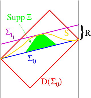
Figure 1: An illustration of the proof that $\Xi$ is smooth. The shaded region is $\mathrm{supp}\ \Xi$, which is compactly contained in $J^{-}(S)$.

Consider now

$$\sigma(t):=\sigma\left(\Xi(\cdot,t),\Phi_{t}-\Psi(\cdot,t)\right)=\sigma\left(\Xi(\cdot,t),\Phi_{t}\right)-\sigma\left(\Xi(\cdot,t),\Psi(\cdot,t)\right)$$ (4.1)

By construction, $\sigma(t_{1})\neq 0$, whereas $\sigma(0)=0$ because $\Phi_{0}=\Psi(\cdot,0)$. A contradiction will now be established by showing that the derivative of $\sigma$ is zero. Since $\Xi$ and $\Psi$ are both smooth solutions of the Klein-Gordon in $D(\Sigma_{0}),$ one of which has compact support, the derivative of the second term of $\sigma(t)$ automatically vanishes. On the other hand, $\Xi(\cdot,t)\in\mathcal{H_{A}}$ for each $t\in[0,t_{1}]$ because it is smooth and of compact support. Further, this one parameter family of vectors is also strongly differentiable in the Hilbert space sense, with derivative $-h\Xi(\cdot,t)$ [8]. By the generalized Stone’s Theorem [6, Theorem 13.35], $\Phi_{0}\in\mathrm{Dom}\ h^{SA}\Leftrightarrow\Phi_{t}\in\mathrm{Dom}\ h^{SA}$, $\Phi_{t}$ is strongly differentiable, and $\Phi_{t}^{\prime}=-h^{SA}\Phi_{t}$. Hence the derivative of the first term of $\sigma(t)$ is $\sigma(-h\Xi(\cdot,t),\Phi_{t})+\sigma(\Xi(\cdot,t),-h^{SA}\Phi_{t})$. Let $\{F_{n}\}\subseteq C_{0}^{\infty}(\Sigma)\oplus C_{0}^{\infty}(\Sigma)$, be a sequence which converges to $\Phi_{t}$ in $\mathcal{H_{A}}$ such that $-h^{SA}F_{n}\rightarrow-h^{SA}\Phi_{t}$. Such a sequence exists because $h^{SA}$ is a closed operator. Since $\mathcal{A}$ is symmetric on smooth data of compact support, and $\mathcal{A}$-norm bounds $L^{2}(d\gamma)\oplus L^{2}(d\gamma)$-norm, it follows that

$$\sigma(-h\Xi(\cdot,t),\Phi_{t})+\sigma(\Xi(\cdot,t),-h^{SA}\Phi_{t}) = \lim_{n\rightarrow\infty}\sigma(-h\Xi(\cdot,t),F_{n})+\sigma(\Xi(\cdot,t),-h^{SA}F_{n})$$

$$= \lim_{n\rightarrow\infty}\left<-h\Xi(\cdot,t)\left.\vphantom{-h\Xi(\cdot,t)}\vphantom{jF_{n}}\right|jF_{n}\right>_{L^{2}\oplus L^{2}}+\left<\Xi(\cdot,t)\left.\vphantom{\Xi(\cdot,t)}\vphantom{j(-h)F_{n}}\right|j(-h)F_{n}\right>_{L^{2}\oplus L^{2}}$$

$$= \lim_{n\rightarrow\infty}\left<j\mathcal{A}\Xi(\cdot,t)\left.\vphantom{j\mathcal{A}\Xi(\cdot,t)}\vphantom{jF_{n}}\right|jF_{n}\right>_{L^{2}\oplus L^{2}}+\left<\Xi(\cdot,t)\left.\vphantom{\Xi(\cdot,t)}\vphantom{j^{2}\mathcal{A}F_{n}}\right|j^{2}\mathcal{A}F_{n}\right>_{L^{2}\oplus L^{2}}$$

$$= \lim_{n\rightarrow\infty}\left<\mathcal{A}\Xi(\cdot,t)\left.\vphantom{\mathcal{A}\Xi(\cdot,t)}\vphantom{F_{n}}\right|F_{n}\right>_{L^{2}\oplus L^{2}}-\left<\Xi(\cdot,t)\left.\vphantom{\Xi(\cdot,t)}\vphantom{\mathcal{A}F_{n}}\right|\mathcal{A}F_{n}\right>_{L^{2}\oplus L^{2}}$$

$$= 0,$$

where $L^{2}$ denotes $L^{2}(d\gamma).$ This establishes the contradiction, so $\Phi_{t}$ and $\Psi(\cdot,t)$ agree a. e. in $D(\Sigma_{0})$. $\blacksquare$

While the proof of the next proposition is conceptually similar to the corresponding result in [3], it differs significantly in detail. The use of the Hilbert space $L^{2}\left(\alpha^{-1}d\gamma\right)$ in [3] allowed a natural identification of the solution (1.3) with a distribution in $H^{0}_{\mathrm{{loc}}}$, and then the strong ellipticity of the operator $A$ was used to show the regularity of $\phi_{t}$. The key to the proof below is the identification of the distribution $X$ (defined below) as a distribution in the negative order Sobolev space $H^{-1}_{\mathrm{{loc}}}\oplus H^{0}_{\mathrm{{loc}}}$. Further, rather than utilizing the ellipticity of the operator $\mathcal{A}h$ directly, its detailed form is used to identify an elliptic operator acting on a piece with sufficient a priori regularity to allow iteration.

Proposition 4.2

Let $\Phi_{t}=:\left(\varphi_{t},\pi_{t}\right)$ be the one-parameter family of vectors (3.5) corresponding to $\Phi_{0}$, and assume 3 holds. If $\Phi_{0}\in\mathrm{Dom}\ \left(h^{SA}\right)^{k}\ \forall\>k\in\mathbb{N}$, then $\varphi(\cdot,t):=\varphi_{t}$ and $\pi(\cdot,t):=\pi_{t}$ are smooth functions on $\Sigma_{t}$ for each fixed $t$.

Proof. Suppose $\Phi_{0}\in\mathrm{Dom}\ h^{SA}$. By Stone’s Theorem $\Phi_{t}\in\mathrm{Dom}\ h^{SA}$, which implies that $h^{SA}\Phi_{t}\in H^{1}_{\mathrm{{loc}}}\oplus H^{0}_{\mathrm{{loc}}}.$ Consider the distribution

$$X(F):=-\left<hF\left.\vphantom{hF}\vphantom{\Phi_{t}}\right|\Phi_{t}\right>_{\mathcal{A}}.$$

By the skew-symmetry of $h^{SA}$ in $\mathcal{H_{A}}$, $X(F)=\int d\gamma F^{T}\mathcal{A}h\Phi_{t}$, where $T$ denotes matrix transpose and $\mathcal{A}$ and $h$ are now viewed as a differential operator on distributions. Hence, $X$, $\varphi_{t}$, and $\pi_{t}$ satisfy the distributional differential equation

$$X=\mathcal{A}h\Phi_{t}=\left[\begin{array}[]{c}\left(\alpha^{2}\gamma^{ab}+\beta^{a}\beta^{b}\right)D_{a}D_{b}\pi_{t}+(D_{a}\beta^{a})D^{b}D_{b}\varphi_{t}+\textrm{lower-order terms}\\ \left(\alpha^{2}\gamma^{ab}+\beta^{a}\beta^{b}\right)D_{a}D_{b}\varphi_{t}+\textrm{lower-order terms}\\ \end{array}\right].$$ (4.2)

Since $\varphi_{t}\in H^{1}_{\mathrm{{loc}}}$ a priori, the second term in the top component of the right hand side of (4.2) is in $H^{-1}_{\mathrm{{loc}}}.$ The lower-order terms on the right hand side are also contained in $H^{-1}_{\mathrm{{loc}}}$. On the other hand, the top left component of $\mathcal{A}$ contains two derivatives and the top right component only one, so $h^{SA}\Phi_{t}\in H^{1}_{\mathrm{{loc}}}\oplus H^{0}_{\mathrm{{loc}}}$ implies that the top component of $X$ is in $H^{-1}_{\mathrm{{loc}}}.$ Hence,

$$E\pi_{t}:=(\alpha^{2}\gamma^{ab}+\beta^{a}\beta^{b})D_{a}D_{b}\pi_{t}\in H^{-1}_{\mathrm{{loc}}}.$$ (4.3)

As $E$ is clearly an elliptic second-order differential operator, $(\ref{smoothb})\Rightarrow\pi_{t}\in H^{1}_{\mathrm{{loc}}}$. With both $\pi_{t}$ and $\varphi_{t}$ established as being in $H^{1}_{\mathrm{{loc}}}$, the lower-order terms in the bottom component of the right hand side of Equation (4.2) are at least $H^{0}_{\mathrm{{loc}}}$. Since the bottom left component of $\mathcal{A}$ contains one derivative and the bottom right component none, $h^{SA}\Phi_{t}\in H^{1}_{\mathrm{{loc}}}\oplus H^{0}_{\mathrm{{loc}}}$ implies that the bottom component of $X$ is in $H^{0}_{\mathrm{{loc}}},$ and hence $E\varphi_{t}\in H^{0}_{\mathrm{{loc}}}\Rightarrow\varphi_{t}\in H^{2}_{\mathrm{{loc}}}.$ Suppose now that $\Phi_{0}\in\mathrm{Dom}\ \left(h^{SA}\right)^{k}$. It is clear that the above argument could be repeated, peeling one $h^{SA}$ at a time. Hence $\varphi_{t}\in H^{k+1}_{\mathrm{{loc}}}$ and $\pi_{t}\in H^{k}_{\mathrm{{loc}}}$. As this is true $\forall\>k$ by assumption, both $\varphi_{t}$ and $\pi_{t}$ are smooth. $\blacksquare$

Proof of Theorem 4.1. It remains only to show that $\varphi$ is smooth solution of the Klein-Gordon equation in $M$. Let $p\in M$, and let $\Sigma_{t_{p}}$ be the slice passing through $p$. Let $\tilde{\Phi}_{t}=e^{h^{SA}(t-t_{p})}\Phi_{t_{p}}$, and let $\tilde{\Psi}$ be the maximal Cauchy evolution of $\Phi_{t_{p}}$ in $D(\Sigma_{t_{p}})$. Again by Proposition 4.1, $\tilde{\Phi}_{t}=\tilde{\Psi}(\cdot,t)$ in $D(\Sigma_{t_{p}})$, which certainly includes some neighborhood of $p$. The definition of $\tilde{\Psi}$ therefore shows that $\varphi$ is smooth and obeys the Klein-Gordon equation in some neighborhood of $p$. As $p$ is arbitrary, the result follows. $\blacksquare$

Theorem 4.2

Under the conditions of Theorem 4.1, $h$ possesses a skew-adjoint extension which has a bounded inverse and conserves the natural symplectic form $\sigma$.

Proof. Because the symplectic form $\sigma$ is continuous with respect to $\mathcal{A}$-norm, the Riesz lemma shows $\exists$ a bounded skew-adjoint operator $T:\mathcal{H_{A}}\rightarrow\mathcal{H_{A}}$ such that $\sigma(\Phi,\Psi)=\left<\Phi\left.\vphantom{\Phi}\vphantom{T\Psi}\right|T\Psi\right>_{\mathcal{A}}\>\forall~{}\Phi,\Psi\in\mathcal{H_{A}}$. Further, $\forall\>F,G\in C_{0}^{\infty}(\Sigma)\oplus C_{0}^{\infty}(\Sigma)$,

$$\left<F\left.\vphantom{F}\vphantom{ThG}\right|ThG\right>_{\mathcal{A}}=\sigma(F,hG)=\left<F\left.\vphantom{F}\vphantom{jhG}\right|jhG\right>_{L^{2}(d\gamma)\oplus L^{2}(d\gamma)}=\left<F\left.\vphantom{F}\vphantom{-j^{2}AG}\right|-j^{2}AG\right>_{L^{2}(d\gamma)\oplus L^{2}(d\gamma)}=\left<F\left.\vphantom{F}\vphantom{G}\right|G\right>_{\mathcal{A}},$$

or that $Th=1$ on $C_{0}^{\infty}(\Sigma)\oplus C_{0}^{\infty}(\Sigma)$. This calculation also shows that $\mathrm{Ran}~{}T$ is dense. Because $T$ is skew-adjoint, this suffices to show that $T^{-1}$ exists and is skew-adjoint [6, Theorem 13.11(b)]. But $T^{-1}|_{C_{0}^{\infty}(\Sigma)\oplus C_{0}^{\infty}(\Sigma)}=h$, so that $T^{-1}$ is a skew-adjoint extension of $h.$ $T$ is by construction bounded, and clearly the symplectic form is conserved by the time evolution associated to $T^{-1}$ because $[T,T^{-1}]=0$. $\blacksquare$

5 Static Spacetimes

It is interesting to compare the first-order formalism in the static slicing with the previously studied second-order formalism [3, 7, 12, 13]. From this analysis will come the result that the definition of the Hilbert space determines the dynamics in these spacetimes. This suggests that the choice of Hilbert space in a general stationary spacetime plays at least as large a role, if not a larger role, in determining the dynamics as does the choice of skew-adjoint extension $h$.

In the static slicing, $\beta^{a}=0$ so $\mathcal{A}$ and $h$ take the form

$$\mathcal{A}=\left[\begin{array}[]{cc}\alpha^{-1}A&0\\ 0&\alpha\end{array}\right]~{}~{}~{}~{}~{}~{}~{}h=\left[\begin{array}[]{cc}0&-\alpha\\ \alpha^{-1}A&0\end{array}\right],$$ (5.1)

where $A$ is the operator (1.2). Thus, $\mathcal{H_{A}}$ decomposes as a direct sum $\mathcal{H_{A}}=\mathcal{X}\oplus\mathcal{Y}$, where $\mathcal{X}=H^{1}_{0}(\alpha d\gamma)$ and $\mathcal{Y}=L^{2}(\alpha d\gamma)$. Another space which plays a role in the analysis is $\mathcal{Z}:=L^{2}(\alpha^{-1}d\gamma)$; this is the Hilbert space in which $A$ is a symmetric operator. Note that $\pi\rightarrow\alpha\pi$ maps $\mathcal{Y}$ bijectively onto $\mathcal{Z}$. This is merely a restatement of the fact the canonical momentum is $\pi=n^{a}\nabla_{a}\varphi$, whereas the time derivative of $\varphi$ is $\frac{\partial\varphi}{\partial t}=\alpha n^{a}\nabla_{a}\varphi=\alpha\pi$.

The relationship between $\mathcal{X}$ and $\mathcal{Z}$ is slightly more complicated. $\mathcal{X}$ is the completion of $C_{0}^{\infty}$ in the norm $\|f\|_{\mathcal{X}}^{2}=\left<f\left.\vphantom{f}\vphantom{Af}\right|Af\right>_{\mathcal{Z}}$. Clearly $\|f\|_{\mathcal{X}}^{2}\leq\|f\|_{A^{\frac{1}{2}}}:=\left<f\left.\vphantom{f}\vphantom{Af}\right|Af\right>_{\mathcal{Z}}+\|f\|_{\mathcal{Z}}^{2}$. However, if 3 holds so that $\alpha\geq\epsilon>0$, then it is also true $(1+\epsilon^{-2})^{-1}\|f\|_{A^{\frac{1}{2}}}\leq\|f\|_{\mathcal{X}}.$ Hence $\mathcal{X}$-norm and $A^{\frac{1}{2}}$-norm are equivalent. The completion of $C_{0}^{\infty}$ in $A^{\frac{1}{2}}$-norm is $q_{F}$, the form-domain of the Friedrichs extension of $A$ [4]. $q_{F}$ is also equal to $\mathrm{Dom}\ A_{F}^{\frac{1}{2}}$, where $A_{F}$ denotes the Friedrichs extension of $A$ [5]. These relationships between $\mathcal{X}$, $\mathcal{Y}$, and $\mathcal{Z}$ are the key understanding the dynamics in static spacetimes.

Theorem 5.1

Let $(M,g_{ab})$ be a static spacetime obeying 3 in the static slicing. If 3 holds, then $h$ is essentially skew-adjoint.

Proof. The deficiency indices of $ih^{\mathbb{C}}$ are computed directly and shown to be zero. Suppose, to the contrary, that $0\neq\Phi=(\varphi,\pi)\in K_{\pm}$. This means that $\forall\>F=(f,g)\in C_{0}^{\infty}(\Sigma)\oplus C_{0}^{\infty}(\Sigma),$ $\Phi$ satisfies $\int d\gamma\Phi^{T}\mathcal{A}(ih^{\mathbb{C}}\pm i)F=0$. The preceding discussion shows that the map $(\varphi,\pi)\rightarrow(\varphi,\alpha\pi)$ injects $\mathcal{H_{A}}\hookrightarrow\mathcal{Z}\oplus\mathcal{Z}$, so that the index equations can be written as

$$-\left<\varphi\left.\vphantom{\varphi}\vphantom{Ag}\right|Ag\right>_{\mathcal{Z}}\mp\left<\alpha\pi\left.\vphantom{\alpha\pi}\vphantom{g}\right|g\right>_{\mathcal{Z}} = 0$$ (5.2)

$$\left<\alpha\pi\left.\vphantom{\alpha\pi}\vphantom{Af}\right|Af\right>_{\mathcal{Z}}\mp\left<\varphi\left.\vphantom{\varphi}\vphantom{Af}\right|Af\right>_{\mathcal{Z}} = 0.$$ (5.3)

Equation (5.2) is nothing but the statement $\varphi\in\mathrm{Dom}\ A^{*}$ (where the adjoint is taken in $\mathcal{Z}$) and $A^{*}\varphi=\mp\alpha\pi$. Equation (5.3) then becomes $A^{*}(\alpha\pi)=\pm A^{*}\varphi.$ Clearly, one solution is $\alpha\pi=\varphi$, or $A^{*}\varphi=-\varphi$. Suppose that $\alpha\pi=\varphi+\delta$ were a second solution. This would mean that $A^{*}\delta=0$, or that $\left<F\left.\vphantom{F}\vphantom{(\delta,0)}\right|(\delta,0)\right>_{\mathcal{A}}=0\>\forall\>F\in C_{0}^{\infty}(\Sigma)\oplus C_{0}^{\infty}(\Sigma).$ As $C_{0}^{\infty}(\Sigma)\oplus C_{0}^{\infty}(\Sigma)$ is dense in $\mathcal{H_{A}}$, it follows that $(\delta,0)=0$ in $\mathcal{H_{A}}.$ Thus $A^{*}\varphi=-\varphi,~{}\alpha\pi=\varphi$ is the unique solution to (5.2), (5.3). Now, let $F_{n}:=\{(f_{n},g_{n})\}\subseteq C_{0}^{\infty}(\Sigma)\oplus C_{0}^{\infty}(\Sigma)$ be a sequence which converges to $\Phi$ in $\mathcal{H_{A}}$. Since $\|F_{n}\|_{\mathcal{A}}\geq\|F_{n}\|_{\mathcal{Z}\oplus\mathcal{Z}}$, it follows that $f_{n}\rightarrow\varphi$ in $\mathcal{Z}$. But $\mathcal{X}=q_{F}$, which means that $\|(f_{n},0)\|_{\mathcal{A}}\rightarrow\left<\varphi\left.\vphantom{\varphi}\vphantom{A\varphi}\right|A\varphi\right>_{\mathcal{Z}}=-\|\varphi\|_{\mathcal{Z}}^{2}$, which is clearly impossible. Hence $K_{\pm}=\{0\}$ and $h$ is essentially skew-adjoint. $\blacksquare$

In [7] it was shown that any reasonable prescription agrees with the second-order formalism on $C_{0}^{\infty}$ data for some choice of positive, self-adjoint extension $A_{E}$ of $A$. The following theorem shows, without invoking the result of [7], that the first-order formalism agrees with the second order formalism when the Friedrichs extension is chosen. It actually shows a stronger result, namely that the prescriptions agree for data in $\mathcal{H_{A}}.$

Theorem 5.2

Let $(M,g_{ab})$ be a static spacetime obeying 3, and suppose that 3 holds. In the static slicing define $U^{(1)}:\mathcal{H_{A}}\rightarrow\mathcal{H_{A}}$ by $U^{(1)}=e^{-\bar{h}t}$, where $\bar{h}$ denotes the operator closure of $h$ in $\mathcal{H_{A}}$, and let $U^{(2)}:\mathcal{Z}\oplus\mathcal{Y}\rightarrow\mathcal{Z}\oplus\mathcal{Y}$ be given by

$$U^{(2)}(t)=\left[\begin{array}[]{cc}\cos\left(A_{F}^{\frac{1}{2}}t\right)&A_{F}^{-\frac{1}{2}}\sin\left(A_{F}^{\frac{1}{2}}t\right)\alpha\\ -\alpha^{-1}A_{F}^{\frac{1}{2}}\sin\left(A_{F}^{\frac{1}{2}}t\right)&\alpha^{-1}\cos\left(A_{F}^{\frac{1}{2}}t\right)\alpha\\ \end{array}\right],$$

where $A_{F}$ is the Friedrichs extension of $A$ in $\mathcal{Z}$. Then $U^{(2)}(-t)U^{(1)}(t)$ is a well-defined map $\mathcal{H_{A}}\rightarrow\mathcal{H_{A}}$, and further

$$U^{(2)}(-t)U^{(1)}(t)=\mathbb{I}_{2\times 2}.$$ (5.4)

Proof. Notice that the operators in (5.4) correspond to evolving the initial state by a time $t$ in the first-order formalism, then evolving time backward by $t$ in the second-order formalism. Thus, if $U^{(2)}(-t)U^{(1)}(t)$ maps $\mathcal{H_{A}}$ to itself and further $U^{(2)}(-t)U^{(1)}(t)=\mathbb{I}_{2\times 2}$, then these two evolutions invert each other, and hence the first-order and second-order formalism agree.

Let $(\varphi_{0},\pi_{0})\in\mathcal{H_{A}}$ and define

$$\Upsilon_{t}:=U^{(2)}(-t)U^{(1)}(t)(\varphi_{0},\pi_{0}).$$

It will at first be assumed that $(\varphi_{0},\pi_{0})\in\mathrm{Dom}\ \bar{h}$. This assumption will be used to show that $\Upsilon_{t}$ differentiable in $\mathcal{Z}\oplus\mathcal{Y}$ and, in fact, constant. It will then be shown that $\Upsilon_{t}$ is constant for arbitrary $(\varphi_{0},\pi_{0})\in\mathcal{H_{A}}$, which establishes the result (5.4).

It is first necessary to show that $U^{(2)}(-t)U^{(1)}(t)$ maps $\mathcal{H_{A}}\rightarrow\mathcal{H_{A}}$ so that $\Upsilon_{t}$ is well-defined. Because Theorem 5.1 shows that $h$ is essentially skew-adjoint, its closure $\bar{h}$ is skew-adjoint. This suffices to show that $U^{(1)}(\varphi_{0},\pi_{0})$ is a well-defined vector in $\mathcal{H_{A}}$. As noted above, $\mathcal{X}=q_{F}=\mathrm{Dom}\ A_{F}^{\frac{1}{2}}$. Hence the $\mathcal{X}$ component of $\Upsilon_{t}$ is well-defined because (i) $\cos(A_{F}^{\frac{1}{2}}t)$ is a bounded operator (on $\mathcal{Z}$) which leaves $q_{F}$ invariant, and (ii) $A^{-\frac{1}{2}}_{F}\sin(A_{F}^{\frac{1}{2}}t)$ is a bounded operator on $\mathcal{Z}$ with range contained in $\mathrm{Dom}\ A_{F}^{\frac{1}{2}}$, and $\alpha$ maps $\mathcal{Y}$ to $\mathcal{Z}$. On the other hand, the $\mathcal{Y}$ component of $\Upsilon_{t}$ is well-defined because (iii) $\psi\in\mathcal{X}\Leftrightarrow\alpha^{-1}A_{F}^{\frac{1}{2}}\sin(A_{F}^{\frac{1}{2}}t)\psi\in\mathcal{Y}$, and (iv) $\cos(A_{F}^{\frac{1}{2}}t)$ is a bounded operator on $\mathcal{Z}$, combined with the fact that $\alpha$ maps $\mathcal{Y}$ to $\mathcal{Z}$ bijectively. Notice that (iii) and (iv) would continue to hold if $A_{F}$ were replaced by $A_{E}$ in the definition of $U^{(2)}(t)$. However, (i) would fail for an arbitrary extension. Further, (ii) necessarily fails for any other extension $A_{E}$ because $q_{F}$ is the closure of the quadratic form associated to $A$ [4]. This implies that $\mathrm{Dom}\ A_{E}^{\frac{1}{2}}\supsetneq\mathrm{Dom}\ A_{F}^{\frac{1}{2}}$ [5], and and hence $A_{E}^{-\frac{1}{2}}\sin(A_{E}^{\frac{1}{2}}\alpha)$ maps $\mathcal{Y}$ outside of $\mathcal{X}$. Therefore this theorem identifies $A_{F}$ as the unique self-adjoint extension whose dynamics agree with the first-order formalism.

Suppose now that $(\varphi_{0},\pi_{0})\in\mathrm{Dom}\ \bar{h},$ which by definition is the closure of $C_{0}^{\infty}(\Sigma)\oplus C_{0}^{\infty}(\Sigma)$ in the norm:

$$\|(f,g)\|_{\bar{h}}^{2} := \|(f,g)\|_{\mathcal{A}}^{2}+\|h(f,g)\|_{\mathcal{A}}^{2}$$

$$= \left<f\left.\vphantom{f}\vphantom{Af}\right|Af\right>_{\mathcal{Z}}+\left<f\left.\vphantom{f}\vphantom{A^{2}f}\right|A^{2}f\right>_{\mathcal{Z}}+\|\alpha g\|_{\mathcal{Z}}^{2}+\left<\alpha g\left.\vphantom{\alpha g}\vphantom{A\alpha g}\right|A\alpha g\right>_{\mathcal{Z}}.$$ (5.5)

On the one hand, $\frac{\epsilon^{2}}{m^{2}}\left<f\left.\vphantom{f}\vphantom{f}\right|f\right>\leq\left<f\left.\vphantom{f}\vphantom{Af}\right|Af\right>$. On the other hand, the Cauchy-Schwartz inequality and the fact that $A$ is symmetric imply that

$$\left<f\left.\vphantom{f}\vphantom{Af}\right|Af\right>_{\mathcal{Z}}\leq\left\|f\right\|_{\mathcal{Z}}\left\|Af\right\|_{\mathcal{Z}}\leq\frac{1}{2}\left(\left<f\left.\vphantom{f}\vphantom{f}\right|f\right>_{\mathcal{Z}}+\left<Af\left.\vphantom{Af}\vphantom{Af}\right|Af\right>_{\mathcal{Z}}\right)=\frac{1}{2}\left(\left<f\left.\vphantom{f}\vphantom{f}\right|f\right>_{\mathcal{Z}}+\left<f\left.\vphantom{f}\vphantom{A^{2}f}\right|A^{2}f\right>_{\mathcal{Z}}\right).$$

Thus, the first two terms in (5.5) are norm equivalent to $\left<f\left.\vphantom{f}\vphantom{f}\right|f\right>_{\mathcal{Z}}+\left<f\left.\vphantom{f}\vphantom{A^{2}f}\right|A^{2}f\right>_{\mathcal{Z}},$ which means that $\varphi_{0}\in\mathrm{Dom}\ \bar{A}\subseteq\mathrm{Dom}\ A_{F}$. The last two terms in (5.5) are operator-closure norm for $A_{F}^{\frac{1}{2}}$, so $\alpha\pi_{0}\in\mathrm{Dom}\ A_{F}^{\frac{1}{2}}.$

Let $\Psi=(\psi,\theta)$ be such that $\psi\in\mathrm{Dom}\ A_{F}$ and $\theta\in\mathcal{Y}.$ Arguments similar to those which prove Stone’s Theorem as well as the fact that $\alpha$ maps $\mathcal{Y}$ to $\mathcal{Z}$ bijectively show that $U^{(2)}(t)\Psi$ is strongly differentiable in $\mathcal{Z}\oplus\mathcal{Y}$ with derivative

$$D^{(2)}U^{(2)}\Psi:=\left[\begin{array}[]{cc}0&\alpha\\ -A_{F}&0\end{array}\right]U^{(2)}\Psi.$$

By the generalized Stone’s theorem [6, Theorem 13.35], the strong derivative of $U^{(1)}(t)(\varphi_{0},\pi_{0})$ exists in $\mathcal{H_{A}}$ and is given by

$$D^{(1)}U^{(1)}(t)(\varphi_{0},\pi_{0}):=-\bar{h}(\varphi_{t},\pi_{t})=(-\alpha\pi_{t},\bar{A}\varphi_{t}).$$

The last equality follows because action of $h$ on $f$ agrees with the action of $A$ on $f$ in a core domain $C_{0}^{\infty}$. However, $\mathcal{H_{A}}$-norm bounds $\mathcal{Z}\oplus\mathcal{Y}$-norm, so any one parameter family of vectors which is norm differentiable in $\mathcal{H_{A}}$ is also norm differentiable in $\mathcal{Z}\oplus\mathcal{Y}$. Hence $U^{(1)}(t)(\varphi_{0},\pi_{0})$ is strongly differentiable in $\mathcal{Z}\oplus\mathcal{Y}.$ The generalized Stone’s theorem further shows that $U^{(1)}(t)(\varphi_{0},\pi_{0})\in\mathrm{Dom}\ \bar{h}$ and hence that $U^{(1)}(t)(\varphi_{0},\pi_{0})\in\mathrm{Dom}\ \bar{A}\oplus\mathcal{Y}$ for all $t\in\mathbb{R}$. Thus, the Leibnitz rule may be used, yielding

$$\Upsilon_{t}^{\prime}=U^{(2)}(-t)\left[D^{(1)}-D^{(2)}\right]U^{(1)}(t)\left(\begin{array}[]{c}\varphi_{0}\\ \pi_{0}\end{array}\right),$$

Again because the $\mathcal{X}$ component of $\mathrm{Dom}\ \bar{h}$ is $\mathrm{Dom}\ \bar{A}\subseteq\mathrm{Dom}\ A_{F}$, it follows that $D^{(2)}|_{\mathrm{Dom}\ \bar{h}}=D^{(1)}$, or $\Upsilon^{\prime}_{t}=0.$ Hence $\Upsilon_{t}$ is a constant equal to $\Upsilon_{0}=(\varphi_{0},\pi_{0}).$

It remains only to show that $\Upsilon_{t}=\Upsilon_{0}$ for arbitrary $(\varphi_{0},\pi_{0})\in\mathcal{H}_{A}.$ However, $U^{(1)}(t)$ is a unitary transformation by the spectral theorem. $U^{(2)}(-t)$ is a bounded operator on $\mathcal{H_{A}}$, as can be shown by a straightforward computation utilizing facts (i)-(iv). Since it inverts the unitary operator $U^{(1)}(t)$ on the dense domain $\mathrm{Dom}\ \bar{h}$, $U^{(2)}(-t)|_{\mathcal{H_{A}}}$ is also unitary and $\left(U^{(2)}(-t)|_{\mathcal{H_{A}}}\right)^{-1}=U^{(1)}(t)$. Thus, $U^{(2)}(-t)U^{(1)}(t)=\mathbb{I}_{2\times 2}$ on $\mathcal{H_{A}}$. $\blacksquare$

Theorem 5.1 suggests that the first-order prescription is unique. However, it is known [12, 13] that $A$ is not essentially self-adjoint in $\mathcal{Z}$—and hence the choice of dynamics is not unique—in a variety of static spacetimes. This raises the question of why the first-order formalism appears unique, but the proof of Theorem 5.2 has already provided the answer. It appears unique because $\mathcal{H_{A}}$ was defined as the completion of $C_{0}^{\infty}(\Sigma)\oplus C_{0}^{\infty}(\Sigma)$ in $\mathcal{A}$ norm. To produce other dynamics, define $\tilde{}\mathcal{H}_{\mathcal{A}}:=q_{E}\oplus\mathcal{Y}$, where $q_{E}$ is the form domain of any other positive, self-adjoint extension $A_{E}$ of $A$ in $\mathcal{Z}$. Since $C_{0}^{\infty}(\Sigma)\oplus C_{0}^{\infty}(\Sigma)$ is no longer dense in $\mathcal{H_{A}}$, one cannot define $h$ on this domain and take its closure. However, $\tilde{h}$ may be defined directly in terms of the spectral resolution of $A_{E}$. The obvious modification of the proof of Theorem 5.2 then shows that the dynamics defined by $\tilde{h}$ agrees with the dynamics defined by $A_{E}$ on data contained in $q_{E}\oplus\mathcal{Y}$. Thus, in the first-order formalism, it is the choice of Hilbert space that encodes the “boundary conditions at the singularity”, as opposed to the second-order formalism where they are encoded in the choice of self-adjoint extension of $A$.

It should be emphasized, as noted above, that care must be taken to ensure that an operator defined on an energy-type Hilbert space is in fact densely defined. It appears that this point was overlooked in the analysis of [13], leading to a mistaken conclusion that the operator $A$ of that reference is not essentially self-adjoint in certain spherically symmetric spacetimes. In [13], the operator (1.2), initially defined on $C_{0}^{\infty}(\Sigma)$, was viewed as an operator in $H^{1}$. However, if $C_{0}^{\infty}$ is not a dense subspace of $H^{1}$, then $A$ is not well-defined. On the other hand, if $C_{0}^{\infty}$ is dense, then the deficiency subspaces of $A$ are trivial because the solutions to $(A^{*}\pm i)\phi=0$, while they are square integrable, are not well-approximated by $C_{0}^{\infty}$ functions. This correction actually strengthens the conclusion of that work, in that it means that all the spacetimes considered there are “wave regular,” that is, possessing an essentially self-adjoint $A$. This suggests that the essential skew-adjointness of $h$ in static spacetimes may be a general property of using Sobolev (energy) Hilbert spaces and not of the first-order formalism per se.

6 Field Quantization

There is a general prescription for defining a quantum vacuum associated to any give notion of energy which was originally proposed by Ashtekar and Magnon [14], further developed by Kay [8], and generalized by Chmielowski [15]. For a globally hyperbolic spacetime, the procedure is as follows. Let $\Sigma$ be a Cauchy surface for the globally hyperbolic spacetime $(M,g_{ab})$ . Denote by $(S,\sigma)$ the space of classical solutions, which may be identified with the initial data $C_{0}^{\infty}(\Sigma)\oplus C_{0}^{\infty}(\Sigma)$, together with the symplectic form, which may be done as the initial value problem is well-posed in these spacestimes. Let $\mu$ be any inner product on $S$ which satisfies the inequality

$$\left|\sigma(\Phi,\Psi)\right|\leq 2\sqrt{\mu(\Psi,\Psi)\mu(\Phi,\Phi)},$$ (6.1)

and let $\mathcal{H}_{\mu}$ denote the completion of $S$ in $\mu$-norm. Kay and Wald [16] showed that $\mu$ defines a state in the class of quasifree states, which includes both vacuum and thermal states. ($\frac{1}{2}\mu$ is essentially the real part of the two-point function of the state. See [16] or [15] for the details.) As $\sigma$ is skew-symmetric and bounded on $\mathcal{H}_{\mu}$, there is a unique, bounded, skew-adjoint operator $T_{\mu}$ on $\mathcal{H}_{\mu}$ such that

$$\sigma(\Phi,\Psi)=2\mu(\Phi,T_{\mu}\Psi)\>\forall\>\Phi,\Psi\in S.$$ (6.2)

Define a new inner product on $S$ by $\tilde{\mu}(\Phi,\Psi)=\mu(\Phi,|T_{\mu}|\Psi),$ where $|T_{\mu}|$ denotes the “absolute value” of $T_{\mu}$ (see, e.g., [5]). The state defined by $\tilde{\mu}$ is pure in addition to being quasifree, and hence is a vacuum state [15]. Chmielowski further showed that if $\mu$ is the Hamiltonian (3.1) (rescaled so that it saturates the inequality (6.1)), then the vacuum state so defined is the well-known “frequency-splitting” ground state associated to a timelike Killing field.

The assumption of global hyperbolicity was used subtly in the above argument, allowing the identification of $C_{0}^{\infty}(\Sigma)\oplus C_{0}^{\infty}(\Sigma)$ with the space of solutions. This meant that the symplectic form defined via the integral (3.6) was well-defined on the space of solutions $S$ because it is non-degenerate and conserved for solutions of the wave equation. Similarly, the norm $\mu$ on the space of solutions could be defined via an integral on some spatial slice because there was a natural identification of solutions with initial data on that slice. In the non-globally-hyperbolic case, the situtation is much more complicated. In the absence of any prescription for selecting solutions, a given initial datum might be identified with many different solutions of the equation. Hence, the Hamiltonian (3.1) would fail to define an inner product because there would be non-zero solutions which have zero norm. Worse yet, the sympletic form (3.6) would fail to be non-degenerate. Thus, the quantum vacuum cannot be defined because the space of all solutions to the wave equation is “too large.” By analogy with the globally hyperbolic space, one might try to define a smaller space $\tilde{S}$ by requiring that the solutions be compactly supported on all spatial slices. However, the time evolution carries $C_{0}^{\infty}(\Sigma)\oplus C_{0}^{\infty}(\Sigma)$ data to non-compactly supported data, in general, and thus $C_{0}^{\infty}(\Sigma)\oplus C_{0}^{\infty}(\Sigma)$ is “too small” as the initial data set.

However, the prescription for defining dynamics presented above is automatically defined not on just $C_{0}^{\infty}(\Sigma)\oplus C_{0}^{\infty}(\Sigma)$ but on the whole Hilbert space $\mathcal{H_{A}}$. Further, $\sigma$ extends to a bounded bilinear form on $\mathcal{H_{A}}$, so that $\mathcal{H_{A}}$ is a “small enough” space to have a well-defined symplectic structure. If one uses the extension $h^{SA}=T^{-1}$ (where $T$ is as in the proof of Theorem 4.2), $\sigma$ is conserved for all solutions with initial data in $\mathrm{Dom}~{}h^{SA}$, so that space can be identified with a space of solutions. Since the prescription automatically conserves $\mathcal{A}$-norm, if an inner product $\mu$ is defined by $\mu(\Phi,\Phi)=\left<\Phi\left.\vphantom{\Phi}\vphantom{\Phi}\right|\Phi\right>_{\mathcal{A}}$ (plus appropraite rescaling to satisfy (6.1)), then $\tilde{\mu}=\mu$. This may be seen explicitly from the proof of Theorem 4.2, which shows that $\left|T_{\mu}\right|=\left|T\right|$. The fact that $h^{SA}=T^{-1}$ has a bounded inverse has an important physical consequence: the real part of the two-point function in the quantum vacuum associated to $T^{-1}$ is given by

$$\frac{1}{2}\tilde{\mu}_{T^{-1}}(\Phi,\Psi)=\frac{1}{2}\left<\Phi\left.\vphantom{\Phi}\vphantom{\left|T\right|\Psi}\right|\left|T\right|\Psi\right>_{\mathcal{A}}.$$

However, if $T$ were not bounded, then the smeared two-point function would diverge. Hence, $|T|^{-1}$ has a “mass gap” and thus avoids “infrared divergences” in its quantum vacuum.

The foregoing analysis, along with the results of [12], [13] that in certain static spacetimes the operator $A$ is not essentially self-adjoint, shows there are many different “energy splitting” ground states possible in a non-globally-hyperbolic spacetime. In these static spacetimes, $T$ is a fixed, bounded function of $A_{E}^{-\frac{1}{2}}$, where $A_{E}$ is the self-adjoint extension used to define the Hilbert space $\tilde{}\mathcal{H}_{\mathcal{A}}$. Since different extensions have different spectral decompositions (on $\mathcal{Z}$) and $A_{E}^{-\frac{1}{2}}$ is a bounded operator, it follows that $T$ is different for different choices of $\tilde{}\mathcal{H}_{\mathcal{A}}$, even when restricted to $C_{0}^{\infty}(\Sigma)\oplus C_{0}^{\infty}(\Sigma)$. This contrasts sharply with the globally hyperbolic case, where each timelike Killing field defines a unique ground state, and different timelike Killing fields almost always give rise to the same “frequency-splitting” ground state [15].

7 Conclusions

The present work shows that a dynamical prescription with sensible properties can be given in a large class of stationary spacetimes. In the case of static spacetimes obeying 3, the present prescription agrees with the previously studied second-order prescription for a particular choice of extension, namely $A_{F}.$ The basic prescription can also be modified to include all reasonable dynamics (in the sense of [7]) handled by the second-order formalism. Nonetheless, the present work leaves many questions unanswered.

First and foremost among these is whether the prescriptions given by using the first-order formalism with different slicings in the same spacetime give rise to the same dynamics. While it is easy to construct examples of spacetimes with inequivalent slicings satisfying 3, it is not clear whether the dynamics produced by these slicings agree. It seems sensible that the preferred extension $h^{SA}=T^{-1}$ would give rise to the same solutions in any slicing, but this remains to be shown. A related question is whether $h$ ever has skew-adjoint extensions other than $T^{-1}$. The proof presented above does not preclude this possibility, but no examples have thus far been found, either. A different question is whether $h$ possesses a skew-adjoint extension in an arbitrary stationary spacetime. Assumptions (A) and (B) were used in crucial ways in the proofs in Section 4. However, it is not known whether Theorems 4.1 or 4.2 fail without these assumptions, or whether (A) and (B) are only needed because of the method of proof used. Along these same lines, it would be interesting to compare the first and second-order formalisms in static spacetimes when 3 is dropped. If they could be shown to agree, then the results of Theorem 4.1 would follow from the proof in the second-order formalism, without imposing 3 (and possibly 3). On the other hand, when 3 fails, it is no longer true that $\mathcal{X}$-norm bounds some multiple of $A^{\frac{1}{2}}$-norm. Hence $\mathcal{X}$ may properly contain $q_{F}$, which considerably complicates the analysis of Section 5.

All of these question deal purely with the classical theory, but there are questions regarding the quantum theory as well. The analysis of Section 6 analyzed the linear theory only. In the past few years, a general prescription for defining interacting quantum field theory in globally hyperbolic, curved spacetimes has been given [17, 18, 19, 20]. This prescription relies on detailed properties of the so-called “wavefront set” of the Green’s functions of the free theory. One additional question to be answered is whether the solutions defined by the prescription given in the present work allow the definition of Green’s functions satisfying these same conditions. This would allow an interacting quantum theory to be defined in non-globally-hyperbolic spacetimes in an analogous fashion.

Acknowledgments

The author is greatly indebted to Robert Wald for his constant support and advice. Thanks are also due to Stefan Hollands, Daniel Hoyt, and Mike Seifert for many useful discussions. This work was supported in part by a National Science Foundation Graduate Research Fellowship and NSF Grant PHY00-90138 to the University of Chicago.

References

- [1] R. M. Wald, General Relativity (U. of Chicago P., Chicago, 1984)
- [2] R. Penrose, in General Relativity: An Einstein Centenary Survey, edited by S. W. Hawking and W. Israel (Cambridge U. P., Cambridge, England, 1979).
- [3] R. M. Wald, J. Math. Phys. 21, 2802 (1980).
- [4] M. Reed and B. Simon, Fourier Analysis, Self-Adjointness (Academic, New York, 1975).
- [5] M. Reed and B. Simon, Methods of Modern Mathematical Physics I: Functional Analysis, Revised and Enlarged Ed (Academic, New York, 1980).
- [6] W. Rudin, Functional Analysis, 2nd Ed, (McGraw-Hill, Boston, 1991).
- [7] A. Ishibashi and R. M. Wald, Class. Quant. Grav. 20, 3815 (2003) [arXiv:gr-qc/0305012].
- [8] B. S. Kay, Commun. Math. Phys. 62, 55 (1978).
- [9] J. von Neumann, Math. Ann. 102, 49 (1930).
- [10] M. H. Stone, Amer. Math. Soc. Colloq. Pub., 15, 1932.
- [11] H.-J. Seifert, Gen Rel Grav. 8, 815 (1977)
- [12] G. T. Horowitz and D. Marolf, Phys. Rev. D 52, 5670 (1995) [arXiv:gr-qc/9504028].
- [13] A. Ishibashi and A. Hosoya, Phys. Rev. D 60, 104028 (1999) [arXiv:gr-qc/9907009].
- [14] A. Ashtekar and A. Magnon, Proc. Roy. Soc. Lond. A 346, 375 (1975).
- [15] P. Chmielowski, Class. Quant. Grav. 11, 41 (1994).
- [16] B. S. Kay and R. M. Wald, Horizon,” Phys. Rept. 207, 49 (1991).
- [17] R. Brunetti, K. Fredenhagen and M. Kohler, Commun. Math. Phys. 180, 633 (1996) [arXiv:gr-qc/9510056].
- [18] R. Brunetti and K. Fredenhagen, Commun. Math. Phys. 208, 623 (2000) [arXiv:math-ph/9903028].
- [19] S. Hollands and R. M. Wald, Commun. Math. Phys. 223, 289 (2001) [arXiv:gr-qc/0103074].
- [20] S. Hollands and R. M. Wald, Commun. Math. Phys. 231, 309 (2002) [arXiv:gr-qc/0111108].