WKB metastable quantum states of a de Sitter–Reißner-Nordström dust shell

Abstract

We study the dynamics of a spherically symmetric dust shell separating two spacetime domains, the interior one being a part of the de Sitter spacetime and the exterior one having the extremal Reißner-Nordström geometry. Extending the ideas of previous works on the subject, we show that the it is possible to determine the (metastable) WKB quantum states of this gravitational system.

1 Introduction

The dynamics of relativistic thin shells is a recurrent topic in the literature about the classical theory of gravitating systems and the still ongoing attempts to obtain a coherent description of their quantum behaviour. Certainly, a good reason to make this system a preferred one for a lot of models is the clear, synthetic description of its dynamics in terms of Israel’s junction conditions [1, 2] (the null case, considered in detail in the seminal paper of C. Barrabes and W. Israel [3], is also interesting for null-like surfaces [4], i.e. light-like matter shells [5], for which an Hamiltonian treatment is given in [6] generalizing the approach described in [7]). Using this formalism, which has an intuitive geometric meaning, many relevant aspects of gravitation have been brought into light.

Gravitating shells have indeed been considered as natural models for different astrophysical problems: the description of variable cosmic objects [9] and of specific aspects (like ejection [10] or crossing of layers [11], critical phenomena [12], perturbations [13] and back-reaction [14]) in gravitational collapse [15, 16, 17] are only a few examples.

Moreover, at larger scales, specific configurations of shells have also been considered to construct cosmological models [18] (even with hierarchical (fractal) structure [19]), to analyze phase transitions in the early universe [20] or to describe cosmological voids [21]; semiclassical models have tackled the problem of avoiding the initial singularity of the Big-Bang scenario by quantum tunnelling [22, 23, 24].

As a matter of fact quantum semiclassical models have conveniently been employed as useful simple examples to better understand possible properties and modifications to the spacetime structure at scales at which quantum effects should give significant contributions to gravitational physics. Apart from the quantization of the gravitating shell itself (as in [25, 26]), considered also in the context of gravitational collapse [27], models have been proposed to study quantum properties of black holes [28, 29, 30] and their formation process [31] as well as to analyze wormhole spacetimes [32, 33, 34, 35] and the quantum stabilization of their instability [36, 37], targeting the fuzzy properties of spacetime foam [38] and Planck scale physics [39].

Other problems of fundamental nature in quantum gravity have received attention through the study of shell dynamics: as an exemplificative list, we mention here Hawking radiation [40, 30, 41] the horizon problem in wormhole spacetimes [42], the time problem in canonical relativity [43], the problem of localization of gravitational energy [44], the thermodynamics of self-gravitating systems [45, 46] and the possibility of connecting compact with non-compact dimensions [47].
Many of the above discussions have been performed under the simplifying assumption of spherical symmetry: this is especially useful in the quantum treatment, because the minisuperspace approximation greatly reduces the complexity of the mathematical treatment.
But, at least at the classical level, studies have also been performed for cylindrical models (see e.g. [48, 49, 50]).

With the development of the models shortly cited above, particularly those involved with the quantization of the system, many subtleties emerged as byproducts of corresponding difficulties already encountered in tentative approaches to Quantum Gravity and mainly related to the reparametrization invariance of the theory. Since the junction conditions, essentially, are a first integral of the equations of motion of the shell, many authors revolved their attention to the derivation of these equations starting from an action principle. A consistent Lagrangian/Hamiltonian formalism has been developed [51, 52, 53, 54] (also reduced by spherical symmetry [55]), and the relevant degrees of freedom of the system [56] discussed together with a variational principle, which is also the subject of [57, 58] (interesting considerations can also be found in [59]).

Recently even more interest in the thin shell formalism is coming thanks to the development of brane world scenarios, where our universe is seen as a four dimensional brane embedded in a five dimensional space [60, 61]. This configuration can be given a wormhole interpretation [62] and has also been analyzed from the point of view of energy conditions [63] (not) satisfied in the higher dimensional background.

In these and other studies, different cases of junctions between spacetimes have been considered: for example between anti de Sitter and anti de Sitter [62], Friedmann-Robertson-Walker and Friedmann-Robertson-Walker [34], Minkowski and Minkowski [37, 38], Schwarzschild and Schwarzschild [36, 11, 9, 6], Reißner-Nordström and Reißner-Nordström [15, 33], de Sitter and Reißner-Nordström [63], de Sitter and Schwarzschild [64, 23, 81], de Sitter and Schwarzschild-de Sitter [65], de Sitter and Vaidya [24], Friedmann-like and Reißner-Nordström [66], Minkowski and Friedmann [21], Minkowski and Reißner-Nordström [15, 41, 67], Minkowski and Schwarzschild [28, 31, 25, 14, 43, 29], Minkowski and Vaidya [12], Schwarzschild and Reißner-Nordström [67], Schwarzschild and Schwarzschild-anti de Sitter [47], Schwarzschild and Vaidya [46], Tolman and Friedman [19], Lemaître-Tolman-Bondi and Lemaître-Tolman-Bondi [18].

In this paper we are also going to use a general relativistic shell to analyze, even if only at the semiclassical level, the problem of quantization of a gravitational system. We will restrict ourselves, as it has been done in many of the papers cited above, to the spherically symmetric case and we will study the semiclassical quantum dynamics in the case in which the shell separates an interior spacetime of the de Sitter geometry, from an exterior of the extremal Reißner-Nordström type. An observer crossing the shell will naively see some non-vanishing vacuum energy density to be converted into physical properties like charge and mass. From the classical dynamics there are no restrictions on the values of the physical parameters characterizing the geometry of spacetime. But, starting from a Hamiltonian description of the shell dynamics, we will try to analyze its quantum behaviour. Lacking a full theory of quantum gravity, which would of course be the natural setting for this kind of problem, we will tackle it only at the semiclassical level: under this word, we will understand that the action for the shell is given as an integer multiple of the quantum, $\hbar$. We will see that this condition results in a constraint on the parameters for the interior and exterior geometries. This is hardly surprising: indeed a full quantum theory of gravity, would have the task of determining the probability amplitude for a given configuration of the three-geometries taught as points in superspace; in our quantum minisuperspace approach, the only free parameters remain the constants (de Sitter cosmological horizon, charge and mass) fixing the interior and exterior metrics, and is thus as a relation among them that the semiclassical quantization conditions realizes itself.

With the above ideas in mind the paper is organized as follows.
In section 2 we will set up our model by giving all relevant definitions; we will also recall some well known results adapted to our special case, to fix notations and conventions, and will present all relevant dynamical quantities for the computations that follows. The Bohr–Sommerfeld quantization condition is also recalled. Then, in section 3 the classical dynamics of the system is sketched and the associated spacetime structure discussed, with particular emphasis on the bounded trajectories. This prepares the ground for section 4, where the classical action is numerically evaluated for bounded trajectories. This result is then used in section 5 to show how the Bohr–Sommerfeld quantization condition characterizes the properties of the semiclassical quantum system. After a preliminary rough estimate (subsection 5.1), we present the semi-classical results for the quantum levels of the shell and the corresponding internal/external geometries and approximate the results with a properly chosen analytic (polynomial) expression. Discussion about the results and possible refinements of the model follow in section 6.
Five short appendices are devoted to a more detailed analysis of some technical points. The turning points of the classical motion are discussed in A. The issue about the stability of the classical solution against single particle decay is studied in B. C shows that the bounded trajectories are not affected by change of direction of the normal to the shell trajectory. The characterization of the singularity that appears in the integral for the computation of the classical action as an integrable one is done in D and the determination of the leading terms in the integrand of the same computation is the topic of E.

2 Preliminaries

In this section we define the system, motivate the settings under which we study its classical and semiclassical dynamics and recall some useful results and definitions.

Let us thus start with the geometrodynamical framework, by considering two spacetime domains joined along a spherically symmetric timelike shell. We assume, for the region we shall call the interior, a geometry of the de Sitter type [68, 69, 70] (we denote with $H$ the cosmological horizon), so that the metric in static coordinates is:

$$g_{\mathrm{in}}^{\mu\nu}=\mathrm{diag}\left(f_{\mathrm{in}}(r),f_{\mathrm{in}}^{-1}(r),r^{2},r^{2}\sin\theta\right)$$ (1)

$$f_{\mathrm{in}}(r)=1-\frac{r^{2}}{H^{2}}.$$

For the exterior region we choose a spacetime of the Reißner-Nordström type [71, 72, 70], with metric given by

$$g_{\mathrm{out}}^{\mu\nu}=\mathrm{diag}\left(f_{\mathrm{out}}(r),f_{\mathrm{out}}^{-1}(r),r^{2},r^{2}\sin\theta\right)$$ (2)

$$f_{\mathrm{out}}(r)=1-\frac{2M}{r}+\frac{Q^{2}}{r^{2}},$$

$M$ being the Schwarzschild mass and $Q$ the electric charge. Furthermore we join the two regions along the timelike trajectory of a spherical dust shell of constant total mass-energy $m$.

As is well known [1, 2] the dynamics of the compound gravitational system is encoded in Israel’s junction conditions: they match the jump in the extrinsic curvature due to the different spacetime geometries on the two sides of the shell surface and the (singular) stress-energy tensor of the shell itself. Under the simplifying assumption of spherical symmetry considered here, it is possible to reduce them to the single scalar equation [73, 74]

$$\left[\sigma\beta\right]=\frac{m}{R},$$ (3)

where as customary we use square brackets as a shorthand for the jump of the enclosed quantity in the passage from the “in” to the “out” domain across the shell, i.e.

$$\left[X\right]:=X_{\mathrm{in}}-X_{\mathrm{out}},$$

and

$$\left(\sigma\beta\right)_{\mathrm{in}}:=\sigma_{\mathrm{in}}\beta_{\mathrm{in}}=\sigma_{\mathrm{in}}\sqrt{\dot{R}^{2}+1-\frac{R^{2}}{H^{2}}}$$

$$\left(\sigma\beta\right)_{\mathrm{out}}:=\sigma_{\mathrm{out}}\beta_{\mathrm{out}}=\sigma_{\mathrm{out}}\sqrt{\dot{R}^{2}+1-\frac{2M}{R}+\frac{Q^{2}}{R^{2}}}.$$

In the above expressions $R=R(\tau)$ is the shell radius expressed as a function of the proper time $\tau$ of an observer co-moving with the shell and we denote with an over-dot the (total) derivative with respect to $\tau$.

From the general theory of shell dynamics, we know that the signs of the radicals do matter, being related both to the side of the maximally extended diagram for the spacetime manifold, which is crossed by the trajectory of the shell [64], and to the direction of the outward (i.e toward increasing radius) pointing normal to the shell surface [1, 2]. This is the reason why they are denoted explicitly by $\sigma_{\mathrm{in}/\mathrm{out}}$. Their values can be analytically determined thanks to the results [73, 74]

$$\sigma_{\mathrm{in}}=\sigma_{\mathrm{in}}(R)=-\mathrm{Sign}\left\{m\left(\frac{R^{4}}{H^{2}}-2MR+Q^{2}-m^{2}\right)\right\}$$ (4)

$$\sigma_{\mathrm{out}}=\sigma_{\mathrm{out}}(R)=-\mathrm{Sign}\left\{m\left(\frac{R^{4}}{H^{2}}-2MR+Q^{2}+m^{2}\right)\right\},$$ (5)

which can be obtained by properly squaring the junction condition (3).

Following the notation of reference [73] we know that the junction condition (3) can be derived as the Superhamiltonian constraint for the system, where the corresponding Superhamiltonian is then nothing but

$${\mathcal{H}}=P\dot{R}-{\mathcal{L}}=R\left[\sigma\beta\right]-m,$$ (6)

${\mathcal{L}}$ being the Lagrangian density

$${\mathcal{L}}=m-R\left\{\left[\sigma\beta-\frac{1}{2}\dot{R}\ln\left|\frac{\sigma\beta+\dot{R}}{\sigma\beta-\dot{R}}\right|\right]\right\}$$ (7)

and $P$ being the conjugate momentum to the canonical variable $R$:

$$P=\frac{\partial{\mathcal{L}}}{\partial\dot{R}}=-\frac{R}{2}\left\{\left[\ln\left|\frac{\sigma\beta+\dot{R}}{\sigma\beta-\dot{R}}\right|\right]\right\}.$$ (8)

The dynamics of the system can be studied with the help of an effective equation of motion, which is useful in removing the square roots in (3) and can be put in the form of a classical one-dimensional dynamical problem, the motion of an effective particle of unitary mass and vanishing total energy [64, 75]

$$\dot{R}^{2}+V(R)=0$$ (9)

in a potential given by

$$V(R)=-\frac{R^{8}-4H^{2}MR^{5}+2H^{2}(m^{2}+Q^{2})R^{4}}{4m^{2}H^{2}R^{2}}$$

$$-\frac{4H^{4}(M^{2}-m^{2})R^{2}+4H^{4}M(m^{2}-Q^{2})R+H^{4}(m^{2}-Q^{2})^{2}}{4m^{2}H^{2}R^{2}}.$$ (10)

To evaluate the classical action along a classically allowed trajectory, we need an expression for the effective momentum $P$ evaluated along the same trajectory. Thus we have to substitute for the $\dot{R}$ dependence in (8) and using in this procedure relation (9) we get

$$P(R)=-R\tanh^{-1}\left\{\left(\frac{2mH^{2}R\sqrt{-V(R)}}{-R^{4}+2H^{2}R^{2}-2H^{2}MR+H^{2}\left(Q^{2}-m^{2}\right)}\right)^{s(r)}\right\},$$ (11)

$$\mathrm{with}\quad s(r)=\mathrm{Sign}\left\{\left(1-\frac{R^{2}}{H^{2}}\right)\left(1-\frac{2M}{R}+\frac{Q^{2}}{R^{2}}\right)\right\}.$$

We can now use the above result to compute the action along a classically allowed trajectory, having turning points at $R_{1}$ and $R_{2}$, since

$$S_{\mathrm{classical}}=2\int_{R_{1}}^{R_{2}}P(R)\rmd R,$$ (12)

and then implement a semiclassical quantization scheme a la Bohr–Sommerfeld, by considering allowed quantum states to have the action as an integer multiple of the elementary quantum [76] $l_{\mathrm{P}}^{2}\equiv\hbar\equiv 1$:

$$S_{\mathrm{classical}}=n,\quad n=1,2,\dots.$$ (13)

To successfully complete this task we need in first place an analysis of the allowed bounded classical trajectories, which we will perform in the next section.

Before embarking this program, let us shortly comment about the semiclassical quantization procedure outlined above. There are indeed many different approaches for the quantization of gravitational systems, and it is not often clear which should be the preferred one. Moreover, deep ideas have already been discussed to a great extent in the literature cited above. It is not the goal of this paper to address this fundamental problem, but we think it is important to give a short account about the reliability of the results that will be derived in what follows. In particular a formalism using expression (11), but evaluated along a classically forbidden trajectory, has already been successfully used in [77] and [73] to reproduce some well known results about vacuum decay and the influence of gravity on it, already studied in the seminal papers by Coleman and de Luccia [78] and by Parke [79]. Moreover, as already noted by Sommerfeld in the days of the early development of Quantum Mechanics [76], the quantization condition (13) is “particularly valuable, for it could be applied both to relativistic and non-relativistic systems”. Thus, we think that the above considerations justify our tentative approach, in which the semiclassical quantization condition is applied, through an already tested procedure, to a classically well-know gravitational system.

3 Classical Dynamics

The results presented above are valid for arbitrary values of the four parameters entering the problem, namely the mass $M$ and the charge $Q$ of the external Reißner-Nordström spacetime, the de Sitter radius $H$ of the interior geometry and the total mass-energy of the dust shell, $m$. We now specialize them to a more particular setting (which has the advantage of removing the second line in expression (10) for the effective potential):

1. we take the external Reißner-Nordström spacetime to be extremal, i.e. with $|Q|=M$;

2. we assume that the total mass energy of the shell is $m=|Q|$.

The Penrose diagrams for the full de Sitter and extremal Reißner-Nordström [80] spacetimes are shown in figures 1 and 2 respectively.

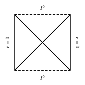
Figure 1: Maximally extended Penrose diagram of the de Sitter spacetime.

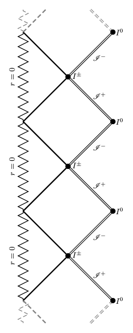
Figure 2: Maximally extended Penrose diagram of the extremal Reißner-Nordström spacetime.

Before studying the possible shell trajectories in the two geometries to identify the bounded ones, which we are interested in, we take full advantage of the parameter reduction implicit in the assumptions above, by passing to adimensional variables: this will be more convenient also for the subsequent numerical treatment. We thus choose to parametrize all the variables and constants in terms of the de Sitter cosmological horizon $H$ by setting

$$x=\frac{R}{H}\quad,\quad t=\frac{\tau}{H}\quad,\quad\Theta=\frac{Q}{H}\quad,\quad|\Theta|=\frac{M}{H}=\frac{m}{H}.$$ (14)

Then the quantities which are functions of $R$, become functions of $x$, all retaining their numerical values but $P$ and $S$, which are rescaled by $H$ and $H^{2}$ respectively:

$$\bar{P}(x;\Theta)=\frac{P(R;H,Q)}{H}\quad,\quad\bar{S}(\Theta)=\frac{S(H,Q)}{H^{2}}.$$ (15)

We thus have for the quantities evaluated along a classical trajectory, which are relevant in the study of the classical dynamics

$$\bar{f}_{\mathrm{in}}(x)=1-x^{2}$$ (16)

$$\bar{f}_{\mathrm{out}}(x)=1-\frac{2|\Theta|}{x}+\frac{\Theta^{2}}{x^{2}}$$ (17)

$$\bar{\sigma}_{\mathrm{in}}(x)=-\mathrm{Sign}\left(x^{3}-2|\Theta|\right)$$ (18)

$$\bar{\sigma}_{\mathrm{out}}(x)=-\mathrm{Sign}\left(x^{4}-2|\Theta|x+2\Theta^{2}\right)$$ (19)

$$\bar{V}(x)=-\frac{x^{2}\left(x^{4}-4|\Theta|x+4\Theta^{2}\right)}{4\Theta^{2}}$$ (20)

$$\bar{P}(x)=-x\tanh^{-1}\left\{\left(\frac{x\sqrt{x^{4}-4|\Theta|x+4\Theta^{2}}}{-x^{3}+2x-2|\Theta|}\right)^{\mathrm{Sign}\left\{\left(1-x^{2}\right)\left(x-|\Theta|\right)^{2}\right\}}\right\};$$ (21)

of course all can be expressed as functions of the single adimensional parameter $\Theta$.

Following [64, 75] we can study the classical dynamics in a compact way by means of a comprehensive graphical method fully exploiting the handy relation (9). It consists in plotting the potential $\bar{V}(x)$ together with the metric functions $\bar{f}_{\mathrm{in}}$, $\bar{f}_{\mathrm{out}}$. Then the allowed trajectories with the corresponding turning points can be determined looking at the segments of the $x$-axis (corresponding to zero energy), that are above the graph of the potential. In this diagram the points where the metric functions vanish, quickly help in determining if a classical path crosses the horizons of the external/internal geometry. Moreover the rescaled values of the radial coordinate $x$ for which $\sigma_{\mathrm{in/out}}$ changes sign are given, if they exist, by the values at which the metric function plots are tangent to the graph of the potential. This graphical information can be completed by the following analytical results.

Turning points of the potential

:
from (20) we see that the potential for $\Theta\neq 0$ has a (double) zero at $x=0$, so that it is regular at the origin, which is thus a trivial turning point of classical trajectories. Other turning points may, or may not, be present, depending on the value assumed by the parameter $\Theta$. Two cases are possible, as shown in figure 3.

Figure 3: Graph of the potential $\bar{V}(x)$ for different values of the parameter $\Theta$. Depending on the value of $\Theta$, the classical trajectory can have two non-vanishing turning points, or no non-vanishing turning points, as shown in the first and second figure, respectively. The in between case, which occurs for $\Theta=\Theta_{\mathrm{crit.}}=(3/4)^{3/2}$, is depicted in the third diagram.

Either there can be no other turning points, so that only a so called “bounce” classical trajectory exists (as is the case in figure 3 for $\Theta=0.7$), or there can be two more turning points so that in addition to the bounce trajectory there is also a bounded one (this is also shown in figure 3 for $\Theta=0.5$). As explicitly proved in A, the critical value for the parameter $\Theta$, $\Theta_{\mathrm{crit.}}=(3/4)^{3/2}$ gives the in between case, when the potential is tangent to the $x$ axis (third plot, again in figure 3). We thus see that only for $0<\Theta\leq\Theta_{\mathrm{crit.}}$ there are two non-vanishing turning points $x_{\mathrm{min}}$, $x_{\mathrm{max}}$ (actually with $x_{\mathrm{min}}\equiv x_{\mathrm{max}}$ if $\Theta=\Theta_{\mathrm{crit.}}$) and thus bounded solutions are allowed, the classical path being represented by the segment $[0,x_{\mathrm{min}}]$. We note that it is possible to find $x_{\mathrm{min}}$ and $x_{\mathrm{max}}$ in closed form solving the quartic equation that gives the non-vanishing solutions of $\bar{V}(x)=0$, and this (not very enlightening) expressions are reported in A.

Horizon positions with respect to the classical path

:
to correctly understand the spacetime geometry we also need the relative positions of the horizons with respect to the classical trajectories. This is also briefly discussed later on, but it is useful to report here a general result that can be deduced from figure 4, where for $0<\Theta\leq\Theta_{\mathrm{crit.}}$ the turning points, $0$, $x_{\mathrm{min}}$, $x_{\mathrm{max}}$ and the horizon of the exterior metric ($x(\Theta)=\Theta$) are plotted as functions of $\Theta$.

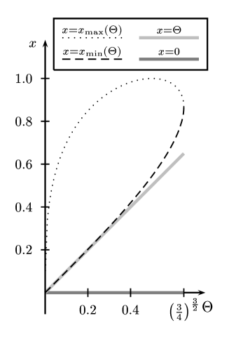
Figure 4: Graph of the non-negative roots ($x=0$, $x=x_{\mathrm{min}}(\Theta)$ and $x=x_{\mathrm{max}}(\Theta)$) of the potential $\bar{V}(x)$ together with the horizon $x=\Theta$ of the “out” Reißner-Nordström spacetime. Bounded trajectories are delimited by the $x=0$ line and the $x=x_{\mathrm{min}}(\Theta)$ curve, so that they always cross the horizon of the Reißner-Nordström spacetime, which the graph shows to be always smaller than $x=x_{\mathrm{min}}(\Theta)$.

It can be seen that the classical bounded trajectory, corresponding to the region between the $x$ axis and the $x_{\mathrm{min}}$ dashed curve, crosses for all values of $\Theta$ in the considered range the exterior horizon at $x=\Theta$. The horizon of the internal de Sitter domain (which is not plotted and corresponds to the horizontal line $x\equiv 1$ in rescaled variables) is instead never crossed by a bounded trajectory.

Asymptotic behaviour

:
quite generally, from (20) we also see that

$$\lim_{x\to+\infty}\bar{V}(x)=-\infty.$$ (22)

Regularity at the origin

:
the first and second derivatives of the potential are vanishing at $x=0$, $\rmd\bar{V}(x)/\rmd x=\rmd^{2}\bar{V}(x)/\rmd x^{2}=0$, and the third derivative is positive, $\rmd^{3}\bar{V}(x)/\rmd x^{3}=6/|\Theta|$, so that $x=0$ is a local maximum for $\bar{V}(x)$.

Thanks to the above properties, we can now perform the study of the classical dynamics for bounded trajectories by restricting the parameter $\Theta$ to the range

$$0<|\Theta|\leq\left(\frac{3}{4}\right)^{3/2},$$ (23)

where we have the general situation shown in figure 5. The figure shows, for $\Theta=0.55$, the potential $\bar{V}(x)$ together with $\bar{f}_{\mathrm{in}}(x)$ and $\bar{f}_{\mathrm{out}}(x)$. The classically allowed path is the thicker light gray segment on the $x$-axis.

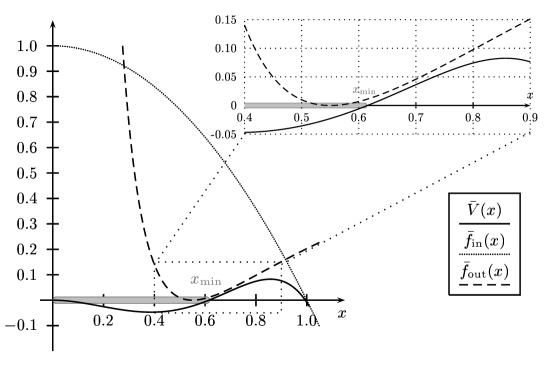
Figure 5: The graphical method to study the classical shell trajectories consists in plotting the potential $\bar{V}(x)$, together with the curves for the metric functions of the interior and of the exterior. The light gray path is a classically allowed bounded trajectory: as discussed in the text it crosses the horizon of the external geometry but no changes in the orientation of the normals occur along it.

Let us consider the dynamics in the de Sitter spacetime: the shell expands from vanishing radius up to a maximum (grayed path in the figure), which remains inside the de Sitter cosmological horizon, since, as can be seen, it is not crossed by the trajectory; then the shell shrinks back to zero radius. The sign of $\sigma_{\mathrm{in}}$ does not change along the trajectory, since as we can see always from figure 5, there are no points on the trajectory in which the plot of $\bar{f}_{\mathrm{in}}(x)$ is tangent to $\bar{V}(x)$: moreover, as can be easily verified, it is always positive, so that the trajectory crosses the left part of the de Sitter Penrose diagram. This is shown in figure 6, where the interior region is the shaded area, since for $\sigma_{\mathrm{in}}=+1$ the exterior normal is pointing to the right.

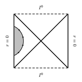
Figure 6: Penrose diagram of the de Sitter interior geometry with the bubble trajectory. The interior domain is the shaded region in the diagram.

In the same way we can perform the analysis in the Reißner-Nordström domain: we can see (in figure 5, but also from the above discussion about figure 4) that the bounded trajectory during the expansion from a vanishing radius, as well as during the following collapse, crosses the horizon of the exterior geometry. As before the sign of $\sigma_{\mathrm{out}}$ does not change along the trajectory (in the zoomed region of figure 5 we can more clearly see that the metric function graph is not tangent to the potential) and thus $\sigma_{\mathrm{out}}=-1$ always. If we draw the associated Penrose diagram, the exterior region is the shaded one in figure 7.

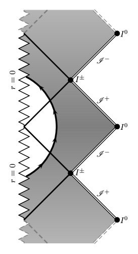
Figure 7: Penrose diagram of the Reißner-Nordström exterior geometry with the bubble trajectory. The exterior domain is the shaded region in the diagram.

The results shown above rest on two hypotheses, that we implicitly took for granted but which deserve a more detailed treatment.

The first one concerns the stability of the expanding and recollapsing shell against single particle decay: if the shell were not stable at the moment of time symmetry, then it would become thick and its trajectory would not be approximated by a sharp line (as depicted in figures 6 or 7). It is possible to show, following the treatment of [8] (please see B for details), that configurations stable against single particle decay of charged and/or uncharged particles actually exist.

The second issue is about possible changes of signs in $\sigma_{\mathrm{in}}$ or $\sigma_{\mathrm{out}}$, which would require a different analysis with respect to the one performed above. We also devote an appendix (C) to show that bounded trajectories are not affected by changes of sign in $\sigma_{\mathrm{in}}$ or $\sigma_{\mathrm{out}}$, so that the analysis performed above in a particular case is indeed valid in general.

With these remarks in mind, the complete spacetime manifold can now be confidently obtained by joining the interior with the exterior along the shell trajectory, i.e. joining the two shaded regions in figure 6 and figure 7 to get the final result shown in figure 8.

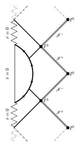
Figure 8: Penrose diagram of the de Sitter interior and the Reißner-Nordström exterior geometries joined along the bubble trajectory. It is obtained by joining the shaded regions of the two previous figures. The classical dynamics of this compound spacetime is described by Israel’s junction conditions and is discussed in detail in the text.

An observer inside the shell detects a non-vanishing cosmological constant. He lives as an observer inside a cosmological horizon. But as soon as he crosses the shell trajectory, he experiences a completely different situations: the cosmological constant suddenly vanishes and he can now detect a non-vanishing electric and gravitational field, as if outside a body with mass $M$ and charge $Q$ (with $M=|Q|$, because of our simplifying assumptions). We are now interested in studying the properties of this gravitational configuration when the system can be considered to be in a semi-classical quantum regime. For this we need an evaluation of the classical action along the classical trajectory of the shell.

4 Numerical evaluation of the classical action

As already anticipated in (12) we will evaluate the classical action as the integral of the classical momentum along a classically allowed trajectory. In our case, remembering the naming conventions about the zeros of $\bar{V}(x)$, this implies that the relevant turning points for the bounded trajectory in rescaled coordinates are $R_{1}/H\equiv x_{1}=0$ and $R_{2}/H\equiv x_{2}=x_{\mathrm{min}}$, so that

$$\bar{S}=\frac{S}{H^{2}}=2\int_{0}^{x_{\mathrm{min}}}\bar{P}(x)\rmd x$$

$$=-2\int_{0}^{x_{\mathrm{min}}}x\tanh^{-1}\left\{\left(\frac{x\sqrt{x^{4}-4|\Theta|x+4\Theta^{2}}}{-x^{3}+2x-2|\Theta|}\right)^{\mathrm{Sign}\left\{\left(1-x^{2}\right)\left(x-|\Theta|\right)^{2}\right\}}\right\}\rmd x.$$

The above integral has to be computed when the turning point $x_{\mathrm{min}}$ actually exists, i.e. in the range for $\Theta$ specified by (23). This means that the $\mathrm{Sign}$ at the exponent is always $+1$, and we can forget about it, so that the above turns into

$$\bar{S}=2\int_{0}^{x_{\mathrm{min}}}\bar{P}(x)\rmd x=2\int_{0}^{x_{\mathrm{min}}}x\tanh^{-1}\left\{\frac{x\sqrt{x^{4}-4|\Theta|x+4\Theta^{2}}}{x^{3}-2x+2|\Theta|}\right\}\rmd x.$$ (24)

We note that when $x=\Theta$, i.e. the shell is crossing a (double) zero of the external extremal Reißner-Nordström spacetime, the momentum is ill defined, since the argument of the inverse hyperbolic tangent is $-1$. $x=\Theta$ is thus a singularity on the integration path, but, being of the logarithmic type, it is integrable (the leading contribution to the singularity is determined in D).

The integral in (24) is not exactly computable analytically, but being reassured by the considerations above about its existence, the integration can be performed numerically. We have performed this kind of analysis with Mathematica^®, evaluating the integral numerically for $10000$ equally spaced test values of $\Theta$ in the interval $[10^{-4},(3/4)^{3/2}]$ and for other $10000$ test values in the interval $[10^{-16},10^{-4}]$ taken as a sequence converging to $0^{+}$ as $1/n^{4}$ for $n\to+\infty$. The final result is plotted in figure 9.

Figure 9: Graph of the functional dependence of the action from the $\Theta$ parameter as results from the numerical integration of (24) for $20000$ test values of $\Theta$ in the interval $[10^{-16},(3/4)^{3/2}]$ chosen as described in the text.

5 WKB Quantum States

We now assume that the system is in a quantum regime; we will perform its semiclassical quantization a la Bohr–Sommerfeld, i.e. considering the action as an integer multiple of $\hbar$. Remebering that all the computations of the previous section are in terms of the adimensional variables defined in (14) and (15), we have

$$S\left(Q,H\right)=H^{2}\bar{S}\left(\Theta\right)=H^{2}\bar{S}\left(\frac{Q}{H}\right),$$ (25)

so that we can rewrite the Bohr-Sommerfeld quantization condition as

$$S\left(Q,H\right)=l_{\mathrm{P}}^{2}n=n\quad,\quad n=0,1,2,\dots.$$ (26)

5.1 Preliminary Estimate

We first note that the quantization can be interpreted as giving a relation among the parameters of the model, in our case the charge $Q$ and the de Sitter cosmological horizon $H$. Let us take for example a total action of the order of the quantum, $l_{\mathrm{P}}^{2}$, i.e. associated to a state with quantum number $n=1$, for a de Sitter cosmological horizon $H=\sqrt{2}$. Then $\bar{S}\approx 1/2$, i.e. $\Theta=Q/H\approx 0.55$, so that $Q\approx 0.78$. This shows, as a preliminary estimate, that a small gravitational system with quantum properties is conceivable.

We can also see how the action behaves for variations of the parameters $Q$ and $H$ by a numerical plot of the level curves of the action. This is shown in figure 10.

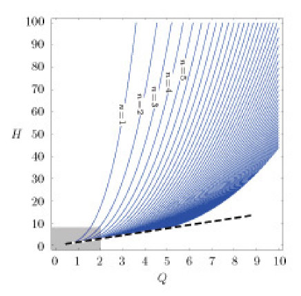
Figure 10: Graph of the level curves for the action for the level values $1,2,\dots,50$. The levels are obtained using the numerically evaluated action with the function ContourPlot of Mathematica^®. The thicker dashed black line displays the limit $H=(4/3)^{3/2}Q$ of the condition $Q/H>(3/4)^{3/2}$ for which bounded trajectories exist. The grayed region is shown, blew up, in figure 11.

To get a clearer plot in the region close to the limiting line $H=(4/3)^{3/2}Q$ for small $Q$, a smaller region of the plot is shown, enlarged, in figure 11.

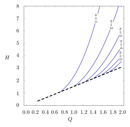
Figure 11: Blow up of the region of small $Q$, $H$ parameters. This better shows that the quantization condition implies a non-vanishing minimum allowed value for both the charge $Q$ and the de Sitter horizon $H$, i.e. a non-vanishing minimum allowed value for the charge $Q$ together with a maximum allowed value for the cosmological constant $1/H$.

5.2 Approximating the action

To get some analytical result we try to fit the $20000$ points for which we evaluated the action with some simple (polynomial) function. In this way we will be able to get an (approximated) relation among $Q$, $H$ and $n$. The choice of the approximating function is done with two goals in mind:

1. to approximate in the best possible way the behaviour of the action $\bar{S}$ at least in some regime;

2. to have a simple enough expression to get an algebraic relation among $Q$, $H$ and $n$.

To fulfill the above requirements we first analyze the leading $\Theta$ dependence of the action $\bar{S}$, expressed as the integral (24). From E we se that $\bar{P}(x)\sim x^{2}+\Or(x)^{2}$ and the upper turning point $x_{\mathrm{min}}(\Theta)\sim\Theta+\Or(\Theta)$, so that $\bar{S}(\Theta)\sim\Theta^{3}+\Or(\Theta)^{3}$. We thus choose an approximating function starting with a third power of $\Theta$ and having the next two powers of $\Theta$:

$$Ax^{5}+Bx^{4}+Cx^{3},$$ (27)

The coefficients $A$, $B$, $C$ in (27) have been determined from the $20000$ sample points using the function Regress of Mathematica^®, with the parameter IncludeConstant $\to$ False, since there is no constant term in the model: they result to be, together with the corresponding standard errors,

$$A=+10.11\pm 0.04$$

$$B=-7.39\pm 0.04$$ (28)

$$C=+3.64\pm 0.01,$$

with an adjusted regression coefficient of $0.99981$.
The comparison between approximated and numerical evaluated actions is plotted in figure 12.

Figure 12: Comparison between approximated and numerical evaluated actions. The expression $\bar{S}_{\mathrm{reg.}}(\Theta)$ is obtained, as described in the text, by a fit to a suitable polynomial. This figure aims to show that the main behaviour can be qualitatively approximated, but must not be taken to imply that the approximation is everywhere very good. Indeed when the action is very small, a very small approximation error can still give a relevant relative uncertainty.

Level curves of the approximated action are plotted in figure 13.

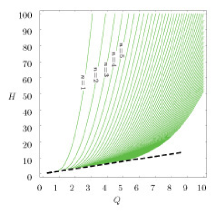
Figure 13: Graph of the level curves for the approximated action levels $1,2,\dots,50$. The levels are obtained using the approximating polynomial action with the function ContourPlot of Mathematica^®. The thicker dashed black line displays the limit $H=(4/3)^{3/2}Q$ of the condition $Q/H>(3/4)^{3/2}$ for which bounded trajectories exist.

From the approximated expression (27), which by (25) and (26) must equal $n$ when multiplied by $H^{2}$, we can get the following equation of the third degree in H,

$$AQ^{5}+BQ^{4}H+CQ^{3}H^{2}-nH^{3}=0:$$ (29)

this can be solved exactly to get the approximated relation for $H$ as a function of $Q$ and $n$ as it comes from the simplified expression (27) for the action. The quite complex algebraic expression is

$$H(Q;n)=\frac{CQ^{3}}{3n}+\frac{2^{1/3}H_{1}(Q;n)Q^{7/3}}{3n\sqrt[3]{H_{2}(Q;n)+\sqrt{4Q^{2}H_{1}^{3}(Q;n)+H_{2}^{2}(Q;n)}}}$$

$$-\frac{Q^{5/3}\sqrt[3]{H_{2}(Q;n)+\sqrt{4Q^{2}H_{1}^{3}(Q;n)+H_{2}^{2}(Q;n)}}}{2^{1/3}3n},$$ (30)

where

$$H_{1}(Q;n)=-C^{2}Q^{2}-3B_{1}n$$

$$H_{2}(Q;n)=-2C^{3}Q^{4}-9BCnQ^{2}-27A^{2}n^{2}$$

and the approximated relations above are only valid if

$$H>\frac{|Q|}{(3/4)^{3/2}},$$

a condition plainly coming from (23). The approximated levels of figure 13 are nothing but the graphs of the $n=\mathrm{const.}$ relations coming from (30).

6 Discussion

We have presented a model in which it is analyzed a general relativistic system composed of two spacetime domains, a de Sitter interior with cosmological horizon $H$ and an extremal Reißner-Nordström exterior with $M=|Q|$, joined across a thin shell of mass-energy $m=|Q|$. A semiclassical quantization of classically bounded trajectories can be performed using a scheme a la Bohr–Sommerfeld. In this way it is found that the quantum states can be characterized by a quantum number $n$, which is responsible for restricting the allowed values of $Q$ and $H$. In particular the quantum dynamics of the system constrains the values of $H$ as functions $H=H(Q;n)$, which we have approximated after a numerical analysis of the problem.

It is interesting to note that this is a sensible result in a semiclassical approximation to a quantum gravitational situations. Indeed a full quantum theory of gravity would treat the three-metric as a dynamical infinite-dimensional variable to be determined, say, by the Wheeler–deWitt equation in superspace. From our point of view, under the assumption we made, we are only in a minisuperspace approximation, since the functional form of the metric functions is fixed from the very beginning, leaving $H$ and $Q$ as the only free parameters: quantum gravity will thus impose condition on these quantities, i.e. determine the only residual degrees of freedom in the three geometry. We can also see from the enlarged plot of figure 11, that the quantization condition selects a minimum value for the allowed charge of the semiclassical quantized shell. At the same time, the cosmological constant of the interior region, cannot exceed a maximum value, which is also a sensible consequence of quantization. For a given fixed value of the ratio $Q/H=\bar{\kappa}$, which means that we are “moving” across the graphs of figures 10 and 11 along a line through the origin, we have discrete allowed values for $Q$ and $H$: these point are located on a parabola, since from (25) we exactly have $S(\bar{\kappa}H,H)=H^{2}\bar{S}(\bar{\kappa})$.

We also note that by the final result, systems characterized by different scales in the parameters can be described: among these, as expected, we find small scale systems (with a charge which is a small multiple of the elementary electron charge). Moreover an external asymptotic observer measures a total mass energy for the shell given by

$$E=m+\frac{1}{2}\left(\frac{Q^{2}}{r^{2}}-\frac{M^{2}}{r^{2}}\right)$$

which in our case is nothing but $E=m$, since $M^{2}=Q^{2}$: thus we effectively see in the outside domain an object with rest mass $m=|Q|$ and charge $Q$, which is the exterior manifestation of a bounded interior containing a part of spacetime characterized by a non-vanishing vacuum energy. Due to the form of the potential this bound semiclassical state is metastable, and will decay into an infinitely expanding shell after a finite time (a similar situation occurs in [81]), which in principle could be calculated (as proper time), studying the process of tunnelling across the classical effective potential barrier.

Appendix A Zeros of the potential and critical value of $\Theta$

The zeros of the potential $\bar{V}(x)$ can be obtained in closed form, since they are the zeroes of the numerator, i.e. the solutions of the equation

$$\bar{V}(x)=0\quad\Rightarrow\quad x^{2}(x^{4}-4ax+4a^{2})=0$$ (31)

with $a>0$ and $-x^{3}+2x-2a\neq 0$. We are interested in the non-negative solutions, which, apart from the $x=0$ one, can be determined exactly as solutions of the fourth order equation

$$x^{4}-4ax+4a^{2}=0.$$ (32)

By setting

$${\mathcal{B}}=\left\{9a^{2}+\left(81a^{4}-192a^{6}\right)^{1/2}\right\}^{1/3}$$

we have that for $0<a\leq(3/4)^{3/2}$

$$x_{\stackrel{{\scriptstyle\mathrm{\scriptstyle{}min}}}{{\mathrm{\scriptstyle{}max}}}}=\frac{1}{3^{1/3}2^{1/2}}\left\{\sqrt{\frac{4\cdot 3^{1/3}a^{2}}{{\mathcal{B}}}+{\mathcal{B}}}\mp\sqrt{-\frac{4\cdot 3^{1/3}a^{2}}{{\mathcal{B}}}-{{\mathcal{B}}}+\frac{6\cdot 2^{1/2}a}{\sqrt{\frac{4\cdot 3^{1/3}a^{2}}{{\mathcal{B}}}+{\mathcal{B}}}}}\right\}.$$ (33)

These expressions are not very enlightening: the one for $x_{\mathrm{min}}$ has been used to exactly evaluate the upper integration limit in the numerical evaluation of the integral that gives the classical action.

To see when the quartic part of the potential has two positive roots we can use the expression above, but also a smarter procedure, as follows. Clearly the limiting case is the one in which the potential is tangent to the positive $x$ axis, i.e. the two solutions coincide. In this case the quartic part must be of the form

$$(x-\alpha)^{2}(x^{2}+\beta x+\gamma)$$

$$=x^{4}+(\beta-2\alpha)x^{3}+(\gamma-2\alpha\beta+\alpha^{2})x^{2}+(\alpha\beta^{2}-2\alpha\gamma)x+\alpha^{2}\gamma,$$

which by comparison with $x^{4}-4ax-4a^{2}$ gives the set of equations

$$\left\{\matrix{\beta-2\alpha=0\hfill\cr\gamma-2\alpha\beta+\alpha^{2}=0\hfill\cr\alpha^{2}\beta-2\alpha\gamma=-4a\hfill\cr\alpha^{2}\gamma=4a^{2}\hfill}\right..$$

Then $\alpha=\beta/2$ and $\gamma=3\beta^{2}/4$ from the first two equations. This gives $\alpha=a^{1/3}$ from the third and $\alpha=(4a^{2}/3)^{1/4}$ from the fourth. These last two relations are compatible for non-vanishing $a$, if and only if $a=(3/4)^{3/2}$, which is thus the critical value of $a$.

Appendix B Stability of the shell against single particle decay

In this section we discuss the stability of the trajectory of the infinitesimally thin shell under single particle decay, following the treatment that can be found in [8]. The proof that the shell is stable against single particle decay of uncharged particles is not reproduced here, because it can be easily derived from the reference cited above, to which the reader is referred. We will instead shortly discuss the case in which charged particles are involved.

In more detail, the relevant question is if the motion of a charged particle, which at the instant of maximum expansion starts out where the shell is located, will subsequently be governed by a confining, i.e. “$\cup$-shaped”, effective potential, or not. Performing the analysis at the instant of maximum expansion, where the potential is static, simplifies the computation: subsequent changes of the potential will have, anyway, only adiabatic effects on the locally trapped particle and this is not relevant for the point under discussion. To get the desired result we will proceed in two steps:

1. identify the effective potential governing the motion of a particle in the exterior Reißner-Nordström geometry;

2. evaluate if it is “$\cup$-” or “$\cap$-shaped” at the point of maximum expansion.

We will work in the adimensional units used throughout the rest of the paper.

B.1 Effective potential for a charged particle in the Reißner-Nordström spacetime

The effective potential for the motion of a particle of charge $q$ and mass $\mu$ in the Reißner-Nordström spacetime can be obtained in many different ways. Probably the quickest one is to start from the more general result that can be found in the equation after equation (3) in Box 33.5 of [70], i.e. the effective potential for the orbits of test particles in the equatorial plane of a Kerr-Newman black hole. Specializing this result to a black hole with zero angular momentum we obtain the effective potential in the Reißner-Nordström case. Perhaps more instructive is to perform again the analysis until equation (6) of [8] adding the electrostatic contribution to the particle momentum or solving the Hamilton-Jacobi equation in the Reißner-Nordström metric. Anyway, the final result for the extremal case we are interested in is

$$\tilde{V}(x)=\frac{\tilde{\epsilon}\Theta}{x}+\left(1-\frac{\Theta}{x}\right)\left(1+\frac{\tilde{\lambda}^{2}}{x^{2}}\right)^{1/2},$$ (34)

where $\tilde{\epsilon}$ is the charge/mass ratio of the test particle and $\tilde{\lambda}=\tilde{L}/H$ is its angular momentum per unit mass ($\tilde{L}=L/\mu)$ in the $H$ scale defined in (14) and (15).

B.2 Evaluation of the Effective Potential at the point of maximum expansion

With the above results at hand, we now evaluate the second derivative of the effective potential, i.e.

$$\tilde{V}(x)^{\prime\prime}=\frac{3x^{2}\tilde{\lambda}^{2}+2\tilde{\lambda}^{4}+2\tilde{\epsilon}\Theta\left(x^{2}+\tilde{\lambda^{2}}\right)^{3/2}-(2x^{4}+9x^{2}\tilde{\lambda}^{2}+6\tilde{\lambda}^{4})|\Theta|}{x^{3}\left(x^{2}+\tilde{\lambda^{2}}\right)^{3/2}};$$ (35)

we are interested in its sign at the value $x_{\mathrm{min}}$, the maximum radius of the shell given in (33): a positive sign will indicate that the potential is “$\cup$-shaped” and thus the shell stable. To get the result, we can restrict the study to the numerator $\tilde{N}(x_{\mathrm{min}})$ of (35),

$$\tilde{N}(x_{\mathrm{min}})=3x_{\mathrm{min}}^{2}\tilde{\lambda}^{2}+2\tilde{\lambda}^{4}+2\tilde{\epsilon}\Theta\left(x^{2}_{\mathrm{min}}+\tilde{\lambda^{2}}\right)^{3/2}-(2x_{\mathrm{min}}^{4}+9x_{\mathrm{min}}^{2}\tilde{\lambda}^{2}+6\tilde{\lambda}^{4})|\Theta|,$$

since the denominator does not contribute to the sign. We also remember that the quantity $x_{\mathrm{min}}$ depends on $\Theta$, since (31) comes from (20) with $a=|\Theta|$.

Even with the above simplification, the detailed study of the sign of the quantity under consideration is complicated, mainly because of the non-trivial $\Theta$ dependence; a graphical analysis is also of little help, since $\tilde{N}(x_{\mathrm{min}})$ depends on the three variables $\Theta$, $\tilde{\epsilon}$ and $\tilde{\lambda}$, namely the adimensional charge $Q/H$, the charge/mass ratio $q/\mu$ of the test particle and the adimensional angular momentum per unit mass $L/(H\mu)$ of the test particle. Thus we will not search for the most general result, i.e. we will not give necessary and sufficient conditions for the stability of the shell; we will show, instead, that in some physically reasonable situations the shell itself is indeed stable against single charged particle decay.

In particular we see that in the units we are using, the adimensional parameter $\tilde{\epsilon}$ is a large number, i.e. the charge/mass ratio for an elementary particle is very large. Thus we consider the behaviour of the numerator for large $\tilde{\epsilon}$:

$$\lim_{\tilde{\epsilon}\to\infty}\tilde{N}(x_{\mathrm{min}})=+\infty;$$

the limit has always the “$+$” sign, since we consider emission of charges of the same sign of those composing the shell; thus in this limit the second derivative of the effective potential is positive, which shows stability under charged elementary particle decay.

As a second case, we see what happens for radial emission of particles:

$$\lim_{\tilde{\lambda}\to 0}\tilde{N}(x_{\mathrm{min}})=2x_{\mathrm{min}}^{3}|\Theta|(|\tilde{\epsilon}|-x_{\mathrm{min}});$$

we again used the fact that ejected particles have the same charge as the shell, so that $\tilde{\epsilon}\Theta=|\tilde{\epsilon}|\cdot|\Theta|$. In this case also we see that, for elementary particle emission, we certainly can realize the situation $\tilde{\epsilon}>x_{\mathrm{min}}$, so the sign is again positive.

Even restricting the study to the two cases above, we can thus conclude that, shell configurations which are stable against single particle decay can be realized.

Appendix C General analysis for $\sigma_{\mathrm{in}}$, $\sigma_{\mathrm{out}}$ on a bounded trajectory

The “graphical” analysis of the classical dynamics performed in section 3 is based on the plot of figure 5. In the discussion a relevant point is the sign of $\bar{\sigma}_{\mathrm{in}}$ and $\bar{\sigma}_{\mathrm{out}}$, which is crucial in determining the direction of the normal to the shell pointing in the direction of increasing radius as well as the side of the Penrose diagram crossed by the trajectory. We will show here that the situation analyzed for the particular value $\Theta=0.55$ is, in fact, general. The sign of $\bar{\sigma}_{\mathrm{in}}$ is given (18), so that we see that is positive for

$$x<x_{\sigma_{\mathrm{in}}}(\Theta)\equiv(2\Theta)^{1/3}.$$

More complicate is the analysis of the sign of $\bar{\sigma}_{\mathrm{out}}$, because from (19) we see that it is determined as the sign of a polynomial of order four. It has at most two real roots for $\Theta<\Theta_{\mathrm{crit.}}/\sqrt{2}=(3/4)^{3/2}/\sqrt{2}$; this can be seen also from the analysis of A. Indeed $\bar{\sigma}_{out}>0$ if

$$x^{4}-2ax+2a^{2}<0\quad\mathrm{with}\quad a>0.$$

The real roots of the left hand side of the above inequality can be deduced from those of the left hand side of (32) since

$$x^{4}-2ax+2a^{2}\longrightarrow\frac{1}{4}\left(x^{4}-4ax+4a^{2}\right)\quad{\mathrm{when}}\quad x\to\frac{x}{\sqrt{2}}\quad\mathrm{and}\quad a\to\frac{a}{\sqrt{2}}.$$

Then, if we call $x_{\sigma_{\mathrm{out}}}^{(-)}$ and $x_{\sigma_{\mathrm{out}}}^{(+)}$ the two real values for which $\bar{\sigma}_{\mathrm{out}}$ changes sign, we see, using the transformation above, that we must have $a\leq(3/4)^{3/2}/\sqrt{2}$ and that

$$x_{\sigma_{\mathrm{out}}}^{(\mp)}=\frac{1}{2\cdot 3^{1/3}}\left\{\sqrt{\frac{8\cdot 3^{1/3}b^{2}}{{\mathcal{T}}}+{\mathcal{T}}}\mp\sqrt{-\frac{8\cdot{3^{1/3}}b^{2}}{{\mathcal{T}}}-{\mathcal{T}}+\frac{12b}{\sqrt{\frac{8\cdot 3^{1/3}b^{2}}{{\mathcal{T}}}+{\mathcal{T}}}}}\right\}$$ (36)

with

$${\mathcal{T}}=\sqrt[3]{18b^{2}+2\sqrt{81b^{4}-384b^{6}}}$$

Since the above expressions are not very enlightening (and the same is true for those of (33)), the easiest way to compare them with the turning points is again the graphical one, i.e. the plot of $x_{\sigma_{\mathrm{in}}}(\Theta)$, $x_{\sigma_{\mathrm{out}}}^{(\pm)}(\Theta)$, $x_{\mathrm{min}}(\Theta)$, $x_{\mathrm{max}}(\Theta)$, which we can see in figure 14.

Figure 14: Graph of the curves that helps in determining the sign of $\sigma$’s for different values of the parameter $\Theta$. Since the classically allowed trajectories are delimited by the $x=0$ axis and by the dark gray continuous curve $x=x_{\mathrm{min.}}(\Theta)$, we see that no changes of signs of $sigma$’s occur along them.

For small $x$ (on the vertical axis) $\bar{\sigma}_{\mathrm{in}}$ is positive and $\bar{\sigma}_{\mathrm{out}}$ is negative. Since all the zeroes, when they exist, are bigger than the the turning point $x_{\mathrm{min}}$, which is the upper limit of the bounded trajectory, then there is no change of sign of $\sigma$’s along it.

Appendix D Character of the singularity on the integration path

In this section we determine the leading contribution to the logarithmic (and thus integrable) singularity on the integration path that appears in the evaluation of the integral in (24). The logarithmic character stems from the definition of the inverse hyperbolic tangent in terms of the logarithm and from the fact that its argument is a rational function with the following properties:

$$\lim_{x\to|\Theta|}{\mathcal{F}(x;\Theta)}\equiv\lim_{x\to|\Theta|}\frac{{\mathcal{R}}^{1/2}(x;\Theta)}{{\mathcal{D}}(x;\Theta)}\equiv\lim_{x\to|\Theta|}\frac{x\sqrt{x^{4}-4|\Theta|x+4\Theta^{2}}}{x^{3}-2x+2|\Theta|}=1,$$

i.e.

$${\mathcal{F}}(|\Theta|;\Theta)=1$$ (37)

To extract the behaviour of the above function around the point $x=|\Theta|$ we develop it in power series. Let us set

$${\mathcal{R}}(x;\Theta)=x^{6}-4|\Theta|x^{3}+4\Theta^{2}x^{2}\quad\mathrm{with}\quad{\mathcal{R}}(|\Theta|;\Theta)=\Theta^{6}$$ (38)

$${\mathcal{D}}(x;\Theta)=x^{3}-2x+2|\Theta|\quad\mathrm{with}\quad{\mathcal{D}}(|\Theta|;\Theta)=|\Theta|^{3}.$$ (39)

Then it follows

$${\mathcal{R}}^{\prime}(x;\Theta)=6x^{5}-12|\Theta|x^{2}+8\Theta^{2}x\quad\mathrm{so\ that}\quad{\mathcal{R}}^{\prime}(|\Theta|;\Theta)=6|\Theta|^{5}-4|\Theta|^{3}$$ (40)

$${\mathcal{D}}^{\prime}(x;\Theta)=3x^{2}-2\quad\mathrm{so\ that}\quad{\mathcal{D}}^{\prime}(|\Theta|;\Theta)=3\Theta^{2}-2.$$ (41)

and

$${\mathcal{R}}^{\prime\prime}(x;\Theta)=30x^{4}-24|\Theta|x+8\Theta^{2}\quad\mathrm{so\ that}\quad{\mathcal{R}}^{\prime\prime}(|\Theta|;\Theta)=30\Theta^{4}-16\Theta^{2}$$ (42)

$${\mathcal{D}}^{\prime\prime}(x;\Theta)=6x\quad\mathrm{so\ that}\quad{\mathcal{D}}^{\prime\prime}(|\Theta|;\Theta)=6|\Theta|.$$ (43)

We then compute ${\mathcal{F}}^{\prime}(|\Theta|;\Theta)$ and ${\mathcal{F}}^{\prime\prime}(|\Theta|;\Theta)$, i.e. the first and second derivatives of the argument of the inverse hyperbolic tangent. Since

$${\mathcal{F}}^{\prime}=\frac{{\mathcal{R}}^{\prime}{\mathcal{D}}-2{\mathcal{R}}{\mathcal{D}}^{\prime}}{2{\mathcal{R}}^{1/2}{\mathcal{D}}^{2}}$$

we obtain

$${\mathcal{F}}^{\prime}(|\Theta|;\Theta)=0.$$ (44)

Moreover

$${\mathcal{F}}^{\prime\prime}=\frac{2\left({\mathcal{R}}^{\prime\prime}{\mathcal{D}}-{\mathcal{R}}^{\prime}{\mathcal{D}}^{\prime}-2{\mathcal{R}}{\mathcal{D}}^{\prime\prime}\right){\mathcal{R}}{\mathcal{D}}-\left({\mathcal{R}}^{\prime}{\mathcal{D}}-2{\mathcal{R}}{\mathcal{D}}^{\prime}\right)\left({\mathcal{R}}^{\prime}{\mathcal{D}}+4{\mathcal{R}}{\mathcal{D}}^{\prime}\right)}{4{\mathcal{R}}^{3/2}{\mathcal{D}}^{3}}$$

and we get

$${\mathcal{F}}^{\prime\prime}(|\Theta|;\Theta)=-\frac{4}{\Theta^{6}}\left(1-\Theta^{2}\right).$$ (45)

The expansion of ${\mathcal{F}}$ around $x=|\Theta|$ up to second order can then be written, using (37), (44) and (45), as

$${\mathcal{F}}(x;\Theta)=1-\frac{2\left(1-\Theta^{2}\right)}{\Theta^{6}}\left(x-|\Theta|\right)^{2}+\Or\left(x-|\Theta|\right)^{3}$$

and inserting this result inside the expression of the hyperbolic tangent in terms of logarithms, we can easily see, as expected, that the singularity is integrable.

Appendix E $\Theta$ dependence of the Action

We consider the action integral (24). Expanding the integrand we get

$$x\tanh^{-1}\left\{\frac{x\sqrt{x^{4}-4|\Theta|x+4\Theta^{2}}}{x^{3}-2x+2|\Theta|}\right\}=x^{2}+\frac{1}{2|\Theta|}x^{3}+\Or(x^{4});$$

Then the upper integration limit, $x(\Theta)$, can be expanded as

$$x(\Theta)=\Theta+\Or(\Theta^{2})$$

so that when both expansions hold, we can write

$$\bar{S}(\Theta)\sim\frac{11|\Theta|^{3}}{12}+\Or(\Theta^{4}).$$

We thus see that the leading term for small $|\Theta|$ is $\sim|\Theta^{3}|$.

References

References

- [1] Israel W 1966 Nuovo Cimento B XLIV B 1
- [2] Israel W 1967 Nuovo Cimento B 48 463(E)
- [3] Barrabès C and Israel W 1991 Phys. Rev. D 43 1129
- [4] Jezierski J, Kijowski J and Czuchry E 2000 Rep. Math. Phys. 46 399
- [5] Jezierski J, Kijowski J and Czuchry E 2002 Phys. Rev. D 65 064036
- [6] Louko J, Whiting B F and Friedman J L 1998 Phys. Rev. D 57 2279
- [7] Kuchař K V 1994 Phys. Rev. D 50 3961
- [8] Gerlach U H 1970 Phys. Rev. Lett. 25 1771
- [9] Núñez D 1997 Astrophys. J. 482 963
- [10] Núñez D and deOliveira H P 1996 Phys. Lett. A 214 227
- [11] Frauendiener J and Klein C 1995 J. Math. Phys. 36 3632
- [12] Wang A Z 2001 Braz. J. Phys. 31 188
- [13] Martín-García J M and Gundlach C 2001 Phys. Rev. D 6402 024012
- [14] Alberghi G L, Casadio R, Vacca G P and Venturi G 1999 Class. Quantum Grav. 16 131
- [15] delaCruz V and Israel W 1967 Nuovo Cimento LI A 744
- [16] Kuchař K 1968 Czech. J. Phys. 18 435
- [17] Chase J E 1970 Nuovo Cimento LXVII B 136
- [18] Matravers D R and Humphreys N P 2001 Gen. Relativ. Gravit. 33 531
- [19] Ribeiro M B 1992 Astrophys. J. 388 1
- [20] Berezin V A, Kuzmin V A and Tkachev I I 1987 Phys. Rev. D 36 2919
- [21] Doležel T, Bičák J and Deruelle N 2000 Class. Quantum Grav. 17 2719
- [22] Farhi E, Guth A H and Guven J 1990 Nucl. Phys. B 339 417
- [23] Guth A H 1991 Phys. Scr. T36 237
- [24] Mishima T, Suzuki H and Yoshino N 1997 Class. Quantum Grav. 14 2179
- [25] Dolgov A D and Khriplovich I B 1997 Phys. Lett. B 400 12
- [26] Berezin V A, Kozimirov N G, Kuzmin V A and Tkachev I I 1988 Phys. Lett. B 212 415
- [27] Hájíček B, Kay S and Kuchař K V 1992 Phys. Rev. D 46 5439
- [28] Berezin V A 1990 Phys. Lett. B 241 194
- [29] Berezin V A 2002 Int. J. Mod. Phys. A 17 979
- [30] Berezin V A 1996 Int. J. Mod. Phys. D 5 679
- [31] Nakamura K, Oshiro Y and Tomimatsu A 1996 Phys. Rev. D 53 4356
- [32] Visser M 1989 Nucl. Phys. B 328 203
- [33] Visser M 1991 Phys. Rev. D 43 402
- [34] Hochberg D 1995 Phys. Rev. D 52 6846
- [35] Visser M 1995 Lorentzian wormholes: from Einstein to Hawking (Woodbury: American institute of Physics)
- [36] Poisson E and Visser M 1995 Phys. Rev. D 52 7318
- [37] Visser M 1990 Phys. Lett. B 242 24
- [38] Redmount I H and Suen W M 1994 Phys. Rev. D 49 5199
- [39] Visser M 1994 Phys. Rev. D 49 3963
- [40] Kraus P and Wilczek F 1995 Nucl. Phys. B 433 403
- [41] Berezin V A 1997 Phys. Rev. D 55 2139
- [42] Hochberg D and Kephart T W 1993 Phys. Rev. Lett. 70 2665
- [43] Hájíček P and Kijowski J 2000 Phys. Rev. D 6204 044025
- [44] Katz J and Ori A 1990 Class. Quantum Grav. 7 787
- [45] Martinez E A 1996 Phys. Rev. D 53 7062
- [46] Alberghi G L, Casadio R and Venturi G 1999 Phys. Rev. D 6012 124018
- [47] Guendelman E I 1991 Gen. Relativ. Gravit. 23 1415
- [48] Georgiou A 1994 Class. Quantum Grav. 11 167
- [49] Pereira P R C T and Wang A Z 2000 Gen. Relativ. Gravit. 32 2189
- [50] Pereira P R C T and Wang A Z 2000 Phys. Rev. D 6212 124001
- [51] Hájíček P and Bičák J 1997 Phys. Rev. D 56 4706
- [52] Friedman J L, Louko J and Winters-Hilt S N 1997 Phys. Rev. D 56 7674
- [53] Hájíček P and Kijowski J 1998 Phys. Rev. D 57 914
- [54] Hájíček P 1999 J. Math. Phys. 40 318
- [55] Hájíček P 1998 Phys. Rev. D 57 936
- [56] Kijowski J 1998 Acta Phys. Pol. B 29 1001
- [57] Gladush V D 2001 J. Math. Phys. 42 2590
- [58] Mukohyama S 2002 Phys. Rev. D 6502 024028
- [59] Hájíček P 1998 Phys. Rev. D 58 084005
- [60] Barceló C and Visser M 2000 Phys. Lett. B 482 183
- [61] Gogberashvili M 2000 Europhys. Lett. 49 396
- [62] Anchordoqui L A and Bergliaffa S E P 2000 Phys. Rev. D 6206 067502
- [63] Barceló C and Visser M 2000 Nucl. Phys. B 584 415
- [64] Blau S K, Guendelman E I and Guth A H 1987 Phys. Rev. D 35 1747
- [65] Yamanaka Y, Nakao K and Sato H 1992 Prog. Theor. Phys. 88 1097
- [66] Balbinot R, Barrabès C and Fabbri A 1994 Phys. Rev. D 49 2801
- [67] Zloshchastiev K G 1998 Phys. Rev. D 57 4812
- [68] DeSitter W 1917 Proc. Kon. Ned. Akad. Wet. 19 1217
- [69] DeSitter W 1917 Proc. Kon. Ned. Akad. Wet. 20 229
- [70] Misner C M, Thorne K S and Thorne K S 1970 Gravitation (San Francisco: W. H. Freeman and Company)
- [71] Reißner H 1916 Ann. Phys. (Germany) 50 106
- [72] Nordström G 1918 Proc. Kon. Ned. Akad. Wet. 20 1238
- [73] Ansoldi S, Aurilia A, Balbinot R and Spallucci E 1997 Class. Quantum Grav. 14 2727
- [74] Ansoldi S 1994 Nucleazione quantogravitazionale di dominii spaziotemporali (Graduation Thesis, 169 pages, Department of Theoretical Physics of the University of Trieste - Trieste - Italy, in Italian)
- [75] Aurilia A, Palmer M and Spallucci E 1989 Phys. Rev. D 40 2511
- [76] Mehra J and Rechenberg H 1982 The historical development of quantum theory 133 Vol 1 (New York: Springer Verlag) and references therein.
- [77] Ansoldi S, Aurilia A, Balbinot R and Spallucci E 1996 Physics Essay 9 556
- [78] Coleman S and de Luccia F 1980 Phys Rev D 21 3305
- [79] Parke S 1983 Phys. Lett. B 121 313
- [80] Carter B 1966 Phys. Lett. 21 423
- [81] Guendelman E I and Portnoy J 1999 Class. Quantum Grav. 16 3315