Decay of spin-1/2 field around Reissner-Nordstrom black hole

Abstract

To find what influence the charge of the black hole $Q$ will bring to the evolution of the quasinormal modes, we calculate the quasinormal frequencies of the neutrino field (charge $e=0$) perturbations and those of the massless Dirac field ($e\neq 0$) perturbations in the RN metric. The influences of $Q$, $e$, the momentum quantum number $l$, and the mode number $n$ are discussed. Among the conclusions, the most important one is that, at the stage of quasinormal ringing, the larger when the black hole and the field have the same kind of charge ($eQ>0$), the quasinormal modes of the massless charged Dirac field decay faster than those of the neutral ones, and when $eQ<0$, the massless charged Dirac field decays slower.

I Introduction

It is well known that black holes and neutron stars have their characteristic ”sound”: quasinormal modes, which were originally found to play a prominent role in the gravitational radiation theoretically and were hoped to be detected in the gravitational experiments (seeK.Kokkotas ; Hans and references therein for review). They have been extensively studied recently for their possible connection with the quantum gravity through an observation made by Dreyer in Ref. Dreyer , where the author fixed the free parameter $\gamma$ of Loop Quantum Gravity(LQG) and suggested the gauge group of LQG may be $SO(3)$ rather than $SU(2)$. This is remarkableBaez and surely makes a good example of utilizing the macroscopic behavior of black holes to deduce their microscopic nature.

Besides the application in LQG, the quasinormal modes are also used in many other fields, especially the Anti-de sitter/Conformal Field Theory (AdS/CFT) correspondenceBirm . In Ref. Horowitz , from the AdS/CFT correspondence, the quasinormal modes of the AdS black hole are used to determine the relaxation time of a field perturbation, i.e., the imaginary part of the quasinormal frequency is proportional to the inverse of the damping time of a given mode. Hod and PiranHod considered the behavior of a charged scalar field perturbation and found that, its quasinormal modes will dominate the radiation in the late time evolution for their slower decay than the neutral ones. Konoplya, in his workKonoplya , first investigated a complex (charged) scalar field perturbation through calculating its quasinormal modes in the Reissner-Nordstrom (RN), RNAdS and dialton black holes and found that, on the contrary, the neutral perturbations will decay slower than the charged ones at the stage of quasinormal ringing. In this paper, we turn to treat the spin $1/2$ Dirac particles, in the presence of the RN black holes with charge $Q$. Calculating quasinormal frequencies of the neutrino field (charge $e=0$) perturbations and those of the massless Dirac field (charge $e\neq 0$) perturbations in the RN metric, we found that when the product $eQ$ is positive, the quasinormal modes of the massless Dirac field decay faster than those of the neutral ones and when $eQ$ is negative, the perturbations of the massless Dirac field decay slower than those of the neutral field. The detailed discussions can be found in the following sections.

In Sec. II, in the RN metric, we will calculate the quasinormal frequencies of the neutrino field perturbations and those of the massless Dirac field perturbations. In Sec. III, with some figures and tables, we show clearly what influence the charge of the black hole brings to the behavior of the quasinormal modes, including the energy and the decay rate. Sec. IV is a summary with some suggestions about the future research.

II Quasinormal modes in RN metric

We shall calculate the quasinormal frequencies of the massless Dirac field perturbations and the neutrino field perturbations in the RN metric

$$ds^{2}=-\left(1-\frac{2M}{r}+\frac{Q^{2}}{r^{2}}\right)dt^{2}+\left(1-\frac{2M}{r}+\frac{Q^{2}}{r^{2}}\right)^{-1}dr^{2}+r^{2}\left(d\theta^{2}+\sin^{2}\theta d\phi^{2}\right).$$ (1)

The wave equation can be written as

$$[\gamma^{a}e_{a}^{~{}\mu}(\partial_{\mu}+\Gamma_{\mu}+eA_{\mu})]\Psi=0.$$ (2)

In Eq. (2), $\gamma^{a}$ are the Dirac matrices with the forms

$$\gamma^{0}=\left(\begin{array}[]{cc}-i&0\\ 0&i\end{array}\right),~{}\gamma^{i}=\left(\begin{array}[]{cc}0&-i\sigma^{i}\\ i\sigma^{i}&0\end{array}\right),~{}\left(i=1,2,3\right),$$

where $\sigma^{i}$ are the Pauli matrices. $e_{a}^{~{}\mu}$ is the inverse of the tetrad $e_{\mu}^{~{}a}$ defined by the spacetime metric

$$g_{\mu\nu}=\eta_{ab}e_{\mu}^{~{}a}e_{\nu}^{~{}b},\ \eta_{ab}=diag(-1,1,1,1).$$

$\Gamma_{\mu}$ are the spin connection given by

$$\Gamma_{\mu}=\frac{1}{8}\left[\gamma^{a},\gamma^{b}\right]e_{a}^{~{}\nu}e_{b\nu;\mu},\ e_{b\nu;\mu}=\partial_{\mu}e_{b\nu}-\Gamma_{\mu\nu}^{a}e_{ba},$$

where $\Gamma_{\mu\nu}^{a}$ are the Christoffel symbols. And, $eA_{\mu}$ is the electromagnetic potential of the black hole.

In the following discussions, we adopt the natural unit, $\hbar=c=G=4\pi\varepsilon_{0}=1$. It means that all physical quantities, such as mass, length, charge, time, energy, and so on, are dimensionless. The following replacing relations can be used to restore all of them:

Mass $$: \text{ }m\rightarrow\left(\frac{c\hbar}{G}\right)^{-1/2}m=\frac{m}{m_{p}},\quad m_{p}=\sqrt{\frac{c\hbar}{G}},$$

Length $$: \text{ }l\rightarrow\left(\frac{\hbar G}{c^{3}}\right)^{-1/2}l=\frac{l}{l_{p}},\quad l_{p}=\sqrt{\frac{\hbar G}{c^{3}}},$$

Time $$: \text{ }t\rightarrow\left(\frac{\hbar G}{c^{5}}\right)^{-1/2}t=\frac{t}{t_{p}},\quad t_{p}=\sqrt{\frac{\hbar G}{c^{5}}},$$

Charge $$: \text{ }e\rightarrow\left(4\pi\varepsilon_{0}c\hbar\right)^{-1/2}e=\frac{e}{e_{p}},\quad e_{p}=\sqrt{4\pi\varepsilon_{0}c\hbar},$$

Energy $$: \text{ }E\rightarrow\left(\frac{c^{5}\hbar}{G}\right)^{-1/2}E=\frac{E}{E_{p}},\quad E_{p}=\sqrt{\frac{c^{5}\hbar}{G}}.$$

For the RN spacetime, the electromagnetic potential $eA_{\mu}$ can be written as

$$eA_{\mu}=\left(\frac{eQ}{r},0,0,0\right),$$ (3)

where $Q$ is the charge of the RN black hole, and $e$ is zero for neutrinos and nonzero for Dirac particles. In the following we shall see that we can just consider the sign of the product $eQ$ without taking into consideration the sign of each quantity respectively. Therefore, for convenience we shall take $Q$ to be always positive and only switch the sign of $e$, when we are studying the influence of the charge of the black hole on the quasinormal frequencies of the Dirac field perturbations.

For the RN spacetime, we can select the tetrad $e_{\mu}^{~{}a}$ as

$$e_{\mu}^{~{}a}=diag\left(\left(1-\frac{2M}{r}+\frac{Q^{2}}{r^{2}}\right)^{1/2},\left(1-\frac{2M}{r}+\frac{Q^{2}}{r^{2}}\right)^{-1/2},r,r\sin\theta\right).$$ (4)

Using the ansatz Cho ,

$$\Phi(t,r,\theta,\phi)=\left(\begin{array}[]{l}\frac{iG^{(\pm)}(r)}{r}\varphi_{jm}^{(\pm)}(\theta,\phi)\\ \frac{F^{(\pm)}(r)}{r}\varphi_{jm}^{(\pm)}(\theta,\phi)\end{array}\right)e^{-iEt},$$ (5)

where for $j=l+1/2$,

$$\varphi_{jm}^{(+)}=\left(\begin{array}[]{l}\sqrt{\frac{l+1/2+m}{2l+1}}Y_{l}^{m-1/2}\\ \sqrt{\frac{l+1/2-m}{2l+1}}Y_{l}^{m+1/2}\end{array}\right),$$

and for $j=l-1/2$,

$$\varphi_{jm}^{(-)}=\left(\begin{array}[]{l}\sqrt{\frac{l+1/2-m}{2l+1}}Y_{l}^{m-1/2}\\ -\sqrt{\frac{l+1/2+m}{2l+1}}Y_{l}^{m+1/2}\end{array}\right),$$

we can get the radial part of the wave equation

$$\left(-\frac{d^{2}}{dr_{*}^{2}}+V_{1}\right)F=\omega^{2}F,$$ (6)

and

$$\left(-\frac{d^{2}}{dr_{*}^{2}}+V_{2}\right)G=\omega^{2}G,$$ (7)

where

$$\frac{dr_{*}}{dr}=\left(1-\frac{2M}{r}+\frac{Q^{2}}{r^{2}}\right)^{-1}.$$

$V_{1,2}$ can be expressed as

$$V_{1,2}(r,k)=\pm\frac{dW}{dr_{*}}+W^{2},$$ (8)

with

$$W=\left(1-\frac{2M}{r}+\frac{Q^{2}}{r^{2}}\right)^{\frac{1}{2}}\frac{\mid k\mid}{r}-\frac{eQ}{r},$$ (9)

where $k$ equals $l$ in the ($+$) case and $-\left(l+1\right)$ in the ($-$) case, and the momentum quantum number $l$ is a non-negative integer. One may notice that $V_{1}$ and $V_{2}$ are supersymmetric partners of the superpotential $W$super , and they will give the same quasinormal frequencies. So, in the following work, we only discuss the $V_{1}(+)$ case where the momentum quantum number $l$ equals $k$.

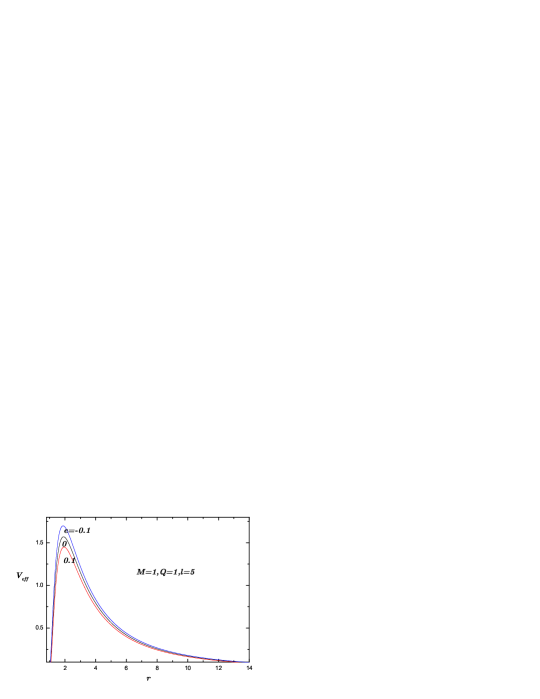
Figure 1: The effective potential barrier of $e=0$, $\pm 0.1$ with $l=5$, $M=1$, $Q=1$.

Fig. 1 shows the potential barrier of the three cases mentioned above with the maximal values

$$V_{\max}(l=5,e=0.1,Q=1)=1.441,$$

$$V_{\max}(l=5,e=-0.1,Q=1)=1.689,$$

$$V_{\max}(l=5,e=0,Q=1)=1.545,$$

which can be derived from Eq. (8). And from Fig. 2, we can see the peak of the potential barrier increases with $l$ and its position $r$ approaches a limit.

To evaluate the quasinormal frequencies, we adopt the third-order WKB approximation, which was originally proposed by Schutz, Iyer and WillSchutz and recently developed by Konoplya to the sixth-order beyond the eikonal approximationKonoplya1 . This method has wide applications in many black hole cases, and has high accuracy for the low-lying modes with $n<l$, where $n$ and $l$ are the mode number and the momentum quantum number respectively. From Ref. Iyer , the expression of the quasinormal frequencies is

$$\omega^{2}=\left[V_{0}+\left(-2V_{0}^{\prime\prime}\right)^{1/2}\Lambda\right]-i\left(n+\frac{1}{2}\right)\left(-2V_{0}^{\prime\prime}\right)^{1/2}\left(1+\Omega\right)$$

where $\Lambda$ and $\Omega$ are the second and third order WKB correction terms

$$\Lambda = \frac{1}{(-2V_{0}^{\prime\prime})^{1/2}}\left\{\frac{1}{8}\left(\frac{V_{0}^{(4)}}{V_{0}^{{}^{\prime\prime}}}\right)\left(\frac{1}{4}+\alpha^{2}\right)-\frac{1}{288}\left(\frac{V_{0}^{{}^{\prime\prime\prime}}}{V_{0}^{{}^{\prime\prime}}}\right)^{2}\left(7+60\alpha^{2}\right)\right\}$$

$$\Omega = \frac{1}{(-2V_{0}^{\prime\prime})}\left\{\frac{5}{6912}\left(\frac{V_{0}^{\prime\prime\prime}}{V_{0}^{\prime\prime}}\right)^{4}\left(77+188\alpha^{2}\right)-\frac{1}{384}\left(\frac{V_{0}^{\prime\prime\prime 2}V_{0}^{(4)}}{V_{0}^{\prime\prime 3}}\right)\left(51+100\alpha^{2}\right)\right.$$ (10)

$$\ \ \ +\frac{1}{2304}\left(\frac{V_{0}^{(4)}}{V_{0}^{\prime\prime}}\right)^{2}(67+68\alpha^{2})+\frac{1}{288}\left(\frac{V_{0}^{\prime\prime\prime}V_{0}^{(5)}}{V_{0}^{\prime\prime 2}}\right)\left(19+28\alpha^{2}\right)$$

$$\ \ \ \left.-\frac{1}{288}\left(\frac{V_{0}^{(6)}}{V_{0}^{\prime\prime}}\right)\left(5+4\alpha^{2}\right)\right\},$$

with $\alpha^{2}=\left(n+1/2\right)^{2}$. Here, $V_{0}$ is the maximal value of the potential, and $V_{0}^{\prime\prime}$, $V_{0}^{\prime\prime\prime}$, $V_{0}^{(i)}$ are the second, third and $i$th order derivatives of $V_{0}$, with respect to $r_{*}$.

Subsituting the effective potential of Eq. (8) into the above formula, we can get the quasinormal frequencies for the three classes: $e=0$, $e<0$, $e>0$. To get numerical results, the parameters $Q$, $M$, and $e$ should be fixed. Without loss of generality, we take $M=1$, $Q=0$, $0.3$, $0.6$, $0.9$, $0.99$, $1$ and $e=0$,$~{}\pm 0.1$, $\pm 0.3$. The results are listed in the Tables 1, 2, 3 and 4, respectively.

III Discussions and Conclusions

As the main concern of this paper, we will discuss the influence of the charge of the RN black hole on the behavior of quasinormal modes in two aspects: how do the quasinormal modes vary with respect to $e$ (the charge of the particle) and $Q$ (the charge of the black hole). And following that we will also discuss the momentum quantum number $l$ and the mode number $n$. Thus, this section can be separated into four parts.

From Eq. (9), we know that we can just consider the sign of the product $eQ$ without taking into account the sign of each quantity respectively. As is mentioned above, we take $Q$ to be always positive, and only switch the sign before $e$. Thus, before we move into the discussions, we have to emphasize that positive values of $e$ actually means that the product $eQ>0$, and vice versa.

In the following discussions of the quasinormal modes, we focus on the real part and the imaginary part respectively. The real part gives us information of the energy of the emitted particles and from the imaginary part we can find out the damping time.

$(1)$ The influence of the particle charge $e$: From Table 1, we can see how the quasinormal modes behave when the field changes from neutral to charged cases.

$(1.1)$ First we study the real part, $Re(w)$: As an example, we study the case, $Q=0.3$, $l=1$, $n=0$. Here three values $0.1701$, $0.1799$, $0.1900$ correspond to $e=0.1$, $e=0$, $e=-0.1$, respectively. We can see that $Re(w)_{e>0}<Re(w)_{e=0}<Re(w)_{e<0}$. Actually, this result is valid for all cases in Table 1. In Table 2 we can further find out the influence of the absolute value of $e$, and a monotonic behavior is revealed in Fig. 3, i.e., for each given value of $Q$, $\mathop{\rm Re}\left(\omega\right)$ increases as $e$ decreases.

$(1.2)$ Then we turn to the imaginary part, $\mathop{\rm Im}\left(\omega\right)$, of the quasinormal modes. Similarly, first we consider the sign of $e$. In Table 1, we can see that when $e$ is $0.1$, the absolute values of the imaginary part of quasinormal frequencies are bigger than those of the neutrino field and when $e$ is $-0.1$, the situation is to the contrary. If we take into consideration the value of $e$, as is shown in Table 2 and Fig. 4, we also observe a monotonic behavior, i.e., the absolute value of $\mathop{\rm Im}\left(\omega\right)$ increases as $e$ increases.

If we bear in mind that the sign of $e$ actually denotes that of the product $eQ$, we can summarize the above conclusions as the following: with larger values of $e$, the particles have smaller energy and they decay faster.

$(2)$ The influence of the black hole charge $Q$: In recent studies reported in Ref. Konoplya , the author investigated the influence of the black hole charge on the complex scalar field perturbation (charged) in the RN spacetime. It is shown clearly in the figures that the real part of the quasinormal modes of both neutral and charged scalar field grows as $Q$ increases, and the latter grows more rapidly. On the other hand, the imaginary part of a given ”charged mode” approaches the neutral one in the extremal limit $(Q=1)$. In this paper, following the suggestion of Ref. Konoplya , we calculate the higher multipole number perturbations of the Dirac field with $l=3$, $4$, $5$ and $n=0$, and the results can be found in Table 2.

$(2.1)$ The real part, $\mathop{\rm Re}\left(\omega\right)$: From Fig. 3 we can see it also increases with $Q$ and another character: compared with the neutrino field, $\mathop{\rm Re}\left(\omega\right)$ of the perturbations charged $0.1$ and $0.3$ are smaller in both the value and the increasing speed with respect to $Q$, however things are different in the cases $e=-0.1$ and $e=-0.3$ which shows the influence from the $Q$ mentioned above: making the perturbations weaker in the case $e>0$ and stronger in the case $e<0.$

$(2.2)$ The imaginary part, $\mathop{\rm Im}\left(\omega\right)$: From Fig. 4 and Table 2, we find although no coincidence of the neutrino and the charged Dirac field perturbations in the extremal limit exists, there is a turning point separating a monotonically increasing region and a decreasing region (note that there is a similar point for the scalar fields, see Fig. 2 of Ref. Konoplya ). The explanation of this fact is still unclear but some further work may be helpful, such as finding the relationship between the position of the turning point and the value of $Q$, for different fields.

$(3)$ The influence of $l$: It can be revealed by tuning the value of $l$ with the other parameters fixed. As an example, taking $n=0$, $Q=0.3$, $e=0$, $\pm 0.1$, from Table 3 and Fig. 5, we can see that $\mathop{\rm Re}\left(\omega\right)$ keeps growing with $l$ at the speed of $0.2$, which shows the contribution of the angular momentum to the energy of the emitted particles. As is already discussed above, from Fig. 5, we can also observe the almost constant difference induced by the values of $e$. From Fig. 6 we find that $\mathop{\rm Im}\left(\omega\right)$ drops sharply as soon as $l$ increases from zero and then it approaches $0.0967$ asymptotically, a value independent of $e$. This is not difficult to explain. When the particle’s angular momentum is big enough, it will hide the influence brought by the different charges. It is also verified by the potential barrier: when $Q$ is $0.3$ and $l$ is large enough, the maximal potential value with different values of $e$ is always $0.03819l^{2}$.

$(4)$ The influence of $n$: A related discussion can be found in Ref. Cho . It can be revealed by tuning the value of $n$ with the other parameters fixed. As an example, taking $l=10$, $Q=0.3$, $e=0$, $\pm 0.1$, we can see from Fig. 7, 8, and Table 4 that when $n$ increases, $\mathop{\rm Re}\left(\omega\right)$ decreases and $\left|\mathop{\rm Im}\left(\omega\right)\right|$ increases. This clearly shows that the low-lying modes are of longer relaxation time in not only the schwarzschild spacetimeCho but also in the RN spacetime, and thus are more important for the description of the field evolution around black holes.

IV Summary and suggestions

To summarize, in this paper the quasinormal modes of the spin $1/2$ field are discussed at the presence of the Reissner-Nordstrom black hole. We study both the real part and the imaginary part of the quasinormal frequencies with different values of the particle charge $e$, the black hole charge $Q$, the momentum quantum number $l$, and the mode number $n$. A series of conclusions have been reached, among which the most important one is that, at the stage of quasinormal ringing, when the black hole and the field have the same kind of charge ($eQ>0$), the quasinormal modes of the massless charged Dirac field decay faster than those of the neutral ones, and when $eQ<0$, the massless charged Dirac field decay slower.

Concerning the same problem, the decay of the spin $1/2$ field around black holes, there are still a number of interesting works to be completed. One work is to consider the massive Dirac field and focus on the effect of mass by comparing it with the massless field studied here. The calculation would be more complicated because the mass of the particle will appear in the Dirac equation and the effective potential. But we believe that, following the method in Ref. Cho , where the quasinormal frequencies of the (massless and massive) Dirac field perturbations with the Schwarzschild black hole are calculated, the massive case with charged black holes can also be worked out.

One may also be interested in comparing the present results in the RN spacetime with those in some other charged black holes such as the RNAdS and dilaton black holes. An especially intriguing case is the Kerr black hole, with non zero angular momentum. By comparing the quasinormal frequencies at the presence of non-rotating black holes and rotating black holes, like the Kerr black holeKerr , we may understand what influence the black hole rotation brings to the quasinormal modes.

Figure 2: The variation of the potential barrier for the massless Dirac field with $r$ at $M=1$, $Q=0.3$, $e=0.1$.

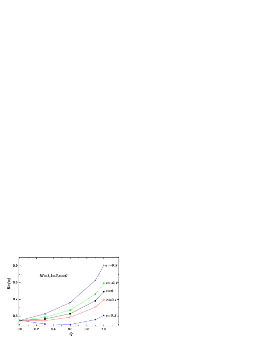
Figure 3: Real part of Quasinormal frequencies of $e=0$, $\pm 0.1$, $\pm 0.3$ with $Q$ at $M=1$, $l=3$, $n=0$.

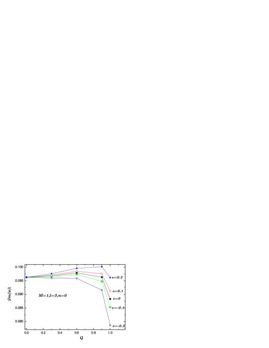
Figure 4: Absolute value of imaginary part of Quasinormal frequencies of $e=0$, $\pm 0.1$, $\pm 0.3$ with $Q$ at $M=1$, $l=3$, $n=0$.

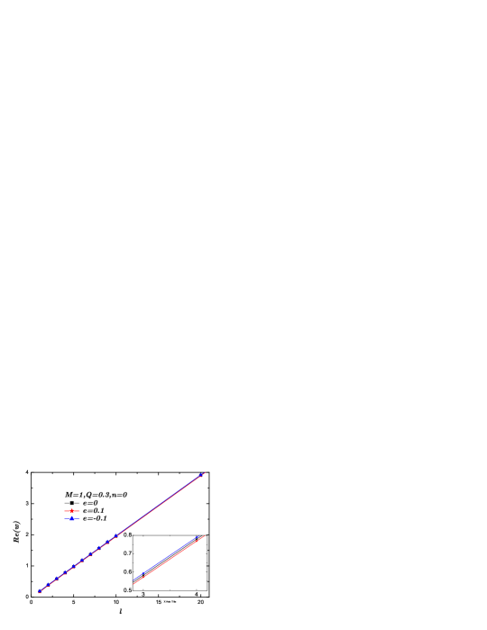
Figure 5: Real part of Quasinormal frequencies of $e=0$, $\pm 0.1$ with $l$ at $M=1$, $Q=0.3$, $n=0$.

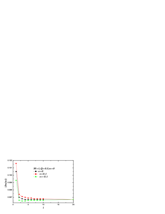
Figure 6: Absolute value of imaginary part of Quasinormal frequencies of $e=0$, $\pm 0.1$ with $l$ at $M=1$, $Q=0.3$, $n=0$.

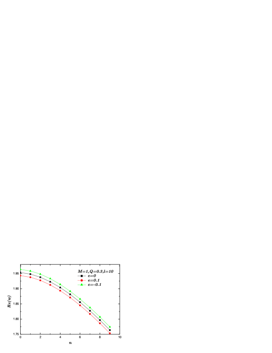
Figure 7: Real part of Quasinormal frequencies of $e=0$, $\pm 0.1$ with $n$ at $M=1$, $Q=0.3$, $l=10$.

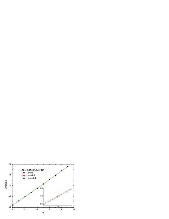
Figure 8: Absolute value of imaginary part of Quasinormal frequencies of $e=0$, $\pm 0.1$ with $n$ at $M=1$, $Q=0.3$, $l=10$.

Table 1: The quasinirmal frequencies for RN black hole, $l=3$, $4$, $5$, $n=0$, $e=0$, $\pm 0.1$, $\pm 0.3$, $M=1$, $Q=0$, $0.3$, $0.6$, $0.9$, $0.99$.

$l$	$n$	$e$	$Q=0.3$		$Q=0.6$		$Q=0.9$		$Q=0.99$
			$Re(w)$	$Im(w)$	$Re(w)$	$Im(w)$	$Re(w)$	$Im(w)$	$Re(w)$	$Im(w)$
1	0	0.1	0.1701	-0.1016	0.1712	-0.1034	0.1835	-0.1018	0.1879	-0.0982
		0	0.1799	-0.1005	0.1919	-0.1012	0.2207	-0.0979	0.2336	-0.0902
		-0.1	0.1900	-0.0993	0.2138	-0.0987	0.2610	-0.0929	0.2849	-0.0808
2	0	0.1	0.3746	-0.0974	0.3844	-0.0990	0.4197	-0.0984	0.4418	-0.0936
		0	0.3847	-0.0970	0.4059	-0.0981	0.4581	-0.0963	0.4891	-0.0898
		-0.1	0.3949	-0.0966	0.4279	-0.0972	0.4978	-0.0941	0.5387	-0.0856
	1	0.1	0.3499	-0.3016	0.3614	-0.3059	0.4008	-0.3017	0.4205	-0.2863
		0	0.3602	-0.2999	0.3834	-0.3023	0.4396	-0.2944	0.4668	-0.2740
		-0.1	0.3706	-0.2982	0.4057	-0.2987	0.4795	-0.2868	0.5152	-0.2609
3	0	0.1	0.5726	-0.0971	0.5923	-0.0985	0.6528	-0.0976	0.6912	-0.0924
		0	0.5827	-0.0968	0.6140	-0.0979	0.6915	-0.0963	0.7390	-0.0899
		-0.1	0.5929	-0.9651	0.6360	-0.0973	0.7311	-0.0948	0.7882	-0.0872
	1	0.1	0.5552	-0.2953	0.5762	-0.2994	0.6397	-0.2959	0.6716	-0.2799
		0	0.5655	-0.2943	0.5982	-0.2973	0.6787	-0.2913	0.7242	-0.2715
		-0.1	0.5759	-0.2933	0.6204	-0.2952	0.7185	-0.2865	0.7730	-0.2632
	2	0.1	0.5268	-0.5010	0.5498	-0.5076	0.6178	-0.4997	0.6454	-0.4802
		0	0.5372	-0.4992	0.5719	-0.5037	0.6566	-0.4914	0.6971	-0.4578
		-0.1	0.5476	-0.4974	0.5942	-0.4997	0.6962	-0.4830	0.7445	-0.4436

Table 2: The quasinirmal frequencies for RN black hole, $l=3$, $4$, $5$, $n=0$, $e=0$, $\pm 0.1$, $\pm 0.3$, $M=1$, $Q=0$, $0.3$, $0.6$, $0.9$.

$l$	$e$	$Q=0$		$Q=0.3$		$Q=0.6$		$Q=0.9$
		$Re(w)$	$Im(w)$	$Re(w)$	$Im(w)$	$Re(w)$	$Im(w)$	$Re(w)$	$Im(w)$
3	0.3			0.5525	-0.0976	0.5498	-0.0996	0.5783	-0.1002
	0.1			0.5726	-0.0971	0.5923	-0.0985	0.6528	-0.0976
	0	0.5737	-0.0963	0.5827	-0.0968	0.6140	-0.0979	0.6915	-0.0963
	-0.1			0.5929	-0.0965	0.6360	-0.0973	0.7311	-0.0948
	-0.3			0.6135	-0.0960	0.6808	-0.0959	0.8130	-0.0916
4	0.3			0.7488	-0.0976	0.7561	-0.0992	0.8095	-0.0994
	0.1			0.7690	-0.0970	0.7991	-0.0983	0.8850	-0.0974
	0	0.7672	-0.0963	0.7792	-0.0967	0.8208	-0.0979	0.9239	-0.0963
	-0.1			0.7894	-0.0965	0.8428	-0.0974	0.9634	-0.0952
	-0.3			0.8099	-0.0961	0.8873	-0.0964	1.0444	-0.0928
5	0.3			0.9448	-0.0972	0.9623	-0.0990	1.0408	-0.0988
	0.1			0.9650	-0.0969	1.0053	-0.0982	1.1169	-0.0972
	0	0.9602	-0.0963	0.9752	-0.0967	1.0272	-0.0979	1.1559	-0.0963
	-0.1			0.9854	-0.0966	1.0491	-0.0975	1.1953	-0.0954
	-0.3			1.0059	-0.0962	1.0936	-0.0967	1.2759	-0.0935

Table 3: The quasinirmal frequencies for RN black hole, $l=1$, …, $5$, $10$, $20$, $n=0$, $Q=0.3$, $e=0$, $\pm 0.1$.

	$e$	$l=1$	$l=2$	$l=3$	$l=4$	$l=5$	$l=10$	$l=20$
$Re(w)$	0	0.1799	0.3847	0.5827	0.7792	0.9752	1.9534	3.9082
	0.1	0.1701	0.3746	0.5726	0.7690	0.9650	1.9432	3.8980
	-0.1	0.1900	0.3949	0.5929	0.7894	0.9854	1.9636	3.9184
$Im(w)$	0	-0.1005	-0.0970	-0.0968	-0.0967	-0.0967	-0.0967	-0.0967
	0.1	-0.1016	-0.0974	-0.0971	-0.0970	-0.0969	-0.0968	-0.0967
	-0.1	-0.0993	-0.0966	-0.9651	-0.0965	-0.0966	-0.0966	-0.0967

Table 4: The quasinirmal frequencies for RN black hole, $n=0,...,7$, $l=8$, $Q=0.3$, $e=0$, $\pm 0.1$.

	$e$	$n=0$	$n=1$	$n=2$	$n=3$	$n=4$	$n=5$	$n=6$	$n=7$
$Re(w)$	0	1.9534	1.9481	1.9379	1.9230	1.9040	1.8815	1.8558	1.8257
	0.1	1.9432	1.9379	1.9276	1.9127	1.8937	1.8711	1.8454	1.8171
	-0.1	1.9636	1.9584	1.9481	1.9333	1.9144	1.8918	1.8662	1.8379
$Im(w)$	0	-0.0967	-0.2904	-0.4852	-0.6814	-0.8794	-1.0795	-1.2814	-1.4852
	0.1	-0.0968	-0.2907	-0.4856	-0.6820	-0.8803	-1.0806	-1.2827	-1.4867
	-0.1	-0.0966	-0.2902	-0.4847	-0.6807	-0.8786	-1.0784	-1.2801	-1.4837