Possibilities for Measurement and Compensation of Stray DC Electric Fields Acting on Drag-Free Test Masses

Abstract

DC electric fields can combine with test mass charging and thermal dielectric voltage noise to create significant force noise acting on the drag-free test masses in the LISA (Laser Interferometer Space Antenna) gravitational wave mission. This paper proposes a simple technique to measure and compensate average stray DC potentials at the mV level, yielding substantial reduction in this source of force noise. We discuss the attainable resolution for both flight and ground based experiments.

1 INTRODUCTION

In the envisioned design of the gravitational wave mission LISA, capacitive sensors will provide the readout of the relative position of the satellites with respect to the freely flying test masses, which serve both as interferometry end mirrors and drag-free orbit references (Bender, 2000). A drawback of electrostatic sensors is that the combined needs of high precision ($\approx$ nm$/\sqrt{\mathrm{Hz}}$) and low electrostatic force gradients require a small distance (or gap, $d$) between the test mass and sensing electrodes. This need for proximity, introduces a number of less easily characterized short range force effects, electrostatic and otherwise, which grow with decreasing gap and can dominate the low frequency test mass acceleration noise. An important example is DC electric fields, which produce both force gradients (or “stiffness”) increasing as $d^{-3}$ and, coupled with charging and dielectric noise, force noise proportional to, respectively, $d^{-1}$ and $d^{-3/2}$. Though the current sensor design for the European LISA demonstrator flight experiment LTP (Vitale, 2002), calls for relatively large 4 mm gaps along the sensitive x axis in order to limit these short range effects (Weber, 2002), DC fields are still expected to be a significant noise source.

Stray DC fields, related to spatially varying DC surface potentials known as patch fields, can arise from the different work function of domains exposing different crystalline facets. These fields statistically average over the small grains, which for gold surfaces can be micron size and produce RMS surface potential variations of order 1 mV on mm length scales (Camp, 1992). These are not likely to be a significant problem for the designed sensor, shown schematically in Fig. 1, where 4 mm x axis gaps provide distance for the fields and gradients to fall off, as well as an effective dilution of the smaller length scale variations (Speake, 1996). Potentially more dangerous are patch fields with relatively large coherence lengths, caused by surface contamination from the assembly and from material outgassing over a long mission. Noise models have assumed typical average whole electrode DC biases $\delta V$ of order 100 mV (Weber, 2002).

Electrostatic actuation circuitry, to be integrated with the sensor for application of forces using audio frequency modulated voltages, will also allow direct application of DC voltages to the sensing electrodes. We analyze here, as a way to reduce the total acceleration noise caused by stray DC biases, the use of applied actuation voltages to first measure the average biases and then compensate to make the average DC potential zero. The electrostatic model considered here considers each electrode electrode at a single potential, without spatial variation. This much simplified analysis addresses what we can actually change with a single applied voltage per electrode, the average DC potential. This approach is still relevant, as the likely dominant effect, the interaction of DC fields with the noisy test mass charge, is realistically parametrized, and thus curable, by the average DC potential on the electrodes. We start with a description of the noise sources related to stray DC biases, then turn to the techniques for measuring and balancing them, both in flight and on the ground.

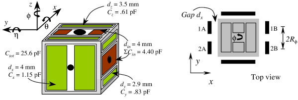
Fig. 1: Schematic of proposed capacitive sensor, with capacitance and gap values, adapted from Weber (2002). The injection electrodes used to provide the sensing bias are darkly shaded, the sensing electrodes are medium gray, and grounded guard ring surfaces are light gray. The planned test mass is a 46 mm, 2 kg Au / Pt cube.

2 NATURE OF THE PROBLEM: NOISY FORCES ARISING FROM DC FIELDS

We analyze here the simplified model of the sensor in Fig. 2. Four x sensing electrodes, opposing pairs 1A/1B and 2A/2B, face the test mass along the x axis. Functionally, differential measurements of the two capacitor pairs are combined to yield the test mass x translational and $\phi$ rotational displacements (Weber, 2002). Assigning electrode potentials $V_{j}$ and an accumulated test mass charge $q$, the instantaneous x force component $F_{x}$ and test mass potential $V_{M}$ can be expressed

$$F_{x} = \frac{1}{2}\sum_{i}{\frac{\partial C_{i}}{\partial{x}}\left(V_{i}-V_{M}\right)^{2}}$$ (1)

$$V_{M} = \frac{q}{C_{T}}+\frac{1}{C_{T}}\sum_{j}{C_{j}V_{j}}$$ (2)

$C_{T}$ is the total capacitance of the test mass to all other surfaces. We sum here over all sensor conducting surfaces, $i$, but also note that $\frac{\partial C_{i}}{\partial{x}}$ will have non-zero contributions only from the 4 x sensing electrodes and, when the mass is translated off center in x, from grounded guard ring surfaces (see Fig. 1).

While the x electrodes will nominally be held at DC ground by the sensing / actuation circuitry (Weber, 2002), we consider here for each a non-zero $V_{i}$ caused by the sum of a stray DC bias $\delta V_{i}$ and a thermal noise voltage $v_{ni}$ (later, we will consider the possibility of compensating $\delta V_{i}$ with an added applied DC bias, $V_{ai}$). Noisy low frequency forces along x arise in the interaction between $\delta V_{i}$ and low frequency fluctuations in $q$ and $v_{ni}$. The charge $q$ accumulated from cosmic ray events evolves in a random walk process, with an estimated effective step rate of $\lambda_{eff}\approx 260$ $e$/s (Araújo, 2002), producing a “red” charge spectral density $S_{Q}^{1/2}=\frac{e}{\omega}\sqrt{2\lambda_{eff}}$. The thermal noise $v_{ni}$, originating in lossy dielectric layers on the electrode and test mass surfaces, is characterized by loss angle, $\delta$, assumed here to be of order 10^-5 for Au coated surfaces (Speake, 1999), with spectral density $S_{v_{n}}^{1/2}=\sqrt{4k_{B}T\frac{\delta}{\omega C_{x}}}$.

In evaluating Eqns. 1 and 2 for the force disturbance, we define the nominal (test mass centered) capacitances and first derivatives, $C_{x}$ and $\pm\frac{C_{x}}{d_{x}}$ (neglecting edge effects, $d_{x}$ is the electrode - test mass gap). Substituting $\delta V_{i}$, $q$, and $v_{ni}$ into Eq. 1, we evaluate the leading order force, and resulting acceleration noise spectral density $S_{a}^{1/2}$, caused by the charge noise:

$$F_{x} \approx -\frac{q}{C_{T}}\frac{C_{x}}{d_{x}}\Delta_{x}$$ (3)

$$S_{a_{charge}}^{1/2} \approx 7\times 10^{-15}\>\mathrm{m/s^{2}/\sqrt{Hz}}\times\left(\frac{\Delta_{x}}{\sqrt{4}\times 100\>\mathrm{mV}}\right)\left(\frac{\lambda_{eff}}{260\>\mathrm{/s}}\right)^{1/2}\left(\frac{0.1\>\mathrm{mHz}}{f}\right)\>\>\>,$$ (4)

where we define $\Delta_{x}\equiv\left(\delta V_{1B}+\delta V_{2B}-\delta V_{1A}-\delta V_{2A}\right)$. For the dielectric loss noise:

$$F_{x} \approx \sum_{i}{\frac{\partial C_{i}}{\partial{x}}v_{ni}\left(\delta V_{i}-\frac{q}{C_{T}}-\frac{1}{C_{T}}\sum_{j}{\delta V_{j}C_{j}}\right)}$$ (5)

$$S_{a_{diel}}^{1/2} \approx 5\times 10^{-16}\>\mathrm{m/s^{2}/\sqrt{Hz}}\times\left(\frac{\delta V}{100\>\mathrm{mV}}\right)\left(\frac{\delta}{10^{-5}}\right)^{1/2}\left(\frac{0.1\>\mathrm{mHz}}{f}\right)^{1/2}$$ (6)

To estimate a number for $S_{a_{diel}}^{1/2}$, we use $q=\sum_{j}{C_{j}\delta V_{j}}=0$.

The random charging produces a coherent disturbance multiplied by the average difference of DC potential seen on either side of the test mass, $\Delta_{x}$. This is true, neglecting edge effects, independently of the details of the surface potential distribution. On the other hand, no such averaging occurs in the “beating” of the DC voltages against the dielectric loss thermal noise, which will be uncorrelated between electrodes.

The acceleration noise target for LISA is $3\times 10^{-15}$ m/s²$/\sqrt{\mathrm{Hz}}$, so the random charge noise in Eq. 4 is potentially performance-spoiling at .1 mHz, the nominal low end of the LISA measurement band and has an increasingly dominant effect with decreasing frequency, where there is growing scientific interest to extend the gravitational wave measurement band (Bender, 2002). The dielectric loss effect looks less threatening, but is difficult to estimate of the contamination dependence of the loss angle $\delta$. With DC voltages thus problematic at the 100 mV level, the effects described in Eqns. 4 and 6 illustrate the importance of AC carrier voltages, rather than DC, in applying the necessary DC and low frequency actuation forces, which demand RMS levels of several volts (Weber, 2002).

3 MEASUREMENT OF DC BIASES

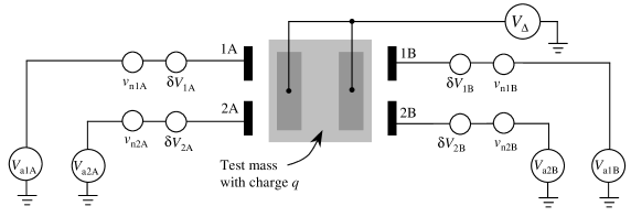
Fig. 2: Schematic of the simplified, four electrode electrostatic model and measurement technique analyzed here. Stray DC biases, dielectric noise, and test mass charge are denoted $\delta V_{i}$, $v_{ni}$, and $q$. In the main measurement described in the text, a modulated bias $V_{\Delta}$ is applied to the test mass via the z electrodes. Actuation voltages $V_{ai}$ can be applied to compensate the $\delta V_{i}$ and can also modulate the electrode voltages in other measurements.

There are a number of ways to measure the stray DC electrode biases. Here we present one measurement in detail, illustrated in Fig. 2 and (a) in Fig. 3, and mention several other, (b)-(e) in Fig. 3. In configuration (a), a sinusoidal signal $V_{\Delta}\sin{\omega_{0}t}$ applied to the four z sensing electrodes makes the test mass potential oscillate with amplitude $\frac{4C_{z}}{C_{T}}V_{\Delta}\equiv\alpha V_{\Delta}$ ($\alpha\approx.1$ for the sensor design in Fig. 1). The modulating test mass bias simulates, from the standpoint of forces in the $xy$-plane, an oscillating test mass charge.

In expanding Eqns. 1 and 2 to first order in displacement for the force $F_{x}$ (and an analogous equation for the torque $N_{\phi}$), we make use of the second derivative $\frac{\partial^{2}C_{x}}{\partial{x}^{2}}\approx+\frac{2C_{x}}{d_{x}^{2}}$, as well as the derivatives involving the mass rotation $\phi$, $\frac{\partial C_{x}}{\partial{\phi}}\equiv\pm C_{x}\frac{R_{\phi}}{d_{x}}$, $\frac{\partial^{2}C_{x}}{\partial{\phi}^{2}}\equiv+\frac{2C_{x}R_{2\phi}^{2}}{d_{x}^{2}}$, and $\frac{\partial^{2}C_{x}}{\partial x\partial\phi}\equiv\pm\frac{2C_{x}R_{\phi}}{d_{x}^{2}}$ ($R_{\phi}$ is half the on-center electrode separation, neglecting edge effects, and $R_{2\phi}$ has roughly the same magnitude). The force and torque produced at the first and second harmonic of the voltage modulation frequency $\omega_{0}$ are given by

$$F_{1\omega_{0}} = \alpha V_{\Delta}\>\sin{\omega_{0}t}\>\left\{-\Delta_{x}\frac{C_{x}}{d_{x}}\>+\>\left[\left(4V_{M0}-\Sigma_{x}\right)\frac{2C_{x}}{d_{x}^{2}}+V_{M0}\frac{\partial^{2}C_{g}}{\partial{x}^{2}}\right]x\>-\>\frac{2C_{x}R_{\phi}}{d_{x}^{2}}\Delta_{12}\>\phi\right\}$$ (7)

$$F_{2\omega_{0}} = -\alpha^{2}V_{\Delta}^{2}\cos{2\omega_{0}t}\left(\frac{2C_{x}}{d_{x}^{2}}+\frac{1}{4}\frac{\partial^{2}C_{g}}{\partial{x}^{2}}\right)\>x\>$$ (8)

$$N_{1\omega_{0}} = \alpha V_{\Delta}\>\sin{\omega_{0}t}\>\left\{-\Delta_{\phi}\frac{C_{x}R_{\phi}}{d_{x}}\>+\>\left[\left(4V_{M0}-\Sigma_{x}\right)\frac{2C_{x}R_{2\phi}^{2}}{d_{x}^{2}}+V_{M0}\frac{\partial^{2}C_{g}}{\partial{\phi}^{2}}\right]\phi\>-\>\Delta_{12}\frac{2C_{x}}{d_{x}}\>x\right\}$$ (9)

$$N_{2\omega_{0}} = -\alpha^{2}V_{\Delta}^{2}\cos{2\omega_{0}t}\>\left(\frac{2C_{x}R_{2\phi}^{2}}{d_{x}^{2}}+\frac{1}{4}\frac{\partial^{2}C_{g}}{\partial{\phi}^{2}}\right)\>\phi\>$$ (10)

For convenience we have defined the combined stray DC biases $\Delta_{\phi}\equiv\left(\delta V_{1A}+\delta V_{2B}-\delta V_{2A}-\delta V_{1B}\right)$,$\Delta_{12}\equiv\left(\delta V_{2A}+\delta V_{2B}-\delta V_{1A}-\delta V_{1B}\right)$, and $\Sigma_{x}\equiv\left(\delta V_{1A}+\delta V_{1B}+\delta V_{2A}+\delta V_{2B}\right)$. We also make use of the test mass potential when centered in the absence of any applied fields, $V_{M0}\equiv\frac{q}{C_{T}}+\frac{\sum_{j}{\delta V_{j}C_{j0}}}{C_{T}}$.

The 2$\omega_{0}$ terms, in Eqns. 8 and 10 are pure “stiffness,” or position dependent, terms related only to the applied bias. The test mass can be positioned to make the 2$\omega_{0}$ force signal disappear, which centers the mass to then eliminate the stiffness terms in the 1$\omega_{0}$ force and torque terms, making the measurement independent of $V_{M0}$ (and charge). The self-calibrating location of the “force zero” with the 2$\omega_{0}$ force signals is useful because the force zero (roughly speaking, where the capacitance derivatives are equal) will not, due to machining imperfections and asymmetries, coincide exactly with the sensor readout zero, where the capacitances themselves are equal. With the test mass centered, the remaining x force is thus a 1$\omega_{0}$ signal cleanly proportional to the differential bias $\Delta_{x}$ of relevance to the random charging force noise. Likewise, a null measurement test is possible after compensation voltages are applied.

In principle, the forces and torques detectable in Eqns. 7 - 10 offer all the information measurable for the average electrode DC biases and test mass charge. $\Delta_{x}$ and $\Delta_{\phi}$ are the main 1$\omega_{0}$ signals in force and torque, with $\Delta_{12}$ and $\left(\Sigma_{x}-4V_{M0}\right)$ entering in the stiffness and thus measurable in the position dependence of the signals. These quantities can, however, be measured better individually, with the test mass centered, using opportune modulation of the channel 1 and 2 actuation voltages. Four symmetric schemes, which permit the 2$\omega_{0}$ centering procedure and together give a complete average DC bias characterization by measurement of the 1$\omega_{0}$ force terms, are illustrated schematically in Fig. 3 (b) - (e).

It is worthwhile commenting here on the applicability of this simplified model, given the realistic spatial fluctuations present in electrode surface potentials. If we considered x electrodes divided into many surface domains, each with a different bias $\delta V_{i}$ but all still a distance $d_{x}$ from the test mass, and apply the configuration (a) $V_{\Delta}$ bias, the centering process with the 2$\omega_{0}$ signal would be unchanged and, neglecting edge effects, the resulting 1$\omega_{0}$ force would still give the average potential difference $\Delta_{x}$. If we also included variations in the “grounded” guard ring potential, the effective average potential $\Delta_{x}$ relevant to the detected force would then also average over the guard rings stray bias distribution. Importantly, however, the applied biases $V_{ai}$ that null the force signal in this measurement will also null the effect of random charge on the test mass, including all stray DC fields biases generated inside (and even outside) the sensor.

The torques do not generalize as easily from the simple “one voltage per electrode” picture to spatially variable potentials, because the average potential of relevance to the torques is weighted by an effective arm length, or distance from the rotation axis. Thus, to balance the average electrode potentials relevant to the x force noise, the additional differential bias potentials are best measured by the x forces excited by the bias configurations in Fig. 3. The configurations using the x electrodes themselves for biasing are sensitive to the biases on those electrodes, much less so to any guard ring patch effects. Combining the measured $\Delta_{x}$, $\Delta_{\phi}$, $\Delta_{12}$, and $\left(4V_{M0}-\Sigma_{x}\right)$ allows calculation of the potentials $V_{ai}$ needed to null the detected forces and thus to bring all four sensing electrodes near to the test mass potential.

This procedure can be repeated for electrodes on the y and z faces. We finally note that the charge measurement configurations, such as (c) in Fig. 3, measure not just the charge but $\left(4V_{M0}-\Sigma_{x}\right)$ and thus will depend quantitatively on how well the surrounding DC biases are balanced.

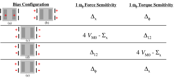
Fig. 3: Cartoon illustrating different electrode bias configurations useful in measurement of stray DC biases and charge, with the specific DC bias combinations producing 1$\omega_{0}$ forces and torques listed on the right. The + and - signs correspond to the relative phase of the modulated voltage applied to a given electrode.

4 IN-FLIGHT DETECTION AND BALANCING

In flight, the forces and torques described above can be detected by the position sensor signal itself. Both on LISA and LTP, a low frequency electrostatic suspension mode will be used to control the test mass non-drag-free degrees of freedom, and can also be applied on the sensitive x axis to make this measurement (Bortoluzzi, 2002). The suspension will have high gain at low frequencies to counteract DC forces and very low gain in the measurement band, such that, for forces applied at mHz frequencies, the test mass dynamics is roughly that of a free particle, with displacement $x\approx\frac{-f}{m\omega^{2}}$. For a 1 mHz modulation of $V_{\Delta}=1V$ (and thus roughly 100 mV test mass bias amplitude), the displacement would be of order 40 nm if $\Delta_{x}$ $\approx$ 100 mV.

The measurement resolution will likely be dominated by sensor noise and residual spacecraft motion, rather than the force noise acting on the test mass. For the LTP experiment, the goal for this total position noise is 5 nm$/\sqrt{\mathrm{Hz}}$(Bortoluzzi, 2002). The resulting resolution of $\Delta_{x}$ in integration time $T$ is then

$$\Delta\left(\Delta_{x}\right)\approx\frac{1}{\left|\frac{\partial F}{\partial\Delta_{x}}\right|}\frac{\sqrt{2}m\omega^{2}_{0}S_{{\it x}_{n}}^{1/2}}{\sqrt{T}}\approx 350\,\mathrm{\mu V}\>\times\left(\frac{1\,\mathrm{hr}}{T}\right)^{1/2}\left(\frac{1\,\mathrm{V}}{V_{\Delta}}\right)\left(\frac{S_{{\it x}_{n}}^{1/2}}{5\,\mathrm{nm/Hz^{1/2}}}\right)\left(\frac{\omega_{0}}{2\pi\times 1\,\mathrm{mHz}}\right)^{2}$$ (11)

A one hour experiment could thus allow sub-mV resolution of the stray DC bias difference $\Delta_{x}$. The resolution limit in the balancing of the applied biases will be limited, for LTP, to the 1 mV level by the envisioned 16 bit, $\pm$ 40 V full scale actuation DA converter and amplifier (Vitale, 2002). Any instability in the balancing voltage will multiply this residual mV level voltage to produce a noisy force, but the projected actuation voltage stability, of order $10^{-6}$$/\sqrt{\mathrm{Hz}}$, makes this a neglible source of force noise (Vitale, 2002). Note that balancing of $\Delta_{x}$ to the mV level would reduce the acceleration noise caused by random charging below the .1 fm/s²$/\sqrt{\mathrm{Hz}}$ level at .1 mHz, and thus well below the LISA target acceleration noise.

5 TORSION PENDULUM GROUND TESTING

Current ground based measurement programs will use torsion pendulums to characterize weak forces and force gradients of relevance to drag-free control (Hueller, 2002). Suspending a test mass as the pendulum inertial member, surrounded by a LISA or LTP prototype sensor, permits sensitive, high isolation, low restoring force measurements for a single torsional degree of freedom. A pendulum comprised of a single test mass suspended on axis with the torsion fiber is sensitive to torques, while a pendulum with a test mass held off the rotation axis will convert translational forces into measurable pendulum angular deflections.

With the single mass configuration, the rotational DC bias imbalance $\Delta_{\phi}$ can be measured using a z electrode bias $V_{\Delta}$, with the torque (see Eq. 9) detected in the pendulum deflection. The measurement resolution will likely be limited by the mechanical torque noise acting on the pendulum, $S_{N}^{1/2}$,

$$\Delta\left(\Delta_{\phi}\right)\approx\frac{1}{\left|\frac{\partial N}{\partial\Delta_{\phi}}\right|}\frac{\sqrt{2}S_{N}^{1/2}}{\sqrt{T}}\approx 400\,\mathrm{\mu V}\>\times\left(\frac{1\,\mathrm{hr}}{T}\right)^{1/2}\left(\frac{1\,\mathrm{V}}{V_{\Delta}}\right)\left(\frac{S_{N_{n}}^{1/2}}{5\,\mathrm{fN\,m/Hz^{1/2}}}\right)$$ (12)

Here, 5 fN m$/\sqrt{\mathrm{Hz}}$ refers to the expected 1 mHz thermal torque noise limit for the designed one mass pendulum (Hueller, 2002). Higher torque noise would necessitate an increased $V_{\Delta}$ to maintain this resolution.

The torsion pendulum measurement has several possible systematic errors. Because the pendulum is relatively insensitive to purely translational forces, there will not be a 2$\omega_{0}$ force signal to center in x. Centering in x will thus depend on the sensor translational readout zero, which could differ from the force zero by order 10 $\mu$m, set by the sensor machining tolerances (Vitale, 2002). The offset in x means the x stiffness term in Eq. 9 will not vanish, producing, for $\left|\Delta_{12}\right|\approx$ 200 mV, a systematic error of roughly 1 mV in the measurement of $\Delta_{\phi}$. Another error enters in the finite “twist-tilt” feedthrough (Smith, 1999) that can couple the electrostatic force, proportional to $\Delta_{x}$, into the measured torsional rotation. However, assuming that $\Delta_{\phi}$ and $\Delta_{x}$ are of the same order of magnitude, the ratio between the excited pendulum swing angle and the torsional twist angle will be of order 10^-6, giving an immeasurably small effect for typical values of twist-tilt coupling. Thus, measurement and balancing of $\Delta_{\phi}$ looks feasible at the mV level with the torsion pendulum and could provide a valuable ground test of the compensation technique suggested here.

6 CONCLUSION

The true magnitude and long term stability of the stray DC potentials for LISA will not be known until the actual flight experiment begins. However, the average fields are measurable and can be balanced. Compensating the average stray electrode biases should be quite effective in cancelling a potentially large random charging noise source, where balancing the average potential seen on either side of the test mass should null the force from a deposited charge. For the lossy dielectric noise, however, which itself could be spatially dependent, the average potential alone may not adequately characterize the phenomena, and the success of the compensation in reducing this source of acceleration noise will depend on the extent to which the thermal noise causes the “patches” across an entire electrode to fluctuate in unison.

7 ACKNOWLEDGEMENTS

The authors would like to acknowledge Peter Bender for bringing the the random charging problem, and its possible compensation, to our attention.

8

Corresponding author: W. J. Weber, weber@science.unitn.it

References

- [1] P. Bender et al., LISA: A Cornerstone Mission for the Observation of Gravitational Waves, ESA-SCI(2000)11 System and Technology Study, 2000.
- [2]
- [3] Vitale, S., LISA Technology Package Architect Final Report ESTEC contract #15580/01/NL/HB, 2002.
- [4]
- [5] Weber, W. J., D. Bortoluzzi, A. Cavalleri et al., Position Sensors for Flight Testing LISA Drag-free Control, submitted to Proc. SPIE Astronomical Telescopes and Instrumentation Conference, 2002.
- [6]
- [7] Camp, J. B., T. W. Darling, and R. E. Brown, Effect of Crystallites on Surface Potential Variations of Au and Graphite, J. Appl. Phys 71 783-85, 1992.
- [8]
- [9] Speake, C. C., Forces and Force Gradients Due to Patch Fields and Contact Potential Differences, Class. Quantum Grav., 13 A291-297, 1996.
- [10]
- [11] Araújo H. M., A. Howard, D. Davidge et al., Charging of Isolated Proof Masses in Satellite Experiments such as LISA, submitted to Proc. SPIE Astronomical Telescopes and Instrumentation Conference, 2002.
- [12]
- [13] Speake, C. C., R. S. Davis, T. J. Quinn et al., Electrostatic Damping and its effect on Precision Mechanical Experiments, Phys. Lett A, 263 219-225, 1999.
- [14]
- [15] Bender, P. L., LISA Sensitivity Below 0.1 Millihertz, submitted to Class. Quantum Grav, 2002.
- [16]
- [17] Bortoluzzi, D., P. Bosetti, L. Carbone et al., Testing LISA Drag-free Control Technology with the LISA Technology Package Flight Experiment, submitted to Class. Quantum Grav, 2002.
- [18]
- [19] Hueller, M., A. Cavalleri, R. Dolesi et al., Torsion Pendulum Facility for Ground Testing of Gravitational Sensors for LISA, Class. Quantum Grav., 19 1757-1765, 2002.
- [20]
- [21] Smith, G. I., C. D. Hoyle, J. H. Gundlach et al., Short-range Tests of the Equivalence Principle, Phys. Rev. D 61 022001-20, 1999.
- [22]
8