Kinematical bound in asymptotically translationally invariant spacetimes

Abstract

We present positive energy theorems in asymptotically translationally invariant spacetimes which can be applicable to black strings and charged branes. We also address the bound property of the tension and charge of branes.

I Introduction

Asymptotic flatness is a useful working assumption in studying four-dimensional general relativity, in particular in the field of the black hole physics. Of course, this assumption is well justified for the gravitational phenomena of isolated systems within the Hubble horizon of our universe. Within the framework of the string theory, on the other hand, we have to take account of non-asymptotically flat space-times, because the vacuum of the theory is considered to be four-dimensional space-time times compact extra dimensions at low energy to realize our apparently four-dimensional universe. For example, we need more insight into the black strings of branes, which are non-asymptotically flat solutions typically arising in the supergravity theories, to extract some information on the quantum gravity or the unified theory of interactions.

The stability of the Schwarzschild space-time is one of fundamental properties of the black holes in asymptotically flat space-time. However, this is not the case for the black strings or branes; namely, they are unstable under the linear perturbations of sufficiently long wave length along the brane GL . We have no definitive answer concerning the end point of this Gregory-Laflamme instability, but there are several possibilities; the final state might be naked singularities joining array of black holes, or inhomogeneous black string or brane Gary , and there also be a possibility that there is no equilibrium state. Since the subject concerns with non-asymptotically flat inhomogeneous space-time, the analysis will be quite difficult. We would ultimately need dynamical analysis directly solving the Einstein equation BS ; Toby . It might be however also useful to have a kinematical bound irrelevant for the details of the underlying theory for such non-asymptotically flat space-times. Such a kinematical bound might be also useful to restrict the form of the metric like the uniqueness theorem in asymptotically flat spacetimes Israel ; UniqTheo1 .

In this short report, utilizing the spinorial approach, we present bound theorems (positive mass theorem, BPS bound, positive tension theorem) in asymptotically translationally invariant space-times. Recently Traschen discussed the positive mass theorem in such space-times without horizon and gauge fieldsJennie2 . In this paper we will extend the Traschen’s work to the cases with horizon in higher dimensions, which is relevant for black string or brane space-times, and include the gauge fields in four dimensions.

The rest of the present paper is composed of two main parts. In Sec. II, we present the positive mass theorem in higher dimensions with horizon. Then we prove the positive energy and tension theorems for charged branes in Sec. III. Finally we give a discussion in Sec. IV. In the appendix A we give formulae for the calculation of the boundary term at horizon.

II Asymptotically translationally invariant space-times

First of all, we must specify asymptotically translationally invariant space-times. The metric of full space-times is given by

$$ds^{2}=g_{\mu\nu}dx^{\mu}dx^{\nu}.$$ (1)

Let $n\propto\partial_{t}$ and $z\propto\partial_{x^{1}}$ to be timelike and spacelike unit vector fields such that $n^{\mu}z_{\mu}=0$. In addition, $\hat{r}\propto\partial_{x^{2}}$ to be spacelike perpendicular unit normal vector fields to $n$ and $z$, $\hat{r}^{\mu}n_{\mu}=\hat{r}^{\mu}z_{\mu}=0$. We assume that $z$ becomes to be proportional to asymptotically translational Killing vector toward the infinity directed to $\hat{r}$. $x^{\mu}$, $x^{i}$, $x^{I}$, $x^{A}$ and $x^{a}$ spans the full space-times ${\cal M}$, $(n-1)$-dimensional spacelike hypersurface $V_{0}$ normal to $n$, $(n-1)$-dimensional timelike hypersurface $V_{1}$ normal to $z$, $(n-2)$-dimensional spacelike submanifold $V_{01}$ orthogonal to $n$ and $z$, and $(n-3)$-dimensional spacelike submanifold $V_{012}$ orthogonal to $n$, $z$, $\hat{r}$. Each induced metricies can be written as

$$q_{ij}dx^{i}dx^{j}=(g_{\mu\nu}+n_{\mu}n_{\nu})dx^{\mu}dx^{\nu}$$ (2)

$$h_{IJ}dx^{I}dx^{J}=(g_{\mu\nu}-z_{\mu}z_{\nu})dx^{\mu}dx^{\nu}$$ (3)

$$p_{AB}dx^{A}dx^{B}=(g_{\mu\nu}+n_{\mu}n_{\nu}-z_{\mu}z_{\nu})dx^{\mu}dx^{\nu}$$ (4)

and

$$s_{ab}dx^{a}dx^{b}=(g_{\mu\nu}+n_{\mu}n_{\nu}-z_{\mu}z_{\nu}-\hat{r}_{\mu}\hat{r}_{\nu})dx^{\mu}dx^{\nu}.$$ (5)

Then $\mu,\nu=0,1,2,...,n$. $i=1,2,...,n$, $I=0,2,3,...,n$, $A=2,3,...n$, $a=3,4,...,n$. (See FIG.1.)

We assume that the submanifold $V_{01}$ is $(n-2)$-dimensional asymptotically Euclid space.

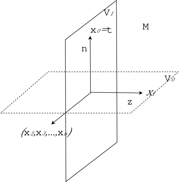
Figure 1: Full space-time $\cal{M}$ can be foliated by spacelike hypersurfaces $V_{0}$ normal to timelike vector field $n\propto\partial_{t}$ and timelike hypersurfaces $V_{1}$ normal to spacelike vector field $z\propto\partial_{x^{1}}$. We can define coordinate $\{x^{i}\}=(x_{1},x_{2},\cdots,x_{n})$ in $V_{0}$, $\{x^{I}\}=(x_{0},x_{2},\cdots,x_{n})$ in $V_{1}$ and $\{x^{A}\}=(x_{2},\cdots,x_{n})$ in $(n-2)-$dimensional spacelike surface $V_{01}$ normal to both vector fields $n$ and $z$. Furthermore, we set coordinate $\{x^{a}\}=(x_{3},\cdots,x_{n})$ in $(n-3)$-dimensional spacelike submanifold $V_{012}$ normal to $n,z$ and $\hat{r}\propto\partial_{x^{2}}$.

III Positive mass theorem for black string

In this section, we present the positive energy theorem in asymptotically translationally invariant space-time with horizon. See Ref. Jennie2 for cases without horizon. If one thinks of the gravitational energy evaluated in slices which has appropriate asymptotic boundaries and regular center, it is not necessary to take the event horizon as the boundary term. However, the proof independent of the inner structure of horizon is useful.

Let consider a spinor $\epsilon$ satisfying Dirac-type equationJennie2

$$\gamma^{A}\nabla_{A}\epsilon=0.$$ (6)

Note that we usually suppose $\gamma^{i}\nabla_{i}\epsilon=0$ for spinor to prove the original positive energy theoremPET . In asymptotically translationally invariant space-times, it is likely that the existence of solutions to Eq. (6), which approaches constant spinor $\epsilon_{0}$, is guaranteed rather than the solution to $\gamma^{i}\nabla_{i}\epsilon=0$. This is because the space spanned by coordinate $\{x^{A}\}$ is asymptotically flat and we can expect almost same proof of the existence of solutions with that in asymptotically flat space-times.

Let us define the Nester tensor $E_{\mu\nu}$ by

$$E^{\mu\nu}=\frac{1}{2}\biggl{(}\bar{\epsilon}\gamma^{\mu\nu\alpha}\nabla_{\alpha}\epsilon+{\rm c.c.}\biggr{)}$$ (7)

and we obtain formula

$$\nabla_{\mu}E^{\mu\nu}=\frac{1}{2}G^{\nu}_{\mu}\xi^{\mu}+{\overline{\nabla_{\mu}\epsilon}}\gamma^{\mu\nu\alpha}\nabla_{\alpha}\epsilon$$ (8)

where $\bar{\epsilon}=\epsilon^{\dagger}\gamma^{\hat{0}}$. According to Ref. PET , a surface integral of Nester tensor at spatial infinity over $V_{02}$ gives ADM energy-momentum vector $P^{\mu}$, that is,

$$-P^{\mu}\xi_{\mu}=\frac{1}{16\pi}\int_{V_{02}^{\infty}}E^{\mu\nu}dS_{\mu\nu}.$$ (9)

Integrating Eq.(8) over spacelike manifold $V_{02}$ and using Stokes’s theorem and Eq.(6), we obtain formula

$$\int_{V_{02}^{\infty}}dS_{\hat{0}\hat{2}}E^{\hat{0}\hat{2}}-\int_{V_{02}^{\rm H}}dS_{\hat{0}\hat{2}}E^{\hat{0}\hat{2}}$$

$$~{}~{}~{}~{}=\int dV_{0}\biggl{(}8\pi T^{\mu}_{\nu}\xi^{\nu}n_{\mu}+2|\nabla_{A}\epsilon|^{2}\biggr{)},$$ (10)

where $\xi^{\mu}=-\bar{\epsilon}\gamma^{\mu}\epsilon$. Following the proof in PET , we require a spinor $\epsilon$ approaches a constant spinor $\epsilon_{0}$ at infinity $V_{02}^{\infty}$. In the above we used the Einstein equation $G_{\mu\nu}=8\pi T_{\mu\nu}$. The first and second terms in the left-hand side are boundary terms at infinity and horizon. The first term gives us the gravitational energy. Thus, what we must focus on is the boundary term at the horizon. This is non-trivial issue and the point here. We modify the proof in asymptotically flat space-times with horizonBH . The detail of the computation is described in the appendix A. As a result, it becomes

$$\int_{V_{02}^{H}}dS_{\hat{0}\hat{2}}E^{\hat{0}\hat{2}} = \frac{1}{2}\int dS_{\hat{0}\hat{2}}\Biggl{[}\epsilon^{\dagger}(\nabla_{\hat{2}}-\gamma^{\hat{2}}\gamma^{\hat{1}}\nabla_{\hat{1}})\epsilon+{\rm c.c}\Biggr{]}$$ (11)

$$= \frac{1}{2}\int dS_{\hat{0}\hat{2}}\epsilon^{\dagger}\Biggl{[}-\frac{1}{2}(K-K_{\hat{2}\hat{2}}+k)\gamma^{\hat{2}}\gamma^{\hat{0}}\epsilon-\gamma^{\hat{2}}\gamma^{\hat{1}}D_{\hat{1}}\epsilon-\gamma^{\hat{2}}\gamma^{a}d_{a}\epsilon+\frac{1}{2}K_{\hat{a}\hat{2}}\gamma^{\hat{a}}\gamma^{\hat{0}}\epsilon\Biggr{]}+{\rm c.c.}$$

$$= \frac{1}{2}\int dS_{\hat{0}\hat{2}}\epsilon^{\dagger}\Biggl{[}-\frac{1}{2}(K-K_{\hat{2}\hat{2}}+k)\gamma^{\hat{2}}\gamma^{\hat{0}}\epsilon+\psi\Biggr{]}+{\rm c.c.}$$

where

$$\psi=-\gamma^{\hat{2}}\gamma^{\hat{1}}D_{\hat{1}}\epsilon-\gamma^{\hat{2}}\gamma^{a}d_{a}\epsilon+\frac{1}{2}K_{\hat{a}\hat{2}}\gamma^{\hat{a}}\gamma^{\hat{0}}\epsilon.$$ (12)

$D_{i},{\cal D}_{A}$ and $d_{a}$ are covariant derivative with respect to $q_{ij}$, $p_{AB}$ and $s_{ab}$, respectively. $K_{ij}$ and $k_{ab}$ are defined by $K_{ij}=q_{i}^{k}\nabla_{k}n_{j}$ and $k_{ab}=s_{a}^{c}{\cal D}_{c}\hat{r}_{b}$, respectively.

At the horizon we impose

$$\gamma^{\hat{2}}\gamma^{\hat{0}}\epsilon=\epsilon$$ (13)

and use $\theta_{+}\propto K-K_{\hat{2}\hat{2}}+k=0$ at the apparent horizon. $\theta_{+}$ is the expansion of outgoing null geodesic congruence. Then we can see the boundary term at the horizon vanishes. We used the fact that $\psi$ anti-commutes with $\gamma^{\hat{2}}\gamma^{\hat{0}}$ and then the contribution of $\psi$ to Eq. (11) disappears. Finally

$$E_{\rm ADM} = \frac{1}{8\pi|\epsilon_{0}|^{2}}\int_{V_{02}^{\infty}}dS_{\hat{0}\hat{2}}E^{\hat{0}\hat{2}}$$ (14)

$$= \frac{1}{8\pi|\epsilon_{0}|^{2}}\int dV_{0}\biggl{(}8\pi T^{\mu}_{\nu}\xi^{\nu}n_{\mu}+2|\nabla_{A}\epsilon|^{2}\biggr{)}.$$

Together with the dominant energy condition, we can see that $E_{\rm ADM}$ is positive definite.

Let us discuss $M=0$ cases. In this case,

$$\nabla_{\hat{A}}\epsilon=0$$ (15)

and then

$${}^{(n)}R_{\hat{A}\hat{B}\mu\nu}\gamma^{\mu\nu}\epsilon=0.$$ (16)

From the above we see

$${}^{(n)}R_{\mu\nu\alpha\beta}=0.$$ (17)

This means that the space-time with zero energy is flat. Even for asymptotically translationally invariant space-times, the ground state is flat space-time.

IV Bound theorems for charged branes in four dimensions

IV.1 Positive energy theorem for charged brane

In this subsection, we extend Traschen’s study to cases with gauge field in four dimensions. It is easy to extend to higher dimensions following Ref. GHT . For this we define the following covariant tensor motivated by N=2 supergravityN2PET :

$$\hat{\nabla}_{\mu}\epsilon=\nabla_{\mu}\epsilon+\frac{i}{4}F_{\alpha\beta}\gamma^{\alpha\beta}\gamma_{\mu}\epsilon.$$ (18)

Let us consider spinor $\epsilon$ satisfying

$$\gamma^{A}\hat{\nabla}_{A}\epsilon=0.$$ (19)

The Nester tensor is defined by

$$\hat{E}^{\mu\nu} = \frac{1}{2}\biggl{(}\bar{\epsilon}\gamma^{\mu\nu\alpha}\hat{\nabla}_{\alpha}\epsilon+{\bf c.c.}\biggr{)}$$ (20)

$$= E^{\mu\nu}-i\bar{\epsilon}(F^{\mu\nu}-\gamma_{5}\tilde{F}^{\mu\nu})\epsilon$$

and we obtain the following formula

$$\nabla_{\mu}\hat{E}^{\mu\nu} = \frac{1}{2}G^{\nu}_{~{}\mu}\xi^{\mu}+{\overline{\hat{\nabla}_{\mu}\epsilon}}\gamma^{\mu\nu\alpha}\hat{\nabla}_{\alpha}\epsilon$$ (21)

$$-i\bar{\epsilon}(\nabla_{\mu}F^{\mu\nu}-\gamma_{5}\nabla_{\nu}\tilde{F}^{\mu\nu})\epsilon$$

$$+4\pi\bar{\epsilon}T^{\mu\nu}(F)\gamma_{\nu}\epsilon$$

where $\tilde{F}^{\mu\nu}=(1/2)\epsilon^{\mu\nu\alpha\beta}F_{\alpha\beta}$ and

$$T_{\mu\nu}(F)=\frac{1}{4\pi}\Biggl{(}F_{\mu}^{~{}\alpha}F_{\nu\alpha}-\frac{1}{4}g_{\mu\nu}F^{2}\Biggr{)}.$$ (22)

Integrating over the spacelike hypersurface, we are resulted in

$$8\pi\epsilon^{\dagger}_{0}\Biggl{[}E_{\rm ADM}-i\gamma^{\hat{0}}(Q_{\rm e}-\gamma_{5}Q_{\rm m})\Biggr{]}\epsilon_{0} = \int_{V_{02}^{\infty}}dS_{\mu\nu}\hat{E}^{\mu\nu}$$ (23)

$$= \int_{V_{0}}d\Sigma\Biggl{[}G^{\mu}_{\nu}\xi^{\nu}n_{\mu}+2|\hat{\nabla}_{A}\epsilon|^{2}-2i\bar{\epsilon}(j^{\mu}_{\rm e}-\gamma_{5}j^{\mu}_{\rm m})\epsilon n_{\mu}-8\pi T_{\mu\nu}(F)\xi^{\mu}n^{\nu}\Biggr{]}$$

$$= \int_{V_{0}}d\Sigma\biggl{(}8\pi T^{\mu}_{\nu}\xi^{\nu}n_{\mu}+2|\hat{\nabla}_{A}\epsilon|^{2}-2i\bar{\epsilon}(j^{\mu}_{\rm e}-\gamma_{5}j^{\mu}_{\rm m})\epsilon n_{\mu}\biggr{)},$$

where

$$Q_{\rm e}=\frac{1}{8\pi}\int dS_{\mu\nu}F^{\mu\nu}$$ (24)

$$Q_{\rm m}=\frac{1}{8\pi}\int dS_{\mu\nu}\tilde{F}^{\mu\nu}$$ (25)

$$j^{\mu}_{\rm e}=\nabla_{\nu}F^{\nu\mu}$$ (26)

and

$$j^{\mu}_{\rm m}=\nabla_{\nu}\tilde{F}^{\nu\mu}.$$ (27)

From first line to second one, we used the Einstein equation $G_{\mu\nu}=8\pi(T_{\mu\nu}(F)+T_{\mu\nu})$. Using the above and the dominant energy condition, we can obtain the BPS bound

$$E_{\rm ADM}\geq{\sqrt{Q_{\rm e}^{2}+Q_{\rm m}^{2}}}.$$ (28)

As the inequality is saturated, $\hat{\nabla}_{\hat{A}}\epsilon=0$ holds. In general, $\hat{\nabla}_{\hat{0}}\epsilon\neq 0$ and $\hat{\nabla}_{\hat{1}}\epsilon\neq 0$. Since $\hat{\nabla}_{\hat{A}}\epsilon$ can be regarded as a infinitesimal local supersymmetric transformation of the gravitino, it is well-known fact that a part of supersymmetry is broken.

We note that the current BPS bound theorem is slightly different from that given in Ref. GHT .

IV.2 Positive tension theorem for charged branes

Let discuss the issue on the positive tension theoremJennie2 or BPS bound1st . As is discussed in Jennie2 , we can expect the tension of a brane is a conserved charge associated with an asymptotic spatial translational Killing vector parallel to the brane as ADM energy is one associated with an asymptotic time translational Killing vector. In analogy with the construction of positive energy theorem, the Nester tensor is defined by

$$\hat{B}^{\mu\nu} = \frac{1}{2}\biggl{(}\tilde{\epsilon}\gamma^{\mu\nu\alpha}\hat{\nabla}_{\alpha}\epsilon+{\rm c.c.}\biggr{)}$$ (29)

$$= \frac{1}{2}\biggl{(}\tilde{\epsilon}\gamma^{\mu\nu\alpha}\nabla_{\alpha}\epsilon+{\rm c.c.}\biggr{)}$$

$$-\frac{1}{2}\Biggl{[}i\tilde{\epsilon}(F^{\mu\nu}-\gamma_{5}\tilde{F}^{\mu\nu})\epsilon+{\rm c.c.}\Biggr{]}$$

$$= \frac{1}{2}\biggl{(}\tilde{\epsilon}\gamma^{\mu\nu\alpha}\nabla_{\alpha}\epsilon+{\rm c.c.}\biggr{)}=B^{\mu\nu}$$

where $\tilde{\epsilon}=\epsilon^{\dagger}\gamma^{\hat{1}}$. The integration over time is taken to be finite interval $\Delta t$. We should note that time direction in the construction of the previous theorem is replaced with $x^{1}$ direction. In similar way as previous section, we can easily show

$$8\pi\mu|\epsilon_{0}|^{2} = \frac{1}{\Delta t}\int_{V_{1}}dtdS_{\hat{A}}B^{\hat{A}\hat{2}}$$ (30)

$$= \frac{1}{\Delta t}\int dV_{1}\biggl{(}2|\nabla_{A}\epsilon|^{2}-8\pi T^{\rm tot}_{\mu\hat{1}}\tilde{\xi}^{\mu}\biggr{)}.$$

where $\tilde{\xi}^{\mu}=\tilde{\epsilon}\gamma^{\mu}\epsilon$ and $T_{\mu\nu}^{\rm tot}=T_{\mu\nu}(F)+T_{\mu\nu}$. We followed the Traschen’s definition of the tension. See Refs. Jennie1 ; Jennie2 ; 1st for the issue of the definition.

Note that the gauge field does not contribute to the tension. Thus BPS bound cannot be proven although it has been argued in Ref. 1st . To prove that in general cases, we must improve the proof non-trivially.

V Summary

In this paper we proved several bound theorems in asymptotically translationally invariant space-times. More precisely we could prove the positive energy theorem for space-times with event horizon such as black strings. We also proved positive energy and tension theorem for charged brane configurations. For current definition of the tension, the gauge field does not contribute to the tension.

The positive energy theorem for black string space-times might be able to get insight into issue on the final fate. We might be able to prove a sort of uniqueness theorem using the positive energy theorem. Indeed, in asymptotically flat space-times, the uniqueness theorem for static black holes can be proved in this line UniqTheo1 .

Appendix A boundary term at horizon

Here we present some useful formulae. Using Dirac-Witten equation, $\nabla_{\hat{2}}\epsilon$, which appeared as the first term in the integrand of the right-hand side in the first line of Eq. (11), can be written as

$$\nabla_{\hat{2}}\epsilon = -\gamma^{\hat{2}}\gamma^{\hat{a}}\nabla_{\hat{a}}\epsilon$$ (31)

$$= -\gamma^{\hat{2}}\gamma^{\hat{a}}\biggl{(}D_{\hat{a}}\epsilon+\frac{1}{2}K_{\hat{a}\hat{i}}\gamma^{\hat{i}}\gamma^{\hat{0}}\epsilon\biggr{)}$$

$$= -\gamma^{\hat{2}}\gamma^{\hat{a}}\biggl{(}{\cal D}_{\hat{a}}\epsilon+\frac{1}{2}J_{\hat{a}\hat{A}}\gamma^{\hat{A}}\gamma^{\hat{1}}\epsilon+\frac{1}{2}K_{\hat{a}\hat{i}}\gamma^{\hat{i}}\gamma^{\hat{0}}\epsilon\biggr{)}$$

$$= -\gamma^{\hat{2}}\gamma^{\hat{a}}\biggl{(}d_{\hat{a}}\epsilon+\frac{1}{2}k_{\hat{a}\hat{b}}\gamma^{\hat{b}}\gamma^{\hat{2}}\epsilon+\frac{1}{2}J_{\hat{a}\hat{A}}\gamma^{\hat{A}}\gamma^{\hat{1}}\epsilon$$

$$~{}~{}+\frac{1}{2}K_{\hat{a}\hat{i}}\gamma^{\hat{i}}\gamma^{\hat{0}}\epsilon\biggr{)}$$

$$= -\gamma^{\hat{2}}\gamma^{\hat{a}}d_{\hat{a}}\epsilon-\frac{1}{2}k\epsilon-\frac{1}{2}J_{\hat{a}\hat{A}}\gamma^{\hat{2}}\gamma_{\hat{a}}\gamma^{\hat{A}}\gamma^{\hat{1}}\epsilon$$

$$-\frac{1}{2}K_{\hat{a}\hat{i}}\gamma^{\hat{2}}\gamma^{\hat{a}}\gamma^{\hat{i}}\gamma^{\hat{0}}\epsilon$$

where $J_{AB}$ is defined by $J_{AB}=p_{A}^{C}D_{C}z_{B}$.

Let us define a scalar field $\phi$ by

$$\phi:=\epsilon^{\dagger}J_{\hat{a}\hat{A}}\gamma^{\hat{2}}\gamma^{\hat{a}}\gamma^{\hat{A}}\gamma^{\hat{1}}\epsilon=-\epsilon^{\dagger}J_{\hat{a}\hat{2}}\gamma^{\hat{2}}\gamma^{\hat{a}}\gamma^{\hat{1}}\epsilon+\epsilon^{\dagger}J_{\hat{a}}^{~{}\hat{a}}\epsilon^{\dagger}\gamma^{\hat{2}}\gamma^{\hat{1}}\epsilon.$$ (32)

It is easy to see that $\phi$ is pure imaginal, $\phi^{*}=-\phi$. Then

$${\rm Re}(\epsilon^{\dagger}\nabla_{\hat{2}}\epsilon) = -\epsilon^{\dagger}\gamma^{\hat{2}}\gamma^{\hat{a}}d_{\hat{a}}\epsilon-\frac{1}{2}k|\epsilon|^{2}+\frac{1}{2}K_{\hat{a}\hat{2}}\epsilon^{\dagger}\gamma^{\hat{a}}\gamma^{\hat{0}}\epsilon$$ (33)

$$-\frac{1}{2}K_{\hat{a}}^{\hat{a}}\epsilon^{\dagger}\gamma^{\hat{2}}\gamma^{\hat{0}}\epsilon$$

In a same way, we obtain the following formula for the second term of the integrand in the right-hand side in the 1st line of Eq. (11):

$${\rm Re}(\epsilon^{\dagger}\gamma^{\hat{2}}\gamma^{\hat{1}}\nabla_{\hat{1}}\epsilon) = {\rm Re}\Biggl{[}\epsilon^{\dagger}\gamma^{\hat{2}}\gamma^{\hat{1}}\biggl{(}D_{\hat{1}}\epsilon+\frac{1}{2}K_{\hat{1}\hat{i}}\gamma^{\hat{i}}\gamma^{\hat{0}}\epsilon\biggr{)}\Biggr{]}$$ (34)

$$= {\rm Re}\Biggl{[}\epsilon^{\dagger}\gamma^{\hat{2}}\gamma^{\hat{1}}D_{\hat{1}}\epsilon\Biggr{]}$$

$$+\frac{1}{2}K_{\hat{1}\hat{1}}{\rm Re}\Biggr{[}\epsilon^{\dagger}\gamma^{\hat{2}}\gamma^{\hat{0}}\epsilon\Biggr{]}$$

References

- (1) R. Gregory and R. Laflamme, Phys. Rev. Lett. 70, 2837(1993).
- (2) G. T. Horowitz and K. Maeda, Phys. Rev. Lett. 87,131301(2001); Phys. Rev. D65,104028(2002).
- (3) H. S. Reall, Phys. Rev. D64, 044005(2001); S. S. Gubser, Class. Quant. Grav. 19,4825(2002); S. S. Gubser and A. Ozakin, JHEP 0305,010(2003); M. W. Choptuik, L. Lehner, I. Olabarrieta, R. Petryk, F. Pretorius and H. Villegas, Phys. Rev. D68,044001(2003); E. Sorkin and T. Piran, Phys. Rev. Lett. 90,171301(2003); B. Kol and T. Wiseman, Class. Quant. Grav. 20,3493(2003).
- (4) T. Wiseman, Class. Quant. Grav. 20, 1137(2003); Class. Quant. Grav. 20,1177(2003).
- (5) W. Israel, Phys. Rev. 164,1776(1967); B. Carter, Phys. Rev. Lett, 26, 331(1971); S. W. Hawking, Commun. Math. Phys. 25, 152(1972); D. C. Robinson, Phys. Rev. Lett. 34, 905(1975); For review, M. Heusler, Black Hole Uniqueness Theorems, (Cambridge University Press, London, 1996).
- (6) G. W. Gibbons, D. Ida and T. Shiromizu, Phys. Rev. Lett. 89,041101(2002); Phys. Rev. D66,044010(2002); Prog. Theor. Phys. Suppl. 148,284(2003); M. Rogatko, Phys. Rev. D67,084025(2003).
- (7) J. Traschen, hep-th/0308173.
- (8) E. Witten, Commun. Math. Phys. 80, 381(1981); J. Nester, Phys. Lett. 83A, 241(1981).
- (9) G. W. Gibbons, S. W. Hawking, G. T. Horowitz and M. J. Perry, Commun. Math. Phys. 88, 295(1983).
- (10) G. W. Gibbons, G. T. Horowitz and P. K. Townsend, Class. Quantum Grav. 12, 297(1995).
- (11) G. W. Gibbons and C. M. Hull, Phys. Lett. 109B,190(1982).
- (12) J. Traschen and D. Fox, hep-th/0103106.
- (13) P. K. Townsend and M. Zamaklar, Class. Quantum Grav. 18, 5269(2001).
- (14) A. Ashtekar, J. Bicak and B. G. Schmidt, Phys. Rev. D55, 669(1997)