Components of the gravitational force in the field of a gravitational wave

Abstract

Gravitational waves bring about the relative motion of free test masses. The detailed knowledge of this motion is important conceptually and practically, because the mirrors of laser interferometric detectors of gravitational waves are essentially free test masses. There exists an analogy between the motion of free masses in the field of a gravitational wave and the motion of free charges in the field of an electromagnetic wave. In particular, a gravitational wave drives the masses in the plane of the wave-front and also, to a smaller extent, back and forth in the direction of the wave’s propagation. To describe this motion, we introduce the notion of “electric” and “magnetic” components of the gravitational force. This analogy is not perfect, but it reflects some important features of the phenomenon. Using different methods, we demonstrate the presence and importance of what we call the “magnetic” component of motion of free masses. It contributes to the variation of distance between a pair of particles. We explicitly derive the full response function of a 2-arm laser interferometer to a gravitational wave of arbitrary polarization. We give a convenient description of the response function in terms of the spin-weighted spherical harmonics. We show that the previously ignored “magnetic” component may provide a correction of up to 10$\%$, or so, to the usual “electric” component of the response function. The “magnetic” contribution must be taken into account in the data analysis, if the parameters of the radiating system are not to be mis-estimated.

1 Introduction

The large-scale interferometers for the detection of gravitational waves are approaching their planned level of sensitivity [1]. In the coming years, we may be observing the rare, but most powerful, sources of gravitational waves (for reviews, see for example [2-7]). These initial instruments are scheduled to be upgraded in a few years time. The upgraded (advanced) interferometers will be more sensitive than the initial ones. They will enable us to determine with high accuracy the physical parameters of various astrophysical sources. The knowledge of the detailed and accurate response function of the instrument to the incoming gravitational wave (g.w.) of arbitrary polarization becomes an important priority.

A laser interferometer monitors distances between the central mirror(s) and the end-mirrors in the interferometer’s arms. In the existing instruments, the length $l$ of the interferometer’s arm is significantly shorter than the wavelengths $\lambda$ of the gravitational waves which the instrument is most sensitive to. The evaluation of the change $\delta l$ of the distance between two mirrors is usually formulated as $\delta l/l\approx h$, where $h$ is the characteristic amplitude of the incoming wave. This is a correct answer, but it is correct only in the lowest, zero-order, approximation in terms of the small parameter $l/\lambda$. The next approximation introduces a “magnetic” correction [8] to $\delta l/l$, which is of the order of $h(l/\lambda)$. This correction depends on the ratio $l/\lambda$ whose numerical value is at the level of several percents for the instruments with $l=4km$ and typical g.w. frequencies $\nu=c/\lambda\approx 10^{3}Hz$. This contribution may be especially important for the advanced interferometers operating in the “narrow-band” mode aimed at detecting relatively high-frequency quasi-monochromatic g.w. signals.

In this paper, we start from the motion of free charges in the field of an electromagnetic wave, section 2. Then, we turn our attention to the main subject of the paper – motion of free masses in the field of a gravitational wave. In section 3 the positions and motion of free test masses is described in the local inertial reference frame associated with one of the masses. This choice of coordinates is the closest thing to the global Lorentzian coordinates that are normally used in electrodynamics. The identification of the “electric” and “magnetic” components of motion, as well as comparison with electrodynamics, are especially transparent in this description. In section 4 we exploit the geodesic deviation equation for the derivation of equations of motion and identification of the components of the gravitational force. The usually written equation, with the curvature tensor in it, is only the zero-order approximation in terms of $l/\lambda$. This approximation is sufficient for the description of the “electric” part of the motion, but is insufficient for the description of the “magnetic” part. In the next approximation, which is a first order in terms of $l/\lambda$, the geodesic deviation equation includes the derivatives of the curvature tensor, and this approximation is fully sufficient for the description of the “magnetic” force and “magnetic” component of motion. From these considerations it follows that the component of motion which we call, with some reservations, “magnetic” is, in any case, the finite-wavelength correction to the usual infinite-wavelength approximation. In the end of this section we compare our interpretation with other analogies cited in the literature. In section 5 we switch from the positions and trajectories of individual particles to the distances between them. The calculation of distances is especially simple in the local inertial frame, since the metric tensor, in the required approximation, is simply the Minkowski tensor. However, the conclusions about distances, including their “magnetic” contributions, do not depend on the choice of coordinates. We show that the universal definitions of distance, based on the light travel time and the length of spatial geodesics, lead to the same result in the appropriate approximation. In section 6 we use the derived results for the construction of the response function of a 2-arm ground-based interferometer. It is assumed that a gravitational wave of arbitrary polarization is coming from arbitrary direction on the sky. We explicitly identify the “magnetic” contribution to the response function and demonstrate its importance. Then in section 7 we formulate the response function in terms of the spin-weighted spherical harmonics. In section 8 we give numerical estimates of the “magnetic” contribution to the response function of the presently operating instruments, in the context of realistic astrophysical sources. We show that the lack of attention to the “magnetic” components can lead to a considerable systematic error in the estimation of parameters of the g.w. source. Some technical details are described in Appendices.

2 Motion of free charges in the field of electromagnetic wave

To understand the origin of the gravitational “magnetic” contribution to the motion of free masses, it is convenient to start the analysis with the similar problem in electrodynamics. Let us consider the motion of a charged particle in the field of a monochromatic electromagnetic wave. It is known [9] that a charged particle in the electromagnetic field is subject to the electromagnetic Lorentz force F given by

$$\textbf{F}=e\textbf{E}+\frac{e}{c}\left(\textbf{v}\times\textbf{H}\right).$$ (1)

The first term in Eq. (1) is the electric contribution to the force, while the second term is the magnetic contribution. The ratio of the second term to the first one is of the order of $v/c$. This means that in the field of a weak electromagnetic wave, i.e. in the field of a wave that gives rise to a small velocity $v/c\ll 1$ of the charged particle, the magnetic contribution to the force $F$ is also small. To find the trajectory of the particle, one has to solve the equations

$$m\frac{d^{2}\textbf{x}}{dt^{2}}=e\textbf{E}+\frac{e}{c}\left(\frac{d\textbf{x}}{dt}\times\textbf{H}\right).$$ (2)

The character of the trajectory depends on the wave’s polarization.

Let us start with a linearly polarized monochromatic wave of angular frequency $\omega$, propagating in the $x^{3}$ direction, with the electric field $E$ oscillating along the $x^{1}$ axis. The trajectory of the particle, which is on average at rest, is given by [9]

$$\begin{array}[]{c}x^{1}=-\frac{eE}{m\omega^{2}}\cos{\omega t},\ \ \ x^{2}=0,\ \ \ x^{3}=\frac{eE}{8m\omega^{2}}\left(\frac{eE}{mc\omega}\right)\sin{2\omega t}.\end{array}$$ (4)

The particle moves in the $(x^{1},x^{3})$ plane along a symmetric curve, shaped as figure 8, with its main axis oriented in the $x^{1}$ direction, see Fig. 1a. The electric component of the Lorentz force is dominant, and it drives the particle in the plane of the wave-front, while the magnetic component is responsible for the movement of the particle back and forth in the $x^{3}$ direction. For a weak electromagnetic wave, the size of the $x^{1}$-amplitude is small in comparison with the wavelength: $\frac{x^{1}}{\lambda}\sim\frac{eE}{mc\omega}\ll 1$, but the size of the $x^{3}$-amplitude is even smaller: $x^{3}\sim x^{1}\left(\frac{x^{1}}{\lambda}\right)$. The ratio of $x^{3}$ and $x^{1}$ amplitudes is of the order of $\frac{eE}{mc\omega}\sim\frac{v}{c}$, where $v$ is the characteristic value of the particle’s velocity.

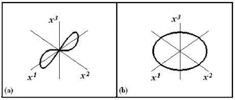
Figure 1: The figure a) on the left shows the trajectory of a charged particle in the field of a linearly polarized electromagnetic wave, whereas the figure b) on the right shows the trajectory in the field of a circularly polarized wave.

A circularly polarized wave provides an exceptional case wherein the magnetic component of the force is inactive; the particle does not have an $x^{3}$-component of motion. The trajectory of the particle, which is on average at rest, is given by [9],

$$\begin{array}[]{c}x^{1}=-\frac{eE}{m\omega^{2}}\cos{\omega t},\ \ \ x^{2}=-\frac{eE}{m\omega^{2}}\sin{\omega t},\ \ \ x^{3}=0.\end{array}$$ (6)

The particle moves in the $(x^{1},x^{2})$ plane along a circle, as shown in Fig. 1b. In the general case of an elliptically-polarized wave, the $x^{3}$-component of motion is always present. The projection of the trajectory onto the $(x^{1},x^{2})$ plane forms an ellipse. The ellipse degenerates into a straight line or a circle for a linearly-polarized or a circularly-polarized wave, respectively. We shall see below that there exists an analogy between the considered motion of charged particles in the field of an electromagnetic wave and the motion of test masses in the field of a gravitational wave.

3 Motion of a free test mass in the field of a weak gravitational wave

Weak gravitational waves belong to the class of weak gravitational fields:

$$ds^{2}=c^{2}dt^{2}-\left[\delta_{ij}+h_{ij}\right]dx^{i}dx^{j}.$$ (7)

A general expression for a plane wave incoming from the positive $x^{3}$ direction is given by

$$h_{ij}={\stackrel{{\scriptstyle 1}}{{p}}_{ij}}a+{\stackrel{{\scriptstyle 2}}{{p}}_{ij}}b,$$ (8)

where

$$\begin{array}[]{l}a=h_{+}\sin{\left(k({x^{0}}+{x^{3}})+\psi_{+}\right)},\ \ \ b=h_{\times}\sin{\left(k({x^{0}}+{x^{3}})+\psi_{\times}\right)},\end{array}$$ (10)

and $k=\frac{2\pi}{\lambda}=\frac{2\pi\nu}{c}=\frac{\omega}{c}$, $x^{0}=ct$; $\psi_{+}$ and $\psi_{\times}$ are arbitrary phases. The polarization tensors ${\stackrel{{\scriptstyle s}}{{p}}_{ij}}$ $(s=1,2)$ are given by

$$\begin{array}[]{l}{\stackrel{{\scriptstyle 1}}{{p}}_{ij}}=m_{i}m_{j}-n_{j}n_{i},\ \ \ \ {\stackrel{{\scriptstyle 2}}{{p}}_{ij}}=-m_{i}n_{j}-m_{j}n_{i},\end{array}$$ (12)

where the unit vectors $m_{i}$ and $n_{i}$, together with the unit vector $k_{3}/k$ pointing out in the direction of the wave propagation, form a triplet of mutually orthogonal unit vectors.

One still has the freedom of turning the coordinate system in the ($x^{1},x^{2}$) plane by some angle. This transformation mixes the components of the matrix (8). Using this freedom (see A) one can simplify the functions (10) in such a way that in the new coordinate system they take the form

$$\begin{array}[]{l}a=h_{+}\sin{\left(k({x^{0}}+{x^{3}})+\psi\right)},\ \ \ b=h_{\times}\cos{\left(k({x^{0}}+{x^{3}})+\psi\right)},\end{array}$$ (14)

where $h_{+},~{}h_{\times}$ are arbitrary amplitudes and $\psi$ is an arbitrary phase. The unit vectors $m_{i},~{}n_{i}$ have the components $m_{i}=1,0,0$ and $n_{i}=0,1,0$. We shall call this special coordinate system a frame based on principal axes. Two independent linear polarization states are defined by the conditions $h_{+}=0$ or $h_{\times}=0$, and two independent states of circular polarization are defined by $h_{+}=h_{\times}$ or $h_{+}=-h_{\times}$. Specifically, we will be working with the metric

$$ds^{2}=c^{2}dt^{2}-(1+a)d{x^{1}}^{2}-(1-a)d{x^{2}}^{2}+2b~{}d{x^{1}}d{x^{2}}-d{x^{3}}^{2},$$ (15)

where the functions $a$ and $b$ are given by Eq. (14).

The metric (15) is written in synchronous coordinates. Therefore, the world lines ${x^{1}},{x^{2}},{x^{3}}=const$ are time-like geodesics, they represent the histories of free test masses. To be as close as possible to the framework of laboratory physics, and specifically to electrodynamic examples considered in the previous section, we have to introduce a local inertial coordinate system $(\bar{t},{\bar{x}^{1}},{\bar{x}^{2}},{\bar{x}^{3}})$. Let us associate it with the central world line ${x^{1}}={x^{2}}={x^{3}}=0$. By definition, in the local inertial frame, and along the central geodesic line, the metric tensor takes on the Minkowski values and all first derivatives of the metric tensor vanish. The transformed metric takes on the form

$$\bar{g}_{\mu\nu}=\eta_{\mu\nu}+{\it terms~{}of~{}the~{}order~{}of}~{}\left(h\frac{{\overline{x}^{1}}^{2}+{\overline{x}^{2}}^{2}+{\overline{x}^{3}}^{2}}{\lambda^{2}}\right).$$ (16)

A local inertial frame realizes, as good as we can do in the presence of the gravitational field, a rigid freely falling “box” with a clock in it [10]. The required coordinate transformation ${\bar{x}}^{\mu}={\bar{x}}^{\mu}\left(x^{\nu}\right)$ is given by [8]:

$$\begin{array}[]{l}{\bar{x}^{0}}=x^{0}+\frac{1}{4}\dot{a}~{}\left({x^{1}}^{2}-{x^{2}}^{2}\right)-\frac{1}{2}\dot{b}~{}{x^{1}}{x^{2}},\\ \\ {\bar{x}^{1}}={x^{1}}+\frac{1}{2}a~{}{x^{1}}-\frac{1}{2}b~{}{x^{2}}+\frac{1}{2}\dot{a}~{}{x^{3}}{x^{1}}-\frac{1}{2}\dot{b}~{}{x^{3}}{x^{2}},\\ \\ {\bar{x}^{2}}={x^{2}}-\frac{1}{2}a~{}{x^{2}}-\frac{1}{2}b~{}{x^{1}}-\frac{1}{2}\dot{a}~{}{x^{3}}{x^{2}}-\frac{1}{2}\dot{b}~{}{x^{3}}{x^{1}},\\ \\ {\bar{x}^{3}}={x^{3}}-\frac{1}{4}\dot{a}~{}\left({x^{1}}^{2}-{x^{2}}^{2}\right)+\frac{1}{2}\dot{b}~{}{x^{1}}{x^{2}}.\end{array}$$ (24)

In the above transformation, the functions $a$, $b$ and their time derivatives $\dot{a}=\frac{1}{c}\frac{\partial a}{\partial t}$, $\dot{b}=\frac{1}{c}\frac{\partial b}{\partial t}$ are evaluated along the world line ${x^{1}}={x^{2}}={x^{3}}=0$. The linear and quadratic terms, as powers of $x^{\alpha}$, are unambiguously determined by the conditions of local inertial frame, but the cubic and higher-order corrections are not determined by these conditions. In principle, transformations (24) can be used for all values of $x^{\alpha}$, but they are physically useful when the values of $x^{\alpha}$ are sufficiently small, that is, when the cubic and higher-order terms can be neglected.

Let us consider a free test mass riding on a time-like geodesic (${x^{1}=l_{1}}$, ${x^{2}=l_{2}}$, ${x^{3}=l_{3}}$). Equations (24) define the behaviour of this mass with respect to the introduced local inertial frame. Concretely, we have

$$\begin{array}[]{l}{\bar{x}^{1}}(t)={l_{1}}+\frac{1}{2}\left[h_{+}{l_{1}}\sin{(\omega t+\psi)}-h_{\times}{l_{2}}\cos{(\omega t+\psi)}\right]\\ \\ ~{}\ \qquad+\frac{1}{2}k\left[h_{+}{l_{3}}{l_{1}}\cos{(\omega t+\psi)}+h_{\times}{l_{3}}{l_{2}}\sin{(\omega t+\psi)}\right],\\ \\ {\bar{x}^{2}}(t)={l_{2}}-\frac{1}{2}\left[h_{+}{l_{2}}\sin{(\omega t+\psi)}+h_{\times}{l_{1}}\cos{(\omega t+\psi)}\right]\\ \\ ~{}\ \qquad-\frac{1}{2}k\left[h_{+}{l_{3}}{l_{2}}\cos{(\omega t+\psi)}-h_{\times}{l_{3}}{l_{1}}\sin{(\omega t+\psi)}\right],\\ \\ {\bar{x}^{3}}(t)={l_{3}}-\frac{1}{4}k\left[h_{+}\left({l_{1}}^{2}-{l_{2}}^{2}\right)\cos{(\omega t+\psi)}+2h_{\times}{l_{1}}{l_{2}}\sin{(\omega t+\psi)}\right].\end{array}$$ (34)

Obviously, the unperturbed (i.e. in the absence of the gravitational wave) position of the nearby mass is $({l_{1}},{l_{2}},{l_{3}})$. The action of the wave drives the mass in an oscillatory fashion around the unperturbed position. In general, all three components of motion are present.

If one neglects in Eq. (34) the terms with $k$, thus effectively sending the wavelength $\lambda$ to infinity, one arrives at the often cited statement about the particle’s motion:

$$\begin{array}[]{l}{\bar{x}^{1}}(t)={l_{1}}+\frac{1}{2}\left[h_{+}{l_{1}}\sin{(\omega t+\psi)}-h_{\times}{l_{2}}\cos{(\omega t+\psi)}\right],\\ \\ {\bar{x}^{2}}(t)={l_{2}}-\frac{1}{2}\left[h_{+}{l_{2}}\sin{(\omega t+\psi)}+h_{\times}{l_{1}}\cos{(\omega t+\psi)}\right],\\ \\ {\bar{x}^{3}}(t)={l_{3}}.\end{array}$$ (40)

Clearly, this is the analog of the electric component of motion in electrodynamics; moving particles remain in the plane of the wave-front. The oscillations of individual particles, for the particular case of a linearly polarized g.w., are shown in Fig. 2.

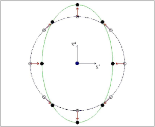
Figure 2: Motion of free test masses in the field of a linearly polarized ($h_{+}\neq 0,h_{\times}=0$) g.w. in the lowest approximation, that is, when the wave number $k$ is effectively set to zero.

A circular disk, consisting of particles that are located in the plane of the wave-front, stretches and squeezes in an oscillatory fashion, as shown in Fig.3.

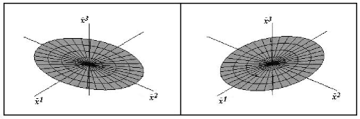
Figure 3: Deformation of a disk of free test particles in the field of a linearly polarized ($h_{+}\neq 0,h_{\times}=0$) g.w. in the limit of $k=0$. The two figures show the displacements at the moments of time separated by a half period.

Now, let us take into account the terms with $k$ in Eq. (34). If $l_{3}=0$, these terms do not change the ${\bar{x}^{1}},{\bar{x}^{2}}$ components of motion, but nevertheless they introduce oscillations along the ${\bar{x}^{3}}$ direction. In analogy with electrodynamics, it is reasonable to call these terms the “magnetic” components of motion. The trajectories of free masses are, in general, ellipses, and they are not confined to the plane of the wave-front. In Fig. 4 (taken from [8]) we show the trajectories of some individual particles. The “magnetic” contribution is smaller than the “electric” one. In analogy with electrodynamics, the major axis of the individual ellipse is small in comparison with $\lambda$ and $l$, but the size of the ${\bar{x}^{3}}$-amplitude is even smaller than the ${\bar{x}^{1}}$-amplitude. Their ratio is typically of the order of $kl=2\pi(l/\lambda)$, where $l=\sqrt{{l_{1}}^{2}+{l_{2}}^{2}+{l_{3}}^{2}}$ is the mean (unperturbed) distance of the test particle from the origin. In analogy with electrodynamics, the “magnetic” component of motion will be present even if the particle is initially at rest with respect to the local inertial frame.

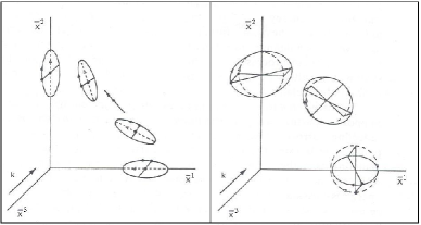
Figure 4: Solid lines show 3-dimensional motion of particles, while dashed lines show projections of the trajectories onto the $\bar{x}^{1},\bar{x}^{2}$ plane. In the left picture the wave is linearly polarized ($h_{+}\neq 0,h_{\times}=0$), whereas in the right picture the wave is circularly polarized ($h_{+}=h_{\times}$).

A circular disk, consisting of free test particles, also behaves differently, as compared with the lowest order “electric” approximation. The disk does not remain flat while being stretched and squeezed. In addition to being stretched and squeezed it bends, in an oscillatory manner, forward and backward in the ${\bar{x}^{3}}$ direction. We show these complicated deformations in Fig. 5. The level of the “magnetic” contribution is determined by the assumption that $l/\lambda=0.1$. This figure should be compared with Fig. 3.

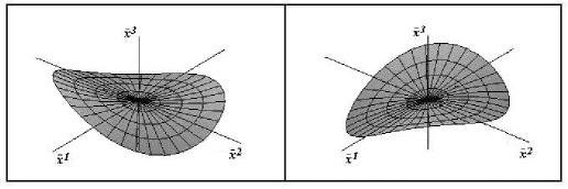
Figure 5: The figure shows the deformations of a circular disk of free test particles under the action of a linearly polarized g.w. ($h_{+}\neq 0,h_{\times}=0$). The “magnetic” contribution is responsible for the displacements along the ${\bar{x}^{3}}$ axis. The two pictures show the configurations at the moments of time separated by a half of period.

4 Equations of motion from the geodesic deviation equations.

In this section we shall consider the motion of free masses from a different perspective. The geodesic deviation equations will be used in order to derive the analog of the Lorentz force Eq. (1) and the analog of the Newtonian equations of motion Eq. (2). We shall see that the “magnetic” component of motion is contained in the higher-order geodesic deviation equations.

4.1 Geodesic deviation equations in general

The derivation of the geodesic deviation equations is usually based on a 2-parameter family of time-like geodesics $x^{\mu}(\tau,r)$. For each value of $r$, the line $x^{\mu}(\tau,r)$ is a time-like geodesic with a proper time parameter $\tau$. The vector $u^{\mu}$ is the unit tangent vector to the geodesic, and $n^{\mu}$ is the “separation” vector between the geodesics (see Fig. 6):

$$u^{\mu}(\tau,r)=\frac{\partial x^{\mu}}{\partial\tau}|_{r=const}~{},~{}~{}~{}n^{\mu}(\tau,r)=\frac{\partial x^{\mu}}{\partial r}|_{\tau=const}~{}.$$ (41)

Let the central (fiducial) geodesic line correspond to $r=0$, and a nearby geodesic to $r=r_{0}$. For small $r_{0}$, one has:

$$x^{\mu}(\tau,r_{0})=x^{\mu}(\tau,0)+r_{0}\frac{\partial x^{\mu}}{\partial r}+\frac{1}{2}r_{0}^{2}\frac{\partial^{2}x^{\mu}}{{\partial r}^{2}}+O(r_{0}^{3}).$$ (42)

Then, in the lowest approximation in terms of $r_{0}$, the geodesic deviation equations are given by [10]:

$$\frac{D^{2}n^{\mu}}{d\tau^{2}}=R^{\mu}_{\alpha\beta\gamma}u^{\alpha}u^{\beta}n^{\gamma},$$ (43)

where $R^{\mu}_{\alpha\beta\gamma}$ is the curvature tensor calculated along the geodesic line $r=0$, and $\frac{D}{d\tau}$ is the covariant derivative calculated along that line.

To discuss the “magnetic” component of motion in the field of a gravitational wave we will need the geodesic deviation equations extended to the next approximation. These equations were derived by Bazanski [11]. A modified derivation can be found in [12]. In the required approximation, one needs the information on the second derivatives of $x^{\mu}$: $\frac{\partial^{2}x^{\mu}}{{\partial r}^{2}}$. These quantities do not form a vector. It is convenient to introduce a closely related vector $w^{\mu}$:

$$w^{\mu}=\frac{Dn^{\mu}}{dr}=n^{\mu}_{;\alpha}n^{\alpha}=\frac{\partial^{2}x^{\mu}}{{\partial r}^{2}}+\Gamma^{\mu}_{\alpha\beta}n^{\alpha}n^{\beta}.$$ (44)

This vector obeys the equations [11] (see also [12]):

$$\frac{D^{2}w^{\mu}}{d\tau^{2}}=R^{\mu}_{\alpha\beta\gamma}u^{\alpha}u^{\beta}w^{\gamma}+\left(R^{\mu}_{\alpha\beta\gamma;\delta}-R^{\mu}_{\gamma\delta\alpha;\beta}\right)u^{\alpha}u^{\beta}n^{\gamma}n^{\delta}+4R^{\mu}_{\alpha\beta\gamma}u^{\beta}\frac{Dn^{\alpha}}{d\tau}n^{\gamma}.$$ (45)

To combine equations (43) and (45) into a single formula, valid up to and including the terms of the order of $r_{0}^{2}$, it is convenient to construct a vector $N^{\mu}$:

$$N^{\mu}=r_{0}n^{\mu}+\frac{1}{2}r_{0}^{2}w^{\mu}.$$ (46)

Taking the sum of Eq. (43), multiplied by $r_{0}$, and Eq. (45) multiplied by $r_{0}^{2}/2$, we obtain the equation whose solution we will need,

$$\frac{D^{2}N^{\mu}}{d\tau^{2}}= R^{\mu}_{\alpha\beta\gamma}u^{\alpha}u^{\beta}N^{\gamma}+\frac{1}{2}\left(R^{\mu}_{\alpha\beta\gamma;\delta}-R^{\mu}_{\gamma\delta\alpha;\beta}\right)u^{\alpha}u^{\beta}N^{\gamma}N^{\delta}$$ (47)

$$+2R^{\mu}_{\alpha\beta\gamma}u^{\beta}\frac{DN^{\alpha}}{d\tau}N^{\gamma}+O(r_{0}^{3}).$$

In terms of $N^{\mu}$, the expansion (42) takes the form

$$x^{\mu}(\tau,r_{0})=x^{\mu}(\tau,0)+N^{\mu}-\Gamma^{\mu}_{\alpha\beta}N^{\alpha}N^{\beta}+O(r_{0}^{3}).$$ (48)

Formula (48) shows that in the local inertial frame (in which case ${\Gamma}^{\mu}_{\alpha\beta}=0$ along the central geodesic line) the spatial components $N^{i}$ will directly give the time-dependent positions of the nearby particle. According to Eq. (47), these positions include the next order corrections, as compared with solutions to Eq. (43).

In Fig 6 we show the successive approximations to the exact position of the nearby geodesic $(b)$. The line $(d)$ represents the first order approximation (i.e. $x^{\mu}(\tau,r_{0})=x^{\mu}(\tau,0)+r_{0}\frac{\partial x^{\mu}}{\partial r}$ ), the line $(c)$ takes into account the second order approximation (i.e. $x^{\mu}(\tau,r_{0})=x^{\mu}(\tau,0)+r_{0}\frac{\partial x^{\mu}}{\partial r}+\frac{1}{2}r_{0}^{2}\frac{\partial^{2}x^{\mu}}{{\partial r}^{2}}$ ), according to (42).

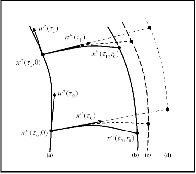
Figure 6: Deviation of two nearby geodesics in a gravitational field. Line (a) represents the central geodesic $r=0$ and line (b) represents the nearby geodesic $r=r_{0}$. $u^{\mu}$ is the unit tangent vector to the central world line, $n^{\mu}$ is the tangent vector to the curve $\tau=const$. The lines (d) and (c) are the corresponding first and second order approximations to the exact nearby geodesic (b).

4.2 Geodesic deviation in the field of a gravitational wave

We now specialize to the g.w. metric (7), (8), where $a$ and $b$ are given by (14). We take account only of linear perturbations in terms of g.w. amplitude $h$. The first particle is described by the central time-like geodesic $x^{i}(t)=0$, its tangent vector is $u^{\alpha}=(1,0,0,0)$. The second particle resides at the unperturbed position $x^{i}(0)=l^{i}$ and has zero unperturbed velocity. It is assumed that the local inertial frame is realized along the central geodesic. The objective is to find the trajectory of the second particle using the geodesic deviation equation (47).

The deviation vector $N^{i}$ has the form

$${N}^{i}(t)=l^{i}+\xi^{i}(t),$$ (49)

where $\xi^{i}(t)$ is the perturbation caused by the gravitational wave. The choice of the local inertial frame allows one to replace all covariant derivatives in Eq. (47) by ordinary derivatives. In particular, covariant time derivative $\frac{D^{2}}{d\tau^{2}}$ is being replaced by ordinary time derivative $\frac{d^{2}}{c^{2}dt^{2}}$. In the lowest approximation, Eqs. (47) reduce to Eqs. (43) and specialize to

$$\frac{d^{2}\xi^{i}}{dt^{2}}=-\frac{1}{2}l^{j}\frac{\partial^{2}}{{\partial t}^{2}}\left({h^{i}_{j}}\right)=\frac{1}{2}\omega^{2}l^{j}\left[{\stackrel{{\scriptstyle 1}}{{p}}{}_{j}^{i}}h_{+}\sin(\omega t+\psi)+{\stackrel{{\scriptstyle 2}}{{p}}{}_{j}^{i}}h_{\times}\cos(\omega t+\psi)\right].$$ (50)

As expected, the relevant solution to this equation coincides exactly with the usual “electric” part of the motion, which is given by Eq. (40).

In order to identify the “magnetic” part of the gravitational force, one has to consider all the terms in Eq. (47). Since $DN^{\alpha}/d\tau$ is of the order of $h$, the third term in Eq. (47) is of the order of $h^{2}$ and should be neglected. Working out the derivatives of the curvature tensor and substituting them into (47), we arrive at the accurate equations of motion:

$$\frac{d^{2}\xi^{i}}{dt^{2}}=-\frac{1}{2}l^{j}\frac{\partial^{2}}{{\partial t}^{2}}\left(h^{i}_{j}\right)-\frac{1}{2}l^{k}l^{l}\frac{\partial^{2}}{{\partial t}^{2}}\left(\frac{\partial}{\partial x^{l}}\left(h^{i}_{k}\right)-\frac{1}{2}\delta^{ij}\frac{\partial}{\partial x^{j}}\left(h_{kl}\right)\right).$$ (51)

The second term of this formula is responsible for the “magnetic” component of motion and can be interpreted as the gravitational analog of the magnetic part of the Lorentz force (1).

Specifically, in the field of the gravitational wave (15), the full equations of motion (51) take the form:

$$\frac{d^{2}\xi^{i}}{dt^{2}}= \frac{1}{2}\omega^{2}l^{j}\left[{\stackrel{{\scriptstyle 1}}{{p}}{}_{j}^{i}}h_{+}\sin(\omega t+\psi)+{\stackrel{{\scriptstyle 2}}{{p}}{}_{j}^{i}}h_{\times}\cos(\omega t+\psi)\right]$$ (52)

$$-\frac{1}{2}\omega^{2}l^{k}l^{l}\left[k_{l}\delta^{ij}+\frac{1}{2}k^{i}\delta^{j}_{l}\right]\left[{\stackrel{{\scriptstyle 1}}{{p}}{}_{kj}}h_{+}\cos(\omega t+\psi)-{\stackrel{{\scriptstyle 2}}{{p}}{}_{kj}}h_{\times}\sin(\omega t+\psi)\right].$$

This equation clearly exhibits two contributions:

$$m\frac{d^{2}\xi^{i}}{dt^{2}}=F_{(e)}^{i}+F_{(m)}^{i}.$$ (53)

The “electric” component of the gravitational force $F_{(e)}^{i}/m$ is given by the first term in Eq. (52). The second term - the “magnetic” component $F_{(m)}^{i}/m$ of the gravitational force - can be written, demonstrating certain analogy with electrodynamics, in the form involving the (lowest order non-vanishing) velocity $\frac{d\xi^{i}}{dt}$ of the test particle:

$$\frac{F_{(m)}^{i}}{m}=\omega l^{l}\left[k_{l}\delta^{i}_{j}+\frac{1}{2}k^{i}\delta_{jl}\right]\frac{d\xi^{j}}{dt}.$$ (54)

The right hand side of Eq. (52) is exactly the acceleration $\frac{d^{2}\bar{x}^{i}}{dt^{2}}$ which can be derived by taking the time derivatives of Eq. (34). Not surprisingly, by integrating equations of motion (52), one arrives exactly at the time-dependent positions of the particles, Eq. (34), which we have already derived by the direct coordinate transformation. Therefore, the gravitational Lorentz force, identified above, leads exactly to the expected result.

It should be noted that Eqs. (52) depend only on the so-called TT-components of the g.w. field. This happens not only because we have explicitly started from them in Eq. (15). Even if we have started from the general form of the g.w. field, which includes also the non-TT components, we would have ended up with equations containing only the TT-components. This happens because Eqs. (47) involve the curvature tensor (and its derivatives) in which the non-TT components automatically cancel out.

It is interesting to compare the components of the gravitational force derived here with what would follow from the concept of “gravitomagnetism”. In general, the concept of “gravitomagnetism” is a helpful analogy which was successfully used in studies of stationary gravitational fields [13], [14]. However, its application to the gravitational-wave problem considered here requires certain care. For example, in the local inertial frame, the leading terms of the equations of motion derived in the framework of “gravitomagnetism” [14] read (in notations consistent with this paper):

$$\frac{d^{2}N^{i}}{dt^{2}}=R^{i}_{00j}N^{j}+2R^{i}_{j0k}\frac{dN^{j}}{dt}N^{k}.$$ (55)

This equation should be compared with our Eq. (47), also specialized to the local inertial frame:

$$\frac{d^{2}N^{i}}{dt^{2}}=R^{i}_{00j}N^{j}+\frac{1}{2}\left(R^{i}_{00j;k}-R^{i}_{jk0;0}\right)N^{j}N^{k}+2R^{i}_{j0k}\frac{dN^{j}}{dt}N^{k}.$$ (56)

Clearly, the last term in both equations is common, and it resembles the magnetic part of the electromagnetic Lorentz force. However, as was shown above, for particles which do not have large unperturbed velocities and are (on average) at rest in the local inertial frame, this term is quadratic in $h$ and should be neglected. At the same time, the second term in Eq. (56) (which we provisionally call “magnetic”) is linear in $h$ and cannot be neglected. Regardless of terminology, the correct results exhibited in Eq. (34) can only be obtained if one proceeds with Eq. (56) and not with Eq. (55).

5 Variation of the distance between test masses

We have used a local inertial frame and completely specified the time-dependent positions of test particles acted upon by a gravitational wave. As was already mentioned, this description is as close as possible to the description of laboratory physics. Having answered all the questions with regard to particles’s positions, we can now discuss the variation of distances between them. We are mostly interested in the distance between the central particle and the particle located, on average, at some position $(l_{1},l_{2},l_{3})$. This is a model for the central mirror and the end-mirror placed in one of the arms of an interferometer. We will later use these results for the derivation of the response function of the laser interferometer.

In the local inertial frame, metric tensor (16) has the Minkowski values up to small terms of order of $h(\frac{l}{\lambda})^{2}$. The Euclidian expression

$$d(t)=\sqrt{{\overline{x}^{1}}^{2}+{\overline{x}^{2}}^{2}+{\overline{x}^{3}}^{2}}+O\left(hl(l/\lambda)^{2}\right),$$ (57)

gives the distance between particles, which is accurate up to terms of the order of $hl$ and $hl\frac{l}{\lambda}$ inclusive. Obviously, we neglect the terms quadratic in $h$. Denoting ${\bar{x}^{i}}=l_{i}+\Delta{\bar{x}^{i}}$, one gets

$$d(t)\approx l+\frac{1}{l}\left(l_{1}\Delta{\bar{x}^{1}}+l_{2}\Delta{\bar{x}^{2}}+l_{3}\Delta{\bar{x}^{3}}\right).$$ (58)

Using the time-dependent positions (34), we obtain the distance $d(t)$ with the required accuracy:

$$d(t)= l+\frac{1}{2l}\left[h_{+}({l_{1}}^{2}-{l_{2}}^{2})\sin{(\omega t+\psi)}-2h_{\times}{l_{1}}{l_{2}}\cos{(\omega t+\psi)}\right]$$

$$+\frac{1}{4l}kl_{3}\left[h_{+}({l_{1}}^{2}-{l_{2}}^{2})\cos{(\omega t+\psi)}+2h_{\times}{l_{1}}{l_{2}}\sin{(\omega t+\psi)}\right]+O\left(hl(l/\lambda)^{2}\right).$$

Clearly, the first correction to $l$ is due to the “electric” contribution, whereas the second correction to $l$ is due to the “magnetic” contribution.

According to Eqs. (34), the “magnetic” component of motion is present even if the mean position of the second mass is such that $l_{3}=0$. However, this motion is in the direction orthogonal to the line joining the masses and therefore it does not lead to a (first order in terms of $h$) change of distance between them. This fact is reflected in Eq. (LABEL:deltar12) in the form of disappearance of the “magnetic” contribution to the distance when $l_{3}=0$. In other words, “magnetic” contribution to the distance is present only if the interferometer’s arm is not orthogonal to the wave’s propagation.

The distance (LABEL:deltar12) was calculated in the local inertial frame. It was assumed that $l/\lambda\ll 1$. It is important to show that the approximate expression (LABEL:deltar12) follows also from exact definitions of distance. One of them is based on the measurement of time that it takes for a light ray to travel from one free particle to another and back. [This is a part of a more general problem of finding light-like geodesics in the presence of a weak gravitational wave [10],[15], [16].] This definition is applicable regardless of the relationship between $l$ and $\lambda$ and does not require the introduction of a local inertial frame. If a photon is sent out from the first particle-mirror at the moment of time $t_{0}$, gets reflected off the second particle-mirror, and then returns back to the first particle-mirror at $t_{2}$, the proper distance $d(t)$ between the mirrors at time $t$ is defined as

$$d\left(t\right)=c\frac{t_{2}-t_{0}}{2},$$ (60)

where $t=(t_{0}+t_{2})/2$ is the mean time between the departure of the photon and its arrival back.

In the field of the gravitational wave (15), the light rays, $ds^{2}=0$, are described by the equation

$$c^{2}dt^{2}=(1+a)d{x^{1}}^{2}+(1-a)d{x^{2}}^{2}-2b~{}d{x^{1}}d{x^{2}}+d{x^{3}}^{2}.$$ (61)

Let the (unperturbed) outgoing light ray be parameterized as

$$x^{0}=ct_{0}+l\tau,~{}~{}~{}x^{1}=l_{1}\tau,~{}~{}~{}x^{2}=l_{2}\tau,~{}~{}~{}x^{3}=l_{3}\tau,$$ (62)

where the parameter $\tau$ changes from 0 to 1. Then, according to Eq. (61), we have along the ray:

$$cdt=l\left[1+\frac{1}{2}a(\tau)\frac{l_{1}^{2}-l_{2}^{2}}{l^{2}}-b(\tau)\frac{l_{1}l_{2}}{l^{2}}\right]d\tau.$$ (63)

Integrating both parts of this equation, we can find the time $t$ of arrival of the photon to the second particle. The calculated time includes the g.w. corrections proportional to $h_{+}$ and $h_{\times}$. Similarly, the (unperturbed) reflected light ray can be parameterized as

$$x^{0}=ct+l\tau,~{}~{}~{}x^{1}=l_{1}-l_{1}\tau,~{}~{}~{}x^{2}=l_{2}-l_{2}\tau,~{}~{}~{}x^{3}=l_{3}-l_{3}\tau,$$ (64)

where $\tau$ is again changing from 0 to 1. A similar integration of Eq. (63) allows us to find the time $t_{2}$ of arrival of the photon back to the first particle, including the g.w. corrections.

Combining two pieces of the light travel time, we derive the exact formula for the distance:

$$d(t)=l+\frac{1}{2l}\left[h_{+}\frac{l_{1}^{2}-l_{2}^{2}}{2}{\Phi}_{c}+h_{\times}l_{1}l_{2}\Phi_{s}\right],$$ (65)

where

$$\Phi_{c}= -\frac{1}{k(l+l_{3})}\left[\cos{(\omega t+\psi+kl_{3})}-\cos{(\omega t+\psi-kl)}\right]$$ (66)

$$+\frac{1}{k(l-l_{3})}\left[\cos{(\omega t+\psi+kl_{3})}-\cos{(\omega t+\psi+kl)}\right],$$

and $\Phi_{s}$ is obtained from $\Phi_{c}$ by the replacement of all $\cos$-functions with $\sin$-functions of the same arguments. Exactly the same formula (65) follows also from the direct joining of the perturbed light-like geodesic lines, derived in reference [15].

Formula (LABEL:deltar12) is sufficient for ground-based interferometers, for which the condition $l\ll\lambda$ is usually satisfied. Formula (65) is appropriate for space-based interferometers for which the above condition is not satisfied in the higher-frequency portion of the sensitivity band (see, for example, [3], [17], [18], [19]). However, it is important that formula (LABEL:deltar12), including its “magnetic” terms, follows also from exact definition (65), when the appropriate approximation is taken. Assuming that $k(l+l_{3})\ll 1$ and $k(l-l_{3})\ll 1$ and retaining only the first two terms in the expansion of $\Phi_{c}$ and $\Phi_{s}$, one derives Eq. (LABEL:deltar12) from Eq. (65). As expected, the “magnetic” contribution to the distance is a universal phenomenon. It is most easily identified and interpreted in the local inertial frame, but conclusions about the distance do not depend on the introduction of this frame.

It is known that there is no unique definition of spatial distance in curved space-time. We have considered the definition based on measuring the round-trip time of a light ray. One more definition is based on measuring the length of a spatial geodesic line joining the particles at a fixed moment of time. It can be shown that this definition leads to the formula

$$d(t)=l+\frac{1}{2l}\left[h_{+}\frac{l_{1}^{2}-l_{2}^{2}}{2}{\tilde{\Phi}}_{c}+h_{\times}l_{1}l_{2}\tilde{\Phi}_{s}\right],$$ (67)

where

$$\tilde{\Phi}_{c}= -\frac{2}{kl_{3}}\left[\cos{(\omega t+\psi+kl_{3})}-\cos{(\omega t+\psi)}\right],$$ (68)

and $\tilde{\Phi}_{s}$ is obtained from $\tilde{\Phi}_{c}$ by the replacement of all $\cos$-functions with $\sin$-functions of the same arguments. In general, the distance (67) differs from the distance (65). However, they do coincide in the first order approximation in terms of small parameter $kl$. This can be shown by expanding Eq. (67) in powers of $kl$ and retaining the linear terms. It is satisfying that the exact definitions (65) and (67) lead precisely to the Euclidean result (LABEL:deltar12) in the appropriate approximation.

6 Response of an interferometer to the incoming plane gravitational wave

Laser interferometer measures the difference of distances travelled by light in two arms. We describe interferometer in the local inertial frame, with the origin of the frame at the corner mirror. The unperturbed coordinates of the end-mirrors are given by $(l^{(\textsl{a})}_{1},~{}l^{(\textsl{a})}_{2},~{}l^{(\textsl{a})}_{3})$, where $\textsl{a}=1,2$ labels the arms. We consider an interferometer whose unperturbed arms have equal lengths, $l=\sqrt{{l^{(\textsl{a})}_{1}}^{2}+{l^{(\textsl{a})}_{2}}^{2}+{l^{(\textsl{a})}_{3}}^{2}}$, and the arms are orthogonal to each other. A detailed introduction to interferometers in gravitational-wave research can be found in [2], [20], [3].

It was shown in the previous section that the distance variation in one of the arms is given by Eq. (LABEL:deltar12). Then, the response of a 2-arm interferometer is given by

$$\Delta d(t)=d(t)^{(1)}-d(t)^{(2)}.$$ (69)

The derivation of formula (LABEL:deltar12) is based on the coordinate system adjusted to the gravitational wave. Specifically, it is assumed that the $x^{3}$ axis is the direction from which the incoming plane wave propagates, while the $x^{1},x^{2}$ directions are defining the principal axes of the wave, see Eq. (15). Then, the response function (69) is characterized by six free parameters $(l^{(\textsl{a})}_{1},~{}l^{(\textsl{a})}_{2},~{}l^{(\textsl{a})}_{3})$. Among these six parameters only four are independent (one of which is $l$), because the arms have equal unperturbed lengths $l$ and are orthogonal to each other.

When it comes to the observer, it is more convenient to associate coordinate system with the interferometer’s arms, rather than with one particular wave. Let the observer’s coordinate system $({X^{1}},{X^{2}},{X^{3}})$ be chosen in such a way that the arms are located along the $X^{1}$ and $X^{2}$ directions. Then, the response function is characterized by $l$ and three angles : $\Theta$, $\Phi$ and $\Psi$. The angles $\Theta,\Phi$ describe the direction of a particular incoming wave, and the third angle $\Psi$ describes the orientation of the principal axes of the wave with respect to the observer’s meridian (see, for example, [2], [20], [21]). The relationship between these two coordinate systems is shown in Fig. 7 and is described in detail in B.

The parameters $(l^{(\textsl{a})}_{1},~{}l^{(\textsl{a})}_{2},~{}l^{(\textsl{a})}_{3})$ are expressible in terms of the parameters $\Theta,\Phi,\Psi$ according to the relationships (see B):

$$\begin{array}[]{l}l^{(1)}_{1}=l(\cos{\Phi}\cos{\Theta}\cos{\Psi}-\sin{\Phi}\sin{\Psi}),\\ l^{(1)}_{2}=l(-\sin{\Phi}\cos{\Psi}-\cos{\Phi}\cos{\Theta}\sin{\Psi}),\\ l^{(1)}_{3}=l(\cos{\Phi}\sin{\Theta}),\end{array}$$ (73)

and

$$\begin{array}[]{l}l^{(2)}_{1}=l(\sin{\Phi}\cos{\Theta}\cos{\Psi}+\cos{\Phi}\sin{\Psi}),\\ l^{(2)}_{2}=l(\cos{\Phi}\cos{\Psi}-\sin{\Phi}\cos{\Theta}\sin{\Psi}),\\ l^{(2)}_{3}=l(\sin{\Phi}\sin{\Theta}).\end{array}$$ (77)

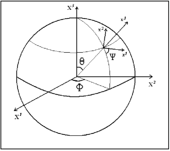
Figure 7: The relationship between the coordinate system $({x^{1}},{x^{2}},{x^{3}})$ adjusted to the wave and the coordinate system $({X^{1}},{X^{2}},{X^{3}})$ adjusted to the interferometer. The two arms of the interferometer lie along the axes $X^{1}$ and $X^{2}$.

Using (73) and (77) in (69), the response function can be written in the form

$$\Delta d(t)=l \left[~{}h_{+}\left\{F_{+}^{E}(\Theta,\Phi,\Psi)\sin(\omega t+\psi)+(kl)F_{+}^{H}(\Theta,\Phi,\Psi)\cos(\omega t+\psi)\right\}\right.$$ (78)

$$\left.+h_{\times}\left\{F_{\times}^{E}(\Theta,\Phi,\Psi)\cos(\omega t+\psi)+(kl)F_{\times}^{H}(\Theta,\Phi,\Psi)\sin(\omega t+\psi)\right\}\right],$$

where the “electric” ($E$) components of $F_{+,\times}(\Theta,\Phi,\Psi)$ are given by

$$F_{+}^{E}(\Theta,\Phi,\Psi) = \cos{2\Phi}\left(\frac{1+\cos^{2}{\Theta}}{2}\right)\cos{2\Psi}-\sin{2\Phi}\cos{\Theta}\sin{2\Psi},$$ (79)

$$F_{\times}^{E}(\Theta,\Phi,\Psi) =- \cos{2\Phi}\left(\frac{1+\cos^{2}{\Theta}}{2}\right)\sin{2\Psi}-\sin{2\Phi}\cos{\Theta}\cos{2\Psi},$$ (80)

and the “magnetic” ($H$) components of $F_{+,\times}(\Theta,\Phi,\Psi)$ are given by

$$F_{+}^{H}(\Theta,\Phi,\Psi)= \frac{1}{4}\sin{\Theta}\left[\left(\cos^{2}{\Theta}+\sin{2\Phi}\left(\frac{1+\cos^{2}{\Theta}}{2}\right)\right)\left(\cos{\Phi}-\sin{\Phi}\right)\cos{2\Psi}\right.$$ (81)

$$\left.-\frac{}{}\sin{2\Phi}\left(\cos{\Phi}+\sin{\Phi}\right)\cos{\Theta}\sin{2\Psi}\right],$$

$$F_{\times}^{H}(\Theta,\Phi,\Psi)= \frac{1}{4}\sin{\Theta}\left[\left(\cos^{2}{\Theta}+\sin{2\Phi}\left(\frac{1+\cos^{2}{\Theta}}{2}\right)\right)\left(\cos{\Phi}-\sin{\Phi}\right)\sin{2\Psi}\right.$$ (82)

$$\left.+\frac{}{}\sin{2\Phi}\left(\cos{\Phi}+\sin{\Phi}\right)\cos{\Theta}\cos{2\Psi}\right].$$

Our response function is more accurate than the previously derived expressions [2], [20], [21], [22], because our Eq. (78) includes the “magnetic” contribution. In equation (78) it is given by the terms proportional to the factor $(kl)$.

In general, the response function (78) contains two independent polarization amplitudes, $h_{+}$ and $h_{\times}$. To simplify the analysis of Eq. (78), we will separately consider circularly polarized ($h_{+}=\pm h_{\times}$), and linearly polarized ($h_{\times}=0$ or $h_{+}=0$), waves. We start with the analysis of the response function as a function of time, assuming that a circularly polarized or a linearly polarized wave arrives from a fixed direction $\Theta,\Phi$ on the sky.

In the case of a circularly polarized wave ($h_{+}=\pm h_{\times}$) we obtain

$$\Delta d(t)=l~{}h_{+}~{}{\left[{F^{E}_{+}}^{2}+{F^{E}_{\times}}^{2}\right]}^{\frac{1}{2}}\left[1\pm(kl)\left(\frac{F^{E}_{+}F^{H}_{\times}+F^{E}_{\times}F^{H}_{+}}{{F^{E}_{+}}^{2}+{F^{E}_{\times}}^{2}}\right)\right]\sin{\left(\omega t+\psi\pm\Delta\psi\right)},$$ (83)

where the phase shift $\Delta\psi$ is given by

$$\tan{\left(\Delta\psi\right)}=\frac{F^{E}_{\times}}{F^{E}_{+}}\left[1\pm(kl)\left(\frac{F^{E}_{+}F^{H}_{+}-F^{E}_{\times}F^{H}_{\times}}{F^{E}_{+}F^{E}_{\times}}\right)\right].$$ (84)

Clearly, the inclusion of “magnetic” terms changes the amplitude and the phase of $\Delta d(t)$. As an illustration, we show in Fig. 8 the response of an interferometer, as a function of time, to a circularly polarized wave $h_{+}=h_{\times}$, coming from the direction $\Theta=2\pi/3,\Phi=\pi/3$ (we have also set $\Psi=0$ to fix the phase of the response function; the amplitude of the response function does not depend on $\Psi$). The dashed curve shows the “electric” response alone, while the solid curve shows the total response, including the “magnetic” part. We have taken $l/\lambda=0.1$.

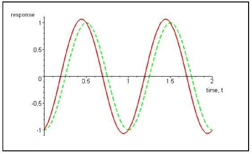
Figure 8: A typical response of an interferometer, as a function of time, to the monochromatic circularly polarized gravitational wave coming from a fixed direction on the sky. The solid line shows the total response, while the dashed line is purely “electric” part.

The response of an interferometer to any elliptically polarized wave is qualitatively similar to Fig. 8, that is, in general, the “magnetic” component contributes, both, to the amplitude and to the phase of $\Delta d(t)$. However, “magnetic” contribution to the amplitude may be very small for linearly polarized waves. If one puts $h_{\times}=0$ or $h_{+}=0$ in Eq. (78), one finds that the correction to the amplitude $\Delta d(t)$ is quadratic in $(kl)^{2}$ (and, hence, can be neglected) with the exception of directions on the sky where $F_{+}^{E}$ or $F_{\times}^{E}$ vanish. Specifically, for the linearly polarized wave $h_{\times}=0$, we obtain

$$\Delta d(t)=l~{}h_{+}~{}\sqrt{{F_{+}^{E}}^{2}+(kl)^{2}{F_{+}^{H}}^{2}}\sin{(\omega t+\psi+\Delta\psi)},$$ (85)

where the phase shift $\Delta\psi$ is given by

$$\tan{\left(\Delta\psi\right)}=kl\left(\frac{F_{+}^{H}}{F_{+}^{E}}\right).$$ (86)

(The case when $h_{+}=0$ is given by the above expressions in which all the “plus” indices are replaced by “cross” indices, and the sin-function in expression (85) is replaced by a cos-function.)

We now turn to the amplitude of $\Delta d(t)$ as a function of the angles $\Theta,\Phi$. It is usually called the beam pattern. In general, the amplitude of $\Delta d(t)$ depends also on $\Psi$, but we will consider, for simplicity, circularly polarized waves, in which case the parameter $\Psi$ does not participate in the amplitude of $\Delta d(t)$. We consider circularly polarized waves, with one and the same amplitude $h_{R}$, coming from arbitrary directions on the sky. The beam pattern is shown in Fig. 9. The left figure shows the purely “electric” contribution, whereas the right figure shows the total beam pattern, with the “magnetic” contribution included. We have taken $l/\lambda=0.1$. It is clearly seen that the “magnetic” component breaks the characteristic quadrupole symmetry of the “electric” beam pattern (more detail - in the next Section).

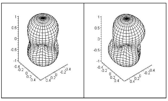
Figure 9: The amplitude of the interferometer’s response to circularly polarized waves. The graphs are normalized in such a way that the amplitude is equal 1 for $\Theta=0$. The left figure ignores the “magnetic” effect, whereas the right figure shows the total response.

7 Response function in terms of spin-weighted spherical harmonics

The response function (78) allows an elegant invariant representation in terms of the spin-weighted spherical harmonics. This description is also helpful for physical interpretation of the response function.

First, let us introduce the amplitudes of circularly polarized gravitational waves,

$$h_{R}=\frac{1}{2}\left(h_{+}+h_{\times}\right),~{}~{}~{}~{}h_{L}=\frac{1}{2}\left(h_{+}-h_{\times}\right),$$ (87)

and the complex functions

$$\begin{array}[]{l}F_{R}=\left(F_{+}^{E}+(kl)F_{\times}^{H}\right)+i\left(F_{\times}^{E}+(kl)F_{+}^{H}\right),\\ \\ F_{L}=\left(F_{+}^{E}-(kl)F_{\times}^{H}\right)+i\left(-F_{\times}^{E}+(kl)F_{+}^{H}\right).\end{array}$$ (91)

In terms of the introduced notations, the response function (78) can be identically rewritten as

$$\Delta d(t)=l\left(-\frac{i}{2}\right)\left[e^{i(\omega t+\psi)}\left(h_{R}F_{R}+h_{L}F_{L}\right)-e^{-i(\omega t+\psi)}\left(h_{R}F_{R}^{*}+h_{L}F_{L}^{*}\right)\right].$$ (92)

Clearly, the $\Delta d(t)$ has been separated in two components associated with the left (L) and right (R) polarization states of the gravitational wave. Only the $L(R)$ component of the response function is present, when the $R(L)$ g.w. amplitude is set to zero.

Using the explicit expressions (79), (80), (81) and (82), one can show that the newly defined functions $F_{R},F_{L}$ can be rearranged to read

$$F_{R}=\widetilde{F}_{R}(\Theta,\Phi)e^{-2i\Psi},~{}~{}~{}~{}F_{L}=\widetilde{F}_{L}(\Theta,\Phi)e^{2i\Psi},$$ (93)

where $\widetilde{F}_{L}$ and $\widetilde{F}_{R}$ are given by

$$\widetilde{F}_{L}= \frac{1}{4}\left[\left(1+\cos{\Theta}\right)^{2}e^{2i\Phi}+\left(1-\cos{\Theta}\right)^{2}e^{-2i\Phi}\right]$$

$$+\frac{ikl}{32}\left[(1-i)\left(1+\cos{\Theta}\right)^{2}\sin{\Theta}e^{3i\Phi}+(1+i)\left(3\cos{\Theta}-1\right)\left(\cos{\Theta}+1\right)\sin{\Theta}e^{i\Phi}\right.$$

$$\left.+(1-i)\left(3\cos{\Theta}+1\right)\left(\cos{\Theta}-1\right)\sin{\Theta}e^{-i\Phi}+(1+i)\left(1-\cos{\Theta}\right)^{2}\sin{\Theta}e^{-3i\Phi}\right],$$

$$\widetilde{F}_{R}= \frac{1}{4}\left[\left(1-\cos{\Theta}\right)^{2}e^{2i\Phi}+\left(1+\cos{\Theta}\right)^{2}e^{-2i\Phi}\right]$$

$$+\frac{ikl}{32}\left[(1-i)\left(1-\cos{\Theta}\right)^{2}\sin{\Theta}e^{3i\Phi}+(1+i)\left(3\cos{\Theta}+1\right)\left(\cos{\Theta}-1\right)\sin{\Theta}e^{i\Phi}\right.$$

$$\left.\ +(1-i)\left(3\cos{\Theta}-1\right)\left(\cos{\Theta}+1\right)\sin{\Theta}e^{-i\Phi}+(1+i)\left(1+\cos{\Theta}\right)^{2}\sin{\Theta}e^{-3i\Phi}\right].$$

For a given direction $(\Theta,\Phi)$ on the sky, the functions $F_{R}$ and $F_{L}$ transform under the rotation of $\Psi$, specified by the transformation $\Psi\rightarrow\Psi+\Psi_{0}$, according to $\widetilde{F}_{R}\rightarrow\widetilde{F}_{R}e^{-2i\Psi_{0}}$ and $\widetilde{F}_{L}\rightarrow\widetilde{F}_{L}e^{2i\Psi_{0}}$. A function ${}_{s}f(\Theta,\Phi)$ is said to be a spin-$s$ function, if under the transformation $\Psi\rightarrow\Psi+\Psi_{0}$ it transforms like ${}_{s}f(\Theta,\Phi)\rightarrow{}_{s}f(\Theta,\Phi)e^{-is\Psi_{0}}$. Therefore, our functions $F_{L}$ and $F_{R}$ represent the $s=-2$ and $s=+2$ functions, respectively.

A scalar function on a 2-sphere can be expanded over a set of ordinary spherical harmonics $Y^{l}_{m}(\Theta,\Phi)$, which form a complete and orthonormal basis. These harmonics are not appropriate for the expansion of spin-weighted functions with $s\neq 0$. The spin-weighted functions can be expanded over a set of harmonics called the spin-weighted spherical harmonics ${}_{s}{Y_{m}^{l}}(\Theta,\Phi)$ [23], [24], [25], [26]. The spin-weighted spherical harmonics satisfy the completeness and othonormality conditions similar to those of ordinary spherical harmonics. The functions ${}_{s}{Y_{m}^{l}}(\Theta,\Phi)$ can be derived from $Y^{l}_{m}(\Theta,\Phi)$ according to the rules:

$${}_{s}Y^{l}_{m}=\left\{\begin{array}[]{l}\left[\frac{(l-s)!}{(l+s)!}\right]^{1/2}\eth^{s}Y^{l}_{m},\ \ (0\leq s\leq l)\\ \\ \left(-1\right)^{s}\left[\frac{(l+s)!}{(l-s)!}\right]^{1/2}\bar{\eth}^{-s}Y^{l}_{m},\ \ (0\geq s\geq-l)\end{array}\right.,$$ (99)

where the differential operators $\eth$ and $\bar{\eth}$ [acting on a spin $s$ function ${}_{s}f(\Theta,\Phi)$] are given by

$$\begin{array}[]{l}\eth~{}{}_{s}f(\Theta,\Phi)=-\sin^{s}{\Theta}\left(\frac{\partial}{\partial\Theta}+\frac{i}{\sin{\Theta}}\frac{\partial}{\partial\Phi}\right)\sin^{-s}{\Theta}~{}{}_{s}f(\Theta,\Phi),\\ \\ \bar{\eth}~{}{}_{s}f(\Theta,\Phi)=-\sin^{-s}{\Theta}\left(\frac{\partial}{\partial\Theta}-\frac{i}{\sin{\Theta}}\frac{\partial}{\partial\Phi}\right)\sin^{s}{\Theta}~{}{}_{s}f(\Theta,\Phi).\end{array}$$ (103)

Using the spin-weighted spherical harmonics, the functions $\widetilde{F}_{L}$ and $\widetilde{F}_{R}$ can be expanded as follows:

$$\widetilde{F}_{L}= \sqrt{2\pi}\left[{}_{-2}Y^{2}_{2}(\Theta,\Phi)+{}_{-2}Y^{2}_{-2}(\Theta,\Phi)\right]$$ (104)

$$+ikl\sqrt{\frac{\pi}{46}}\left[~{}~{}\frac{(1-i)}{\sqrt{3}}{}_{-2}Y^{3}_{3}(\Theta,\Phi)+\frac{(1+i)}{\sqrt{5}}{}_{-2}Y^{3}_{1}(\Theta,\Phi)\right.$$

$$\qquad\qquad\left.+\frac{(1-i)}{\sqrt{5}}{}_{-2}Y^{3}_{-1}(\Theta,\Phi)+\frac{(1+i)}{\sqrt{3}}{}_{-2}Y^{3}_{-3}(\Theta,\Phi)\right],$$

$$\widetilde{F}_{R}= \sqrt{2\pi}\left[{}_{2}Y^{2}_{2}(\Theta,\Phi)+{}_{2}Y^{2}_{-2}(\Theta,\Phi)\right]$$ (105)

$$+ikl\sqrt{\frac{\pi}{46}}\left[~{}~{}\frac{(1-i)}{\sqrt{3}}{}_{2}Y^{3}_{3}(\Theta,\Phi)+\frac{(1+i)}{\sqrt{5}}{}_{2}Y^{3}_{1}(\Theta,\Phi)\right.$$

$$\qquad\qquad\left.+\frac{(1-i)}{\sqrt{5}}{}_{2}Y^{3}_{-1}(\Theta,\Phi)+\frac{(1+i)}{\sqrt{3}}{}_{2}Y^{3}_{-3}(\Theta,\Phi)\right].$$

As one could expect, the “electric” components of the response function are described by the spin 2 quadrupole (l=2) terms ${}_{\pm 2}Y^{2}_{m}$, whereas the “magnetic” components are described by the spin 2 octupole (l=3) terms ${}_{\pm 2}Y^{3}_{m}$. The “magnetic” components can be viewed as the higher-order terms in the multipole expansion of the response function.

8 Astrophysical example

The “magnetic” component in the motion of free masses will have serious practical implications for the current gravitational wave observations. For example, the LIGO interferometers have the arm length of $l=4km$ and are most sensitive to g.w. in the interval of frequencies between $30Hz$ and $10^{4}Hz$. This means that the “magnetic” component, whose relative contribution is of the order of $kl$, may provide a correction at the level of $5\%$ to the response function in the frequency region of $600Hz$, and up to $10\%$ in the frequency region of $1200Hz$. This contribution may significantly affect the determination of the source’s parameters.

The high frequency region, $600Hz-1200Hz$, will be extensively studied with the help of the “narrow-band tuning” of advanced interferometers [5]. The signal recycling technique allows reshaping of the sensitivity curve in such a way that it reduces noise within a chosen narrow band, while weakening sensitivity in other frequency regions. This region of high frequencies is populated by various periodic and quasi-periodic astrophysical sources, such as neutron stars in low-mass X-ray binaries, including Sco X-1, slightly deformed rotating neutron stars, neutron star and black hole binaries in the last moments of their inspiral. For a more detailed list of high frequency sources and the prospects of their detection see [5].

To better understand the role of the “magnetic” components in estimation of the g.w. source parameters, we shall briefly consider an idealized example of a compact binary system. Let the binary consist of objects of equal mass $M$ orbiting each other in a circular orbit of size $2r$. The distance of the binary to the observer is $R$. For simplicity, we assume that the orbital plane is orthogonal to the line of sight defined by $\Theta,\Phi$. Then, the gravitational wave at Earth has the form of Eq. (14) with the amplitudes given by [20], [4]:

$$\begin{array}[]{l}h_{+}=h_{\times}=h_{R}=\frac{32\pi^{2}G}{Rc^{4}}Mr^{2}\omega^{2},\end{array}$$ (107)

where the g.w. angular frequency $\omega=\sqrt{\frac{GM}{r^{3}}}$ is twice the orbital frequency. The angle $\Psi$ can be taken as $\Psi=0$, and the phase $\psi$ is the angle between the observer’s meridian and the line joining the components of the binary at some initial moment of time.

The response of the interferometer to the incoming wave is determined by Eq. (78):

$$\Delta d(t) =lh_{R}~{}\left[\left\{\cos{2\Phi}\left(\frac{1+\cos^{2}{\Theta}}{2}\right)-\frac{1}{4}\frac{\omega l}{c}\sin{2\Phi}\left(\cos{\Phi}+\sin{\Phi}\right)\cos{\Theta}\sin{\Theta}\right\}\right.$$ (108)

$$\left.\times\sin\left(\omega t+\psi\right)\right.$$

$$-\left\{\sin{2\Phi}\cos{\Theta}-\frac{1}{4}\frac{\omega l}{c}\left(\cos^{2}{\Theta}+\sin{2\Phi}\left(\frac{1+\cos^{2}{\Theta}}{2}\right)\right)\left(\cos{\Phi}-\sin{\Phi}\right)\sin{\Theta}\right\}$$

$$\left.\frac{}{}\times\cos{\left(\omega t+\psi\right)}\right].$$

The terms with $\omega l$ represent “magnetic” contribution. If the observed $\Delta d(t)$ is incorrectly interpreted as the “electric” contribution only, then the parameters of source (for example, its mass $2M$) would be estimated from the relationship:

$$\Delta d(t)=l~{}h_{R}~{}\left[\cos{2\Phi}\left(\frac{1+\cos^{2}{\Theta}}{2}\right)\sin{\left(\omega t+\psi\right)}-\sin{2\Phi}\cos{\Theta}\cos{\left(\omega t+\psi\right)}\right].$$ (109)

Clearly, this would have resulted in a significant error in the estimated $M$ (of the order $\frac{2\pi l}{\lambda}$). The correct procedure is the comparison of the observed $\Delta d(t)$ with the full response function, consisting of “electric” and “magnetic” contributions. A concrete value of the error depends on the direction $\Theta,\Phi$.

9 Conclusions

In this paper we have considered the motion of free test particles in the field of a gravitational wave. We have shown that this motion is similar to the motion of charged test particles in the field of an electromagnetic wave. Using different methods we have demonstrated the presence and importance of what we call the “magnetic” components of motion. Regardless of interpretation and terminology, these terms contribute to the variation of distance between the interferometer’s mirrors and, hence, they contribute to the total response function of the interferometer. The “magnetic” contribution must be taken into account in advanced data analysis programs.

References

Appendix A The principal axes for a monochromatic gravitational wave

In general, the metric components are given by Eq. (10), where $\psi_{+}$ and $\psi_{\times}$ are arbitrary independent constants. However, it is always possible to do a rotation in the $(x^{1},x^{2})$ plane, such that in the new coordinate system $\tilde{x}^{1},\tilde{x}^{2}$ the difference between $\psi_{\times}$ and $\psi_{+}$ is exactly $\frac{\pi}{2}$. The required transformation

$$\begin{array}[]{l}\tilde{x}^{1}=~{}x^{1}\cos{\zeta}+x^{2}\sin{\zeta},~{}~{}~{}~{}~{}\tilde{x}^{2}=-x^{1}\sin{\zeta}+x^{2}\cos{\zeta},\end{array}$$ (111)

has the angle $\zeta$ such that

$$\zeta=\frac{1}{2}\arctan{\left[\left(\frac{h_{\times}^{2}-h_{+}^{2}}{2h_{+}h_{\times}\cos{\left(\psi_{+}-\ psi_{\times}\right)}}\right)\pm\sqrt{{\left(\frac{h_{\times}^{2}-h_{+}^{2}}{2h_{+}h_{\times}\cos{\left(\psi_{+}-\psi_{\times}\right)}}\right)}^{2}+1}\right]},$$ (112)

The rotation angle $\zeta$ is well defined, except for a circularly polarized wave, in which case the difference between $\psi_{\times}$ and $\psi_{+}$ is always $\frac{\pi}{2}$. In this new coordinate system $(\tilde{x}^{1},\tilde{x}^{2})$ the metric components take the form

$$\begin{array}[]{l}\tilde{a}=\tilde{h}_{+}\sin{\left(k({x^{0}}+{x^{3}})+\psi\right)},~{}~{}~{}~{}\tilde{b}=\tilde{h}_{\times}\cos{\left(k({x^{0}}+{x^{3}})+\psi\right)},\end{array}$$ (114)

where the amplitudes $\tilde{h}_{+}$ and $\tilde{h}_{\times}$ are given by

$$\begin{array}[]{l}\tilde{h}_{+}={\left(h_{+}^{2}\cos^{2}{2\zeta}+2h_{+}h_{\times}\sin{2\zeta}\cos{2\zeta}\cos{\left(\psi_{+}-\psi_{\times}\right)+h_{\times}^{2}\sin^{2}{2\zeta}}\right)}^{\frac{1}{2}},\\ \\ \tilde{h}_{\times}={\left(h_{\times}^{2}\cos^{2}{2\zeta}-2h_{+}h_{\times}\sin{2\zeta}\cos{2\zeta}\cos{\left(\psi_{+}-\psi_{\times}\right)+h_{+}^{2}\sin^{2}{2\zeta}}\right)}^{\frac{1}{2}},\end{array}$$ (118)

and the phase $\psi$ is given by

$$\psi=\arctan{\left[\frac{h_{+}\sin{\psi_{+}}+h_{\times}\sin{\psi_{\times}}\tan{2\zeta}}{h_{+}\cos{\psi_{+}}+h_{\times}\cos{\psi_{\times}}\tan{2\zeta}}\right]}.$$ (119)

We call the coordinates $\tilde{x}^{1}$ and $\tilde{x}^{2}$, in which the metric components take the form (114), the principal axes of the gravitational wave. In the text, we assume that the above transformation has already been performed. So, without loss of physical generality, we put $\psi_{+}=\psi_{\times}-\frac{\pi}{2}=\psi$, and we do not use the tilde-symbol.

Appendix B Coordinate transformation

A general gravitational wave (15), (14) is described in the coordinate system $(x^{1},x^{2},x^{3})$. For the observer, it is convenient to use the coordinate system $(X^{1},X^{2},X^{3})$ in which the arms of interferometer are located along the $X^{1}$ and $X^{2}$ axes. In this coordinate system, the incoming wave is characterized by the direction $\Theta,\Phi$ and the angle $\Psi$ between the observer’s meridian and the wave’s principal axis, as depicted in Fig. 7. The relationship between these two coordinate systems is given by the transformation

$$\left(\begin{array}[]{c}{X^{1}}\\ {X^{2}}\\ {X^{3}}\end{array}\right)=R\left(\begin{array}[]{c}{x^{1}}\\ {x^{2}}\\ {x^{3}}\end{array}\right),$$ (126)

where the orthogonal rotation matrix $R$ is

$${\small\left(\begin{array}[]{ccccccc}\cos{\Phi}\cos{\Theta}\cos{\Psi}-\sin{\Phi}\sin{\Psi}&-\sin{\Phi}\cos{\Psi}-\cos{\Phi}\cos{\Theta}\sin{\Psi}&\cos{\Phi}\sin{\Theta}\\ \\ \sin{\Phi}\cos{\Theta}\cos{\Psi}+\cos{\Phi}\sin{\Psi}&\cos{\Phi}\cos{\Psi}-\sin{\Phi}\cos{\Theta}\sin{\Psi}&\sin{\Phi}\sin{\Theta}\\ \\ -\sin{\Theta}\cos{\Psi}&\sin{\Theta}\sin{\Psi}&\cos{\Theta}\end{array}\right).}$$ (132)

In the observer’s frame, the end-mirrors have the coordinates $(X^{1}=l,X^{2}=0,X^{3}=0)$ and $(X^{1}=0,X^{2}=l,X^{3}=0)$. Therefore, in the g.w. frame, the coordinates of the end-mirrors are

$$l^{(1)}_{i}=R^{-1}~{}l~{}\left(\begin{array}[]{c}1\\ 0\\ 0\end{array}\right)=l~{}\left(\begin{array}[]{c}\cos{\Phi}\cos{\Theta}\cos{\Psi}-\sin{\Phi}\sin{\Psi}\\ \\ -\sin{\Phi}\cos{\Psi}-\cos{\Phi}\cos{\Theta}\sin{\Psi}\\ \\ \cos{\Phi}\sin{\Theta}\end{array}\right),$$ (141)

and

$$l^{(2)}_{i}=R^{-1}~{}l~{}\left(\begin{array}[]{c}1\\ 0\\ 0\end{array}\right)=l~{}\left(\begin{array}[]{c}\sin{\Phi}\cos{\Theta}\cos{\Psi}+\cos{\Phi}\sin{\Psi}\\ \\ \cos{\Phi}\cos{\Psi}-\sin{\Phi}\cos{\Theta}\sin{\Psi}\\ \\ \sin{\Phi}\sin{\Theta}\end{array}\right).$$ (150)

These formulae allow us to parameterize the positions of the end-mirrors in terms of $l$ and the angles $\Theta,\Phi,\Psi$.

References

- [1] LIGO website http://www.ligo.caltech.edu.
- [2] Thorne K. S. in 300 years of gravitation, (Ed. S.W. Hawking and W. Israel), (Cambridge: Cambridge University Press, 1987), p.330.
- [3] Thorne K. S., Proceedings of the Snowmass’94 Summer Study on Particle and Nuclear Astrophysics and Cosmology, (Ed. E. W. Kolb and R. Peccei), (World Scientific, Singapore, 1995), p.398.
- [4] Grishchuk L. P., Lipunov V. M., Postnov K. A., Prokhorov M. E. and Sathyaprakash B. S., Usp. Fiz. Nauk 171, 3, (2001) [Physics-Uspekhi 44, 1, (2001)]. (astro-ph/0008481)
- [5] Cutler C. and Thorne K. S., in Proceedings of GR16, (Durban, South Africa, 2001).
- [6] Hughes S. A., Annals Phys. 303, 142-178, (2003).
- [7] Grishchuk L. P. Update on gravitational-wave research, in Astrophysics Update, (Heidelberg: Springer-Verlag, 2003, p.281). (gr-qc/0305051)
- [8] Grishchuk L. P., Usp. Fiz. Nauk 121, 629 (1977), [Sov. Phys. Usp. 20, 319, (1977)].
- [9] Landau L. D. and Lifshitz E. M., The Classical Theory of Fields, (New York: Pergamon Press, 1975).
- [10] Misner C., Thorne K. S. and Wheeler J. A., Gravitation, (San Fransisco: Freeman, 1973).
- [11] Bazanski S. L. Ann. Inst. H.Poincare A27, 115, (1977).
- [12] Kerner R., van Holten J. W. and Colistete Jr. R., Class. Quantum Grav. 18, 4725, (2001).
- [13] Wald R.M. General Relativity, (Chicago and London: The University of Chicago Press, 1984).
- [14] Chicone C. and Mashhoon B. Class. Quant. Grav.19, (2002), 4231-4248.
- [15] Grishchuk L. P., Zh. Eksp. Teor. Fiz. 66, 833, (1974), [Sov. Phys. JETP 39, 402, (1974)].
- [16] Estabrook F.B. and Wahlquist H.D. GRG Vol. 6, No. 5, 439, (1975).
- [17] Tinto M., Estabrook F. B. and Armstrong J. W., Phys. Rev. D 65, 082003, (2002).
- [18] Cornish N. J. and Rubbo L. J., Phys.Rev. D 67, 022001, (2003).
- [19] LISA website http://lisa.jpl.nasa.gov.
- [20] Saulson P. R., Interferometrical gravitational wave detectors, (Singapore: World Scientific publication Co., 1994).
- [21] Larson S. L., Hiscock W. A. and Hellings R. W., Phys. Rev. D 62, 062001, (2000).
- [22] Schutz B. F., and Tinto M., Mon. Not. R. astr. Soc. 224, 131, (1987).
- [23] Goldberg J. N., Macfarlane A. J., Newman E., Rohrlich F. and Sudarshan E. C. G., J. Math. Phys. 8, 2155, (1977).
- [24] Thorne K. S., Rev. Mod. Phys. 52, 299,(1980).
- [25] Penrose R. and Rindler W., Spinors and space-time, volume 1: two spinor calculus and relativistic fields (Cambridge: Cambridge University Press, 1984).
- [26] Zaldarriaga M. and Seljak U., Phys. Rev. D 55, 1830, (1997).