Response of the Brazilian gravitational wave detector to signals from a black hole ringdown

Abstract

It is assumed that a black hole can be disturbed in such a way that a ringdown gravitational wave would be generated. This ringdown waveform is well understood and is modelled as an exponentially damped sinusoid. In this work we use this kind of waveform to study the performance of the SCHENBERG gravitational wave detector. This first realistic simulation will help us to develop strategies for the signal analysis of this Brazilian detector. We calculated the signal-to-noise ratio as a function of frequency for the simulated signals and obtained results that show that SCHENBERG is expected to be sensitive enough to detect this kind of signal up to a distance of $\sim 20\mathrm{kpc}$.

1 Black hole ringdown

Ringdown waveforms originate from a small perturbation of a spinning black hole (BH) and can be modelled as an exponential-damped sinusoid. The central frequency $f$ of the fundamental quadrupolar mode and the quality factor $Q$ depend on the mass $M$ and the spin ($S=\hat{a}GM^{2}/c$) of the BH. They can be approximated by an analytic fit [1, 2] and are given by

$$f\approx 32\mathrm{kHz}\left[1-0.63\left(1-\hat{a}\right)^{\frac{3}{10}}\right]\left(\frac{M}{M_{\odot}}\right)^{-1},~{}~{}~{}\mathrm{and}~{}~{}~{}Q\simeq 2\left(1-\hat{a}\right)^{-\frac{9}{20}}.$$ (1)

The value of the dimensionless spin parameter $\hat{a}$ is zero in the Schwarzschild limit (non-rotating BH) and one in the extreme Kerr limit (maximum rotational speed), so $Q>2$.

The relative strain caused by any metric perturbation on the detector depends on the position of the BH in the sky and the relative orientation of its spin axis to the local zenith of the detector. The averaged strain produced by the tensorial GW components can be obtained by rms averaging over all possible angles and the result is $\langle h_{GW}\rangle_{\mathrm{angle}}=Aq(t)$, where $q(t)$ is the damping function that depends on the rotation speed and on the central frequency of the BH:

$$q(t)=(2\pi)^{\frac{1}{2}}e^{-\pi ft/Q}\cos(2\pi ft)$$ (2)

for $t\geq 0$ (we set the time origin on $t=0$). The amplitude $A$ also depends on the fraction $\epsilon$ of the total mass-energy radiated and on the BH distance from the Earth ($r$), and it is given by

$$A\simeq 2.415\times 10^{-21}Q^{-\frac{1}{2}}\left[1-0.63(1-\hat{a})^{\frac{3}{10}}\right]^{-\frac{1}{2}}\left(\frac{\mathrm{Mpc}}{r}\right)\left(\frac{M}{M_{\odot}}\right)\left(\frac{\epsilon}{0.01}\right)^{\frac{1}{2}}.$$ (3)

The quality factor roughly gives the number of coherent cycles for the waveform [3]. It affects the damping ($1/Q$), which decreases with increasing rotational speed. To generate the signal that was introduced in the model of the detector we chose one (among many) of the sets of parameters that made the central frequency of the BH quadrupolar normal mode coincident with one of SCHENBERG resonant quadrupolar frequencies ($3172.5.6\mathrm{Hz}$, $3206.3\mathrm{Hz}$ and $3240\mathrm{Hz}$).

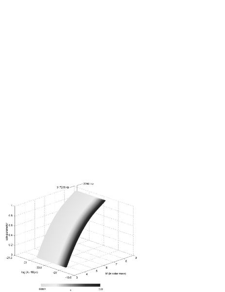
Figure 1: Volume formed by sets of parameters that correspond to frequencies varying from $f=3172.5\mathrm{Hz}$ to $3240\mathrm{Hz}$.

We obtain a certain volume in the space of parameters shown in figure 1 by fixing two boundary frequencies for the BH quadrupolar mode and then making those parameters to vary. Consequently any set of parameters inside that volume is within SCHENBERG bandwidth.

2 The simulated signal

We chose $\epsilon=0.01$, $M=4M_{\odot}$ and $\hat{a}=0.16$ to generate the signal that we used to calculate the signal-to-noise ratio. We believe that this efficiency is not overestimated since similar values have been found in the literature [3, 4].

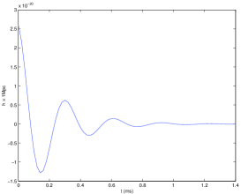
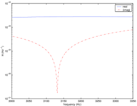
(a)	(b)

Figure 2: Waveform of a black hole ringdown (a) in the time domain and (b) in the frequency domain.

Figure 2.a shows the waveform $h(t)$ in the time domain. The Fourier transform of the impulse $h(t)$ is defined as

$$H(\omega)=\int_{-\infty}^{\infty}h(t)e^{-i\omega t}dt.$$ (4)

It represents the signal in the frequency domain and is shown in Figure 2.b. This figure shows that the signal spectrum on SCHENBERG bandwidth ($3.17-3.24\mathrm{kHz}$) is almost plane. This is a direct consequence of the low value for the BH’s quality factor ($Q\approx 2.16$, for that simulated signal). For higher values of the quality factor the damping function tends to a sinusoid and a peak may appear in the spectrum. This would facilitate the detection of the signal.

3 The SCHENBERG model

We modelled the SCHENBERG detector by assuming a linear elastic theory. Adopting this approach we determined the mechanical response of the system and obtained an expression for the case when six 2-mode mechanical resonators are coupled to the antenna’s surface according to the arrangement suggested by Johnson and Merkowitz, the truncated icosahedron configuration [5, 6]. We found an analytic expression to calculate the spectral density for the mode channels, given by [7]

$$S^{g}_{m}(\omega)=|\xi_{m}(\omega)|^{2}S^{\tilde{F}^{S}}_{m}+\sum_{j=1}^{6}|\Omega^{R_{1}}_{mj}(\omega)|^{2}S^{\tilde{F}^{N}_{R_{1}}}_{j}+\sum_{j=1}^{6}|\Omega^{R_{2}}_{mj}(\omega)|^{2}S^{\tilde{F}^{N}_{R_{2}}}_{j}.$$ (5)

The scalar $\xi_{m}(\omega)$ represents the transfer function of the sphere’s internal forces ${\tilde{F}^{S}}_{m}$ at angular frequency $\omega$ on mode $m$. The matrix elements $\Omega^{R_{i}}_{mj}(\omega)$ correspond to the response functions of channel $m$ to the noise forces $\tilde{F}^{N_{R_{i}}}_{j}$ that are acting on the mode $i$ of resonator $j$. $S^{X}$ denotes the spectral density of the quantity $X$. In order to find equation 5, we assumed that all noise sources and possible signals were statistically independent so the cross terms could be neglected.

The GW effective force [7, 8, 9] that acts on the sphere (in the frequency domain) has spectral density

$$S^{\tilde{\mathcal{F}}^{GW}}_{m}(\omega)=\left(\frac{1}{2}\omega^{2}m_{S}\chi R\right)^{2}S^{\tilde{h}}_{m}(\omega).$$ (6)

The sensitivity curve for mode $m$ is given through

$$\tilde{h}_{m}(\omega)=\sqrt{\frac{1}{\left(\frac{1}{2}\omega^{2}m_{S}\chi R\right)^{2}}\frac{S^{g}_{m}(\omega)}{|\xi_{m}(\omega)|^{2}}}.$$ (7)

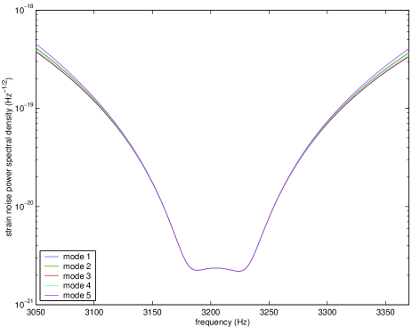
Figure 3: Sensitivity curve of SCHENBERG at $4.2\mathrm{K}$ for the quadrupolar normal modes $m$.

Figure 3 shows the sensitivity curves for the five quadrupolar normal modes of the sphere. We obtained this curve assuming that no signal was present and that only the usual noises in this kind of detector (Brownian noise, serial noise, back-action noise and electronic phase and amplitude noises) were disturbing the antenna at $4.2\mathrm{K}$. The absence of a signal made filtering unnecessary in this calculation. Also, we assumed a perfectly symmetric sphere, which implies identical transfer functions $\xi_{m}(\omega)$. Asymmetries on the sphere could make the transfer function of a mode different from the transfer function of the others.

4 Signal-to-noise ratio

Using the results in sections 2 (which inform about the signal) and 3 (which inform about the noise) it is easy to calculate the integrated signal-to-noise ratio ($SNR$). From the literature [10] we have

$$SNR=\frac{1}{2\pi}\int_{-\infty}^{+\infty}\frac{|H(\omega)|^{2}}{Sn(\omega)}d\omega.$$ (8)

The integral in equation 8, which is dominated by the interval of SCHENBERG bandwidth, gives $SNR\gtrsim 1$ for the simulated signal when the BH’s distance is $r\sim 20\mathrm{kpc}$.

5 Conclusion

If a low-spinning BH ($\hat{a}\sim 0.16$) with mass $\sim 4M_{\odot}$ and emission of about $1\%$ of its mass-energy in the form of GW exists up to a distance of $\sim 20\mathrm{kpc}$, then the SCHENBERG detector is expected to observe it when operating at $4.2\mathrm{K}$.

In the calculation we didn’t take into account other possible dependencies on the BH parameters except the known frequency-mass dependence. Strong dependencies between $\epsilon$ and $\hat{a}$ may make signals from high-spinning BHs much stronger.

There are theories that claim the existence of BHs but experimental evidences are indirect and inconclusive. Certainly it is not yet possible to predict the correct number of galactic BHs. However, the radius of $\sim 20\mathrm{kpc}$ includes the galactic center and the majority of the spiral arms, which are the most probable birthplaces for stellar BHs. So the detection of the kind of signal investigated in this work is an opportunity for gravitational wave astronomers to make essential discoveries about the black hole population in our galaxy.

References

References

- [1] F. Echeverria, Phys. Rev. D 40, 3194 (1989).
- [2] E. W. Leaver, Proc. R. Soc. London, Ser. A 402, 285 (1985).
- [3] J. D. E. Creighton, Phys. Rev. D 60, 022001-1 (1999).
- [4] J. D. E. Creighton, GRASP 1.9.8 - Users Manual, ed. B. Allen, p. 251 (1999).
- [5] W. W. Johnson and S. M. Merkowitz, Phys. Rev. Letters, 70, 2367 (1993).
- [6] S. M. Merkowitz and W. W. Johnson, Phys. Rev. D, 56, 7513 (1997).
- [7] C. A. Costa, O. D. Aguiar and N. S. Magalhães, (in preparation).
- [8] C. Z. Zhou, Phys. Rev. D, 51, 2517 (1995).
- [9] G. M. Harry, T. R. Stevenson and H. J. Paik, Phys. Rev. D, 54, 2409 (1996).
- [10] P. F. Michelson and R. C. Taber, J. Appl. Phys., 52, 4313 (1981).