Analysis of LIGO data for gravitational waves from binary neutron stars

Abstract

We report on a search for gravitational waves from coalescing compact binary systems in the Milky Way and the Magellanic Clouds. The analysis uses data taken by two of the three LIGO interferometers during the first LIGO science run and illustrates a method of setting upper limits on inspiral event rates using interferometer data. The analysis pipeline is described with particular attention to data selection and coincidence between the two interferometers. We establish an observational upper limit of $\mathcal{R}<\mbox{$1.7\times 10^{2}$}$ per year per Milky Way Equivalent Galaxy (MWEG), with $90\%$ confidence, on the coalescence rate of binary systems in which each component has a mass in the range $1$–$3$ $M_{\odot}$.

Currently at ]Stanford Linear Accelerator Center Currently at ]HP Laboratories Currently at ]Rutherford Appleton Laboratory Currently at ]University of California, Los Angeles Currently at ]Hofstra University Currently at ]Siemens AG Permanent Address: ]GReCO, Institut d’Astrophysique de Paris (CNRS) Currently at ]NASA Jet Propulsion Laboratory Currently at ]National Science Foundation Currently at ]University of Sheffield Currently at ]Ball Aerospace Corporation Currently at ]European Gravitational Observatory Currently at ]Intel Corp. Currently at ]Lightconnect Inc. Currently at ]Keck Observatory Currently at ]ESA Science and Technology Center Currently at ]Raytheon Corporation Currently at ]Mission Research Corporation Currently at ]Mission Research Corporation Currently at ]NASA Jet Propulsion Laboratory Currently at ]Harvard University Currently at ]Lockheed-Martin Corporation Currently at ]NASA Goddard Space Flight Center Permanent Address: ]University of Tokyo, Institute for Cosmic Ray Research Currently at ]Laboratoire d’Annecy-le-Vieux de Physique des Particules Permanent Address: ]University College Dublin Currently at ]Raytheon Corporation Currently at ]NASA Jet Propulsion Laboratory Currently at ]NASA Jet Propulsion Laboratory Currently at ]Research Electro-Optics Inc. Currently at ]Institute of Advanced Physics, Baton Rouge, LA Currently at ]Intel Corp. Currently at ]European Commission, DG Research, Brussels, Belgium Currently at ]Spectra Physics Corporation Currently at ]University of Chicago Currently at ]LightBit Corporation Currently at ]NASA Jet Propulsion Laboratory Currently at ]NASA Jet Propulsion Laboratory Currently at ]University of Delaware Currently at ]NASA Jet Propulsion Laboratory Currently at ]Carl Zeiss GmbH Currently at ]NASA Jet Propulsion Laboratory Currently at ]NASA Jet Propulsion Laboratory Currently at ]Shanghai Astronomical Observatory Currently at ]University of California, Los Angeles Currently at ]Laser Zentrum Hannover The LIGO Scientific Collaboration, http://www.ligo.org

I Introduction

The Laser Interferometer Gravitational-Wave Observatory (LIGO) is an ambitious US initiative to detect gravitational waves from astrophysical sources such as coalescing neutron stars and black holes, spinning neutron stars, and supernovae. The LIGO detectors are laser interferometers with light propagating between large suspended mirrors in two perpendicular arms. They measure the strain (differential fractional change in arm lengths) produced by gravitational waves from astrophysical sources by monitoring the relative optical phase between light paths in each arm Saulson (1994). LIGO comprises three detectors housed at two geographically distinct locations: in Hanford, WA, there are two interferometers, one with arms $4\,\text{km}$ long (which is referred to as H1 in this article) and one with arms $2\,\text{km}$ long (H2); in Livingston, LA there is one interferometer with arms $4\,\text{km}$ long (L1). The LIGO interferometers Abramovici et al. (1992); Barish and Weiss (1999) form part of a worldwide network of gravitational-wave detectors which includes the British-German GEO 600 detector Willke et al. (2002), the French-Italian VIRGO detector Acernese et al. (2002), the Japanese TAMA300 detector Tagoshi et al. (2001), and five resonant-bar detectors Allen et al. (2000).

Among the most likely sources of gravitational waves accessible to earth-based detectors are binary systems containing neutron stars and/or black holes Belczynski et al. (2002). When they reach design sensitivity, the initial interferometers in LIGO should be sensitive to gravitational waves generated during the last several minutes prior to coalescence. Current wisdom suggests that binary neutron star coalescences could provide up to $\sim 1/4$ events per year detectable by the initial LIGO interferometers at design sensitivity Kalogera et al. (2001); Cutler and Thorne (2001). Binary black hole coalescences could provide up to $\sim 2$ events per year Belczynski et al. (2002). The rates, however, are uncertain and may be significantly lower.

Previous published searches for gravitational waves from compact binaries used data from the LIGO 40m prototype Allen et al. (1999) and early data from the TAMA300 detector Tagoshi et al. (2001). The 40m data was taken in 1994 over a week-long run which yielded 25 hours of data and resulted in an upper limit rate of 0.5 events per hour in the Galaxy. The instrument was sensitive to sources up to 25 kpc away with signal-to-noise ratio equal to 10. The TAMA300 data was taken in 1999 over three nights which yielded 6 hours of data and resulted in an upper limit of 0.59 events per hour for events producing a signal-to-noise ratio larger than 7.2, corresponding to sources up to 6 kpc away. Searches for generic gravitational-wave bursts have also been performed using data from multiple detectors which operated simultaneously. Over 100 hours of data from prototype interferometers at Glasgow and Garching Nicholson et al. (1996), and four years of data from the International Gravitational Event Collaboration (IGEC) of resonant-bar detectors resulted in event rates consistent with the background of the instrumental noise Allen et al. (2000); Astone et al. (2003).

This article reports on the first search for gravitational waves from binary neutron star inspiral using LIGO data. The first scientific data run, called S1, lasted 17 days in 2002 and involved all three LIGO detectors. The detectors were sensitive to binary inspiral events to maximum distances (at signal-to-noise 8 in a single detector) between 30 and 180 kpc, depending on the instrument, allowing the most sensitive search yet. (The TAMA300 collaboration is currently analyzing $\sim 1000$ hours of data which will provide a comparable upper limit.) The GEO 600 detector Willke et al. (2002) collected data in coincidence with LIGO during the entire S1 run and achieved an excellent duty cycle of 98%. At the time of S1, GEO 600 was still being commissioned and was operated without signal recycling – an essential part of its final optical design. It was therefore operating at a sensitivity significantly lower than that of the LIGO detectors and its own target sensitivity. Hence GEO 600 was not included in this analysis. The upper limit reported here, $\mathcal{R}<\mbox{$1.7\times 10^{2}$}$ per year per Milky Way Equivalent Galaxy (MWEG), is the best direct observational limit on binary neutron-star coalescence to date. This rate is far from expected astrophysical rates, but demonstrates the progress of instrumental commissioning and success of the data analysis effort.

Many of the analysis techniques presented here will be used in future searches for gravitational waves. For instance, we expect to use these methods while analyzing data taken during the second LIGO science run between February and April 2003 when the detectors had roughly ten times better amplitude sensitivity than in S1.

The outline of the paper is as follows. Section II contains a description of the instruments, performance, sensitivity and duty cycle during S1. Section III describes in detail the target population of binary neutron-star systems and the gravitational waves they generate. The matched filtering technique used to search for these signals in the data is reviewed in Sec. IV. Filter outputs above a certain signal-to-noise ratio threshold constitute triggers which are cataloged for further analysis, provided they satisfy a $\chi^{2}$ test to determine the consistency of the data with the expected waveform. Section V describes data quality cuts and instrumental vetoes which are applied to eliminate triggers from times when the relevant interferometer was not operating properly. Surviving triggers are passed through an analysis pipeline which generates a list of event candidates from a combination of multi- and single-interferometer data, as detailed in Sec. VI. To avoid statistical bias, the veto conditions and pipeline parameters were tuned using a playground data set which was representative of, but separate from, the main data set. An upper limit on the rate of binary neutron star coalescences is calculated in Sec. VII, and systematic errors are considered in Sec. VIII. Section IX summarizes the results and discusses the prospects for future data runs.

II The LIGO Detectors

The LIGO interferometer design is a variant of a Michelson interferometer, with a laser light source and a beam splitter which directs the light along two perpendicular arms. Mirrors at the ends of the arms reflect the light beams back to the beam splitter, where they recombine and interfere according to their relative optical phase; this interference provides a sensitive measure of the length difference between the two arms. To augment the basic Michelson design, partially transmitting input mirrors are placed near the beam splitter to form a long Fabry-Perot cavity in each arm with a finesse of $\sim 220$. An additional partially transmitting mirror is placed in the path of the input laser beam to form a composite power-recycling cavity, which increases the amount of light circulating in the interferometer. A more detailed description of the LIGO optical configuration and other instrumentation may be found in Ref. Abbott et al. (2003).

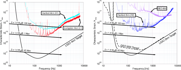
Figure 1: Typical sensitivities of the LIGO and GEO 600 interferometers during the S1 data run, shown as equivalent RMS strain amplitude spectral density $h_{\text{rms}}(f)=\sqrt{fS_{n}(f)}$, where $S_{n}(f)$ is the one-sided noise power spectral density. Typical noise spectra for the two 4km interferometers, L1 and H1, used in our analysis are shown in the left panel; the smooth solid curve indicates the target sensitivity of the LIGO 4 km interferometer design. Spectra for the 2km interferometer H2 and GEO 600 are shown in the right panel; the smooth solid and dashed curves indicates the target sensitivities of the LIGO 2 km and GEO 600 interferometer designs. The thick lines with arrowheads show the characteristic strains, $h_{\text{char}}(f)=f\tilde{h}(f)$, expected from binary neutron star systems (optimally located and oriented with respect to the detector) during the last few minutes before coalescence. These characteristic strains are approximately equal to the amplitude of a gravitational wave signal at a given frequency times the square-root of the number of cycles produced in a logarithmic band about the given frequency. The ratio of $h_{\text{char}}$ to $h_{\text{rms}}$ in the sensitive band of the instrument provides an estimate of the signal-to-noise ratio that could be achieved in detecting such a signal using matched filtering. When the LIGO instruments are operating at the target sensitivity, inspirals of double neutron stars ($2\times 1.4M_{\odot}$) are expected to be detectable within an equivalent volume $\approx(4\pi/3)\times(21\textrm{ Mpc})^{3}$.

The light source for each interferometer is a medium power Nd:YAG laser, operating at a wavelength of 1.06 $\mu$m Savage et al. (1998). Before the light is directed into the interferometer, its frequency, amplitude and direction are stabilized using a combination of active and passive stabilization techniques.

To isolate the mirrors and other elements from ground and acoustic vibrations, the detectors employ active and passive seismic isolation systems Giaime et al. (1996, 2003), from which the mirrors are suspended as pendulums. These form a coupled oscillator system with high isolation for frequencies above 40 Hz. The mirrors, major optical components, vibration isolation systems, and main optical paths are all enclosed in a high vacuum system.

Various feedback control systems are used to keep the multiple optical cavities tightly on resonance Fritschel et al. (2001) and well aligned Fritschel et al. (1998). The strain signal $s(t)=[L_{x}(t)-L_{y}(t)]/L$ is derived from the error signal of the feedback loop used to control the differential motion of the interferometer arms. To calibrate the error signal, the effect of the feedback loop gain is measured and divided out, and the response $R(f)$ to a differential arm strain is measured and factored in. The absolute scale of the response is established using the laser wavelength by measuring the mirror drive signal required to move through a given fraction of a fringe. The response varied over the course of the S1 run due to drifts in the alignment of the optical elements; it was tracked by injecting fixed-amplitude sinusoidal signals (calibration lines) into the differential arm control loop, and monitoring the amplitudes of these signals at the measurement (error) point Adhikari et al. (2003).

The interferometer noise is characterized by the one-sided power spectral density $S_{n}(f)$ of the signal $s(t)$. The sources of noise that are expected to limit the eventual sensitivity of the LIGO detectors are shot noise (determined by circulating light power, dominant at high frequencies), thermal noise (determined by energy dissipation mechanisms in the mirrors and suspensions, dominant at intermediate frequencies), and seismic noise (dominant at low frequencies). Figure 1 shows the expected noise due to these effects (at LIGO’s design target), expressed as RMS strain noise, along with typical spectra achieved by the LIGO interferometers during the S1 run. (Typical GEO 600 noise during S1 is also shown for comparison.) The differences among the three LIGO spectra reflect differences in the operating parameters and hardware implementations of the three instruments which are in various stages of reaching the final design configuration. For example, all interferometers operated during S1 at a substantially lower effective laser power level than the eventual level of 6 W at the interferometer input. Thus the shot-noise region of the spectrum, above 200 Hz, is much higher than the design goal. In addition, the S1 configuration only had a partial implementation of the laser frequency and amplitude stabilization systems, and a partial implementation of alignment control systems for the mirrors and the beam splitters. Despite these shortcomings, the detectors were sensitive to binary neutron star coalescences within the Galaxy and the Magellanic Clouds as illustrated in Fig. 2.

The 17-day run yielded 363 hours of data when at least one interferometer was in stable operation. The three interferometers were simultaneously in stable operation for 96 hours. For the analysis presented in this article, we chose to use data only from the two 4 km detectors, L1 and H1. While H2 was nearly as sensitive as H1, its noise exhibited a greater degree of non-stationarity, leading to a rate of spurious triggers which would have compromised the sensitivity of the search. L1 and H1 were simultaneously operational for 116 hours during the S1 run, providing data for the first combined analysis of interferometric detectors sensitive to inspiral events throughout the Galaxy. In addition, they were separately operational for 54 and 119 hours, respectively.

III Target population and Waveforms

Radio observations of pulsars confirm the existence of binary neutron star systems in the Galaxy Hulse (1994); Taylor (1994). General relativity predicts the decay of a binary orbit due to the emission of gravitational radiation. The decay rate inferred from observations of PSR1913+16 agrees with the prediction within 0.3% Taylor and Weisberg (1982, 1989); Weisberg and Taylor (2003). The orbital decay is easily modeled for compact binary systems containing neutron stars or stellar mass black holes. The binary orbit is expected to evolve through the LIGO frequency band by the emission of gravitational waves alone, making it possible to accurately compute the evolution without reference to complicated micro-physics.

When a compact binary system first forms, the orbit may be widely separated and highly eccentric. (See Ref. Belczynski et al. (2002) for a discussion and plots of birth separations and eccentricities). Gravitational radiation, emitted predominantly at twice the orbital frequency of the binary system, causes the orbit to shrink and circularize (much faster than it shrinks Peters (1964)) so that the binary components eventually spiral together along a sequence of nearly circular orbits with decreasing period. For binary neutron stars or stellar-mass black holes, the gravitational radiation eventually enters the frequency band of earth-based gravitational-wave detectors. At this point, the orbit decays rapidly and the gravitational waveform chirps upward in frequency and amplitude, sweeping through LIGO’s sensitive band. During S1, the LIGO interferometers were sensitive to gravitational-wave frequencies above about 100 Hz; an inspiral signal from two $1.4M_{\odot}$ objects would traverse the sensitive band in 2 seconds. At design sensitivity, the sensitive band will stretch down to $\simeq 40$ Hz and the signals will spend about 30 seconds in the sensitive band.

For low-mass binary systems, the waveforms are well approximated by a post-Newtonian expansion Blanchet et al. (1995, 1996); Damour et al. (2001) in the LIGO frequency band. Due to the uneven convergence of this expansion and a still indeterminate coefficient at higher order, we used second-order post-Newtonian waveforms Blanchet et al. (1996) in this analysis. The waveforms are parameterized by the masses of the two companions $I=(m_{1},m_{2})$, the inclination of the orbit relative to the plane of the sky, and the starting orbital phase. Other orbital parameters such as eccentricity and spin are not expected to be significant for binary neutron star coalescence Bildsten and Cutler (1992); Apostolatos (1995); Belczynski et al. (2002), so we do not consider them in this analysis. The strain produced in the instrument is written as

$$h(t)=\frac{1\textrm{ Mpc}}{D_{\mathrm{eff}}}\bigl{[}\sin\alpha\,h^{I}_{s}(t-t_{c})+\cos\alpha\,h^{I}_{c}(t-t_{c})]\;,$$ (1)

where $\alpha$ depends on the orbital phase and orientation of the binary system, $t_{c}$ is the time (at the detector) when the binary reaches its inner-most stable circular orbit, and $h^{I}_{s,c}(t-t_{c})$ are the two polarizations of the gravitational waveform produced by an inspiralling binary that is optimally oriented at a distance of 1 Mpc. An optimally-oriented binary system is one that lies on the detector’s $z$-axis with its orbital plane parallel to the $x$-$y$ plane, defined by the arms of the detector (i.e., directly above or below the detector and orbiting on the plane of the sky). The effective distance $D_{\mathrm{eff}}$ depends on the true distance $r$ to the binary, its location in the sky relative to the detector, and its orientation. This dependence is, in part, caused by the non-uniform detector response over the sky. If the source is not optimally oriented, then $D_{\mathrm{eff}}>r$. The binary inspiral waveform can thus be parameterized (for a single detector) in terms of the component masses, the effective distance, and the signal phase.

The rate at which neutron star binaries coalesce in our Galaxy can be estimated using the observed sample of binary pulsars. (See, for example, Ref. Kalogera et al. (2001).) This rate estimate can be extrapolated to extra-galactic distances (following Phinney Phinney (1991)) by assuming that the coalescence rate is proportional to the formation rate of massive stars and that the primordial binary population in our Galaxy is typical. Since the rate of massive star formation is proportional to blue-light (B-band) luminosity, the number of coalescences contributed by another galaxy is determined by the ratio of its blue-light luminosity to that of the Milky Way. The sample population for our analysis used spatial and mass distributions from a Milky Way population produced by the simulations of Ref. Belczynski et al. (2002) with the spatial distribution described in Ref. Kim et al. (2003). Additional sources from the Large and Small Magellanic Clouds, treated as points at their known distances and sky positions, were also added. The number of sources was proportional to the absolute blue-light luminosity of the LMC and SMC, with correction factors applied to account for reddening and the lower metallicity of these objects. The latter leads to lower neutron star formation rates primarily due to weaker stellar winds, which in turn favor the formation of more massive compact objects. With these corrections, the event rates from the Large and Small Magellanic Clouds are taken to be 11% and 2% of the Milky Way rate. We note that this population model may not be exactly accurate, but is representative of the current understanding of binary neutron star formation.

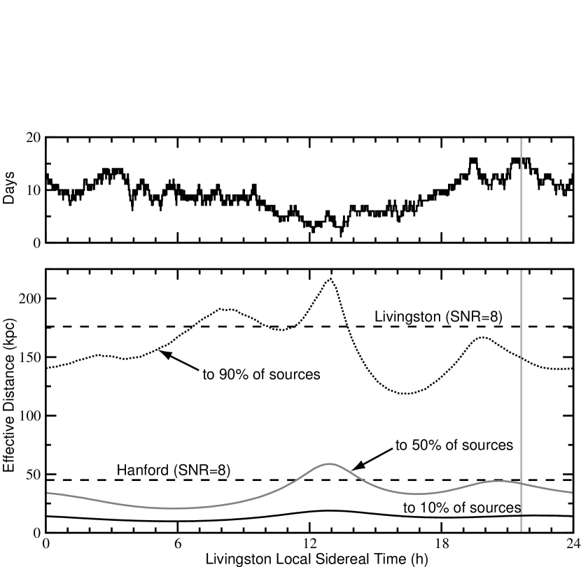
Figure 2: Summary of detector status and sensitivity to the population of neutron stars described in Sec. III as a function of sidereal time. For a given sidereal time, the upper panel shows the number of days during the run when at least one of the interferometers (H1 or L1) was collecting scientific data. For reference, the vertical dotted line indicates 05:00 UTC (corresponding to midnight at Livingston) on September 01, 2002. The lower panel shows the effective distance as measured in Livingston [and defined by Eq. (1)] to 10%, 50%, and 90% of the binary neutron star population described in Sec. III. The horizontal dashed lines show the average distance at which an inspiral of $2\times 1.4M_{\odot}$ neutron stars, in the optimal direction and orientation with respect to each detector, would produce a signal-to-noise ratio of 8, i.e. 176 kpc for L1 and 46 kpc for H1.

IV Template Based Trigger Generation

The data stream from each detector was searched for inspiral waveforms using matched filtering, i.e., by evaluating the correlation (with a frequency-dependent weighting to suppress noise) between the data and a template waveform for all possible coalescence times. We use templates for non-spinning binaries, so each waveform is identified by a mass pair $I=(m_{1},m_{2})$, a phase $\alpha$ and a distance $D_{\mathrm{eff}}$ as described above. The gravitational wave signals also obey the approximate relationship

$$\tilde{h}^{I}_{c}(f)=-i\tilde{h}^{I}_{s}(f)\;,$$ (2)

where $f>0$ and the Fourier transform $\tilde{q}(f)$ is defined by

$$\tilde{q}(f)=\int_{-\infty}^{\infty}e^{-2\pi ift}q(t)\,dt\;.$$ (3)

We exploit the symmetry (2), which is exact within the stationary-phase approximation used in this analysis, to reduce computational overhead in searching over the phase $\alpha$. If the detector’s calibrated strain data is $s(t)=n(t)+h(t)$, where $n(t)$ is the instrumental strain noise and $h(t)$ is a gravitational wave signal (if present), then the matched filter output for given masses $I=(m_{1},m_{2})$ is the complex time series

$$z(t)=x(t)+iy(t)=4\int_{0}^{\infty}\frac{\tilde{h}^{I}_{c}(f)\tilde{s}^{\ast}(f)}{S_{n}(f)}\,e^{2\pi ift}df$$ (4)

where $S_{n}(f)$ is the one-sided strain noise power spectral density. In this expression, $x(t)$ is the matched filter response to the $\alpha=0$ waveform $h^{I}_{c}$ while $y(t)$ is the matched filter response to the $\alpha=\pi/2$ waveform $h^{I}_{s}$. Matched filtering theory Wainstein and Zubakov (1962) provides a simple way to search over the phase $\alpha$: construct the signal-to-noise ratio (SNR) of the matched filter output,

$$\rho(t)=\frac{|z(t)|}{\sigma},$$ (5)

where

$$\sigma^{2}=4\int_{0}^{\infty}\frac{|\tilde{h}^{I}_{c}(f)|^{2}}{S_{n}(f)}df$$ (6)

is the variance of the matched filter output due to detector noise. For stationary and Gaussian noise, $\rho$ is the optimal detection statistic for a single detector.

The waveform (1) depends on the masses of the two companions, so a bank of templates that covers the expected range of neutron star masses must be used Owen and Sathyaprakash (1999). We adopted a template bank that covers the mass range $1\mbox{--}3\,M_{\odot}$ for each companion. The discrete bank was designed to cause less than $3\%$ loss in SNR due to parameter mismatches between any waveform and the nearest template in the bank. The layout of the template bank depends on the noise power spectral density of the instrument. A single template bank was used in this analysis: banks were first generated for each instrument and the bank with the most templates (in this case, the one generated for L1) was used. We checked that the resulting 2110 templates covered the mass range with $\leq 2\%$ loss of SNR for L1 and $\leq 7\%$ loss for H1. Waveforms with total mass below $4.0M_{\odot}$ incurred $\leq 3\%$ loss of SNR in both instruments. Using a single template bank allows easier comparison of inspiral candidates in the coincidence step of our analysis.

To reject transient noise artifacts that may excite a matched filter, but do not accumulate SNR as a chirp signal would, we employed an additional time-frequency veto in which the contribution to the filter output $z(t)$ from $p$ frequency sub-bands is compared to the expected contribution for the templates Allen et al. (1999); Allen (1998). The frequency sub-bands were chosen so that the expected chirp would produce an equal contribution to both the real and imaginary components of the filter output from each sub-band. The chirp for each sub-band is filtered to produce the $p$ complex-quantities $z_{l}(t)$ and the statistic is constructed as

$$\chi^{2}(t)=\frac{p}{\sigma^{2}}\sum_{l=1}^{p}|z_{l}(t)-z(t)/p|^{2}.$$ (7)

In the presence of Gaussian noise alone, $\chi^{2}$ is chi-squared distributed with $\nu=2p-2$ degrees of freedom. In this analysis, we did not optimize over different values of $p$, but chose $p=8$ which worked well.

If a putative signal $h(t)$ has masses which do not exactly match any template in the bank, then $\chi^{2}$ has a non-central chi-squared distribution with $2p-2$ degrees of freedom and a non-central parameter $\lambda=2\rho^{2}\varepsilon^{2}$, where $\rho$ is the SNR for the signal and $\varepsilon$ is the fractional loss of SNR due to parameter mismatch. While it is possible to construct constant confidence thresholds on the non-central chi-squared distribution for various signals, in this analysis we simply require

$$\chi^{2}<5(p+0.03\rho^{2})$$ (8)

for any inspiral event, where $p=8$ as described above. We refer to this cut as the $\chi^{2}$-veto. Since the detector noise was not Gaussian, the threshold was selected based on performance in the playground data set described in Sec. V and not using the exact result for the non-central chi-squared distribution.

We identify possible inspirals in a single detector (H1 or L1) by finding maxima of $\rho(t)$ above a certain threshold (chosen to be $\rho^{\ast}=6.5$ in this analysis), subject to the $\chi^{2}$-veto constraint of Eq. (8), and separated in time by at least the length of the template. Each such maximum is considered a trigger; the inferred coalescence time, $\rho$, and $\chi^{2}$ values are cataloged in a database along with the template parameters and effective distance (in Mpc), $D_{\text{eff}}=\sigma/\rho$.

Figure 3: Times when an interferometer was in stable operation were identified as science mode epochs indicated by the thick black lines at the top of the figure. These science mode epochs were analyzed in blocks of 256 seconds overlapped by 32 seconds (indicated in white). If there was not enough data at the end of a science mode epoch to take a 256 second block for analysis, the extra data was dropped from the analysis. Each of these blocks were further divided into 7 overlapping segments of 64 seconds which were then searched for inspiral signals. The overlaps are needed to avoid contamination in the correlation used to compute the SNR.

Times when each interferometer was in stable operation were identified as science mode epochs. These science mode epochs were analyzed in blocks of 256 seconds overlapped by 32 seconds as shown in Fig. 3. If there was not enough data at the end of a science mode epoch to take a 256 second block for analysis, the extra data was dropped from the analysis. Each 256 second block was read by the LIGO Data Analysis System (ldas) LDA , which down-sampled it from 16 kHz to 4 kHz. The power spectrum of the data was estimated for each block by dividing it into four 64 second segments and taking the mean power spectrum of these four segments. The matched filter given in Eq. (4) was implemented on 64 second data segments using routines in the LSC Algorithm Library (lal) LAL . In order to avoid end-effects in performing the correlation described by Eq. (4), we modified $1/S_{n}(f)$ so that its inverse Fourier transform had a maximum duration of $\pm$16 seconds. The first and last 16 seconds of each filtered 64 second segment were ignored as corrupted by the end-effects of the filter. The 64 second segments were overlapped by 32 seconds—thus forming 7 overlapping segments in each 256 second block—so that no data was lost within each block. Since the blocks were also overlapped by 32 seconds, only the first 16 seconds of data from the first block and the last 16 seconds of data from the last block were lost from each science-mode epoch. These effects combined result in the loss of 14 hours of data from each of the L1 and H1 interferometers.

When the interferometers at Hanford and Livingston were in stable operation, we checked for coincident signals to improve confidence in a detection. Since the Hanford and Livingston detectors are approximately co-aligned, they should observe essentially the same gravitational-wave signal. Ignoring mis-alignment and assuming the instrumental noise is Gaussian and uncorrelated, the optimal detection statistic can be written as

$$\rho^{2}_{\text{coherent}}(t)=\max_{\tau}\frac{|z_{\text{L1}}(t)+z_{\text{H1}}(t+\tau)|^{2}}{\sigma_{\text{L1}}^{2}+\sigma_{\text{H1}}^{2}}$$ (9)

where $z_{\text{L1}}(t)$ and $z_{\text{H1}}(t)$ are the complex matched filter outputs from the L1 and H1 detectors, $\sigma_{\text{L1}}^{2}$ and $\sigma_{\text{H1}}^{2}$ are the variances of these matched filter outputs for the two detectors, $\tau$ is the difference in the arrival time of the signal between the two detectors, and the maximization is performed over all possible values of $\tau$ up to the light-travel time between the two detectors ($\pm 10$ ms) Pai et al. (2001); Finn (2001a). This statistic uses the same template in each instrument and assumes that the time of arrival is consistent with the light travel time between the instruments. Since $\sigma$ [Eq. (6)] depends on the inverse power spectral density, a large value indicates good sensitivity. If, for example, L1 is considerably more sensitive than H1 (as it was during S1), then $\sigma_{\text{L1}}\gg\sigma_{\text{H1}}$. Thus, one has $|z_{\text{L1}}|\gg|z_{\text{H1}}|$ both during typical operation and when a signal is present, and a good approximation to the coherent statistic is

$$\rho^{2}_{\text{coherent}}\simeq|z_{\text{L1}}|^{2}/\sigma_{\text{L1}}^{2}=\rho_{\text{L1}}^{2}\;.$$ (10)

Since L1 was much more sensitive than H1 during the S1 run, $\rho_{\text{coherent}}$ for an event seen while both detectors were operating is well approximated by the $\rho$ value for L1 alone; when only H1 was operating, $\rho_{\text{coherent}}$ reduces to the $\rho$ value for H1 since the contributions from L1 vanish. We also note that a binary inspiral signal would have $\rho_{\text{L1}}\gtrsim 4\rho_{\text{H1}}$, so a genuine signal would not produce a trigger in H1 unless it appears in L1 with very high SNR (greater than $\sim 26$).

V Data Quality Criteria and Vetoes

The performance of the LIGO interferometers varied significantly during the S1 run on both long and short time scales. We omitted intervals of data from a given interferometer if it was not properly calibrated or if it had an unusually high level of noise, as described below. We also were able to veto some individual triggers which had a clear instrumental origin. To avoid statistical bias, the specific veto criteria were decided based on studies of a playground data set comprising roughly 10% of the data collected when all three interferometers were operating. This data was excluded from calculation of the final analysis results.

V.1 Instrumental calibration

As mentioned in Section II, the time variation of the interferometer response was tracked by continuously injecting sinusoidal signals with known amplitudes. The calibration was updated once per minute, and the analysis of each 256-second block of data used the first available calibration update within the block. There were periods of time when the sinusoidal injections were absent, however, and the calibration could not be updated. Blocks of data in which such a calibration drop-out occurred were not analyzed. There were also some periods of time when H1 calibration information was present but was deemed unreliable; these periods also were omitted from the analysis. In total, 17 hours of H1 data and 8 hours of L1 data were omitted from the analysis because of missing or unreliable calibration data.

V.2 Noise level

The noise in the gravitational-wave channel of each interferometer was sensitive to optical alignment, servo control settings, and environmental conditions. During most of the run, the noise level varied by less than a factor of two; however, there were a number of times when the noise level was significantly higher. We chose to omit these periods when the noise was particularly high. The specific criteria were developed by the working group searching for gravitational-wave bursts and adopted for the inspiral analysis as well. Each interferometer’s performance was tracked by calculating the band-limited root-mean-square noise (BLRMS) in four frequency bands $\{B_{1},B_{2},B_{3},B_{4}\}=${320–400 Hz, 400–600 Hz, 600–1600 Hz, 1600–3000 Hz}. For each band, the noise power $P_{i}(t)$ was calculated every $1/8$ seconds, then averaged over 360-second time intervals and compared to the mean value $\bar{P}_{i}$ for all science-mode data collected. Based on empirical studies of correlations between the power in each band and non-stationarity of the noise, we decided to eliminate any contiguous epoch of science data if there was any 360-second interval during the epoch for which $P_{1}>10\,\bar{P}_{1}$ or $P_{j}>3\,\bar{P}_{j}$ for $j=2,3,4$. This BLRMS cut removed 13 hours (8%) of the L1 data and 43 hours (18%) of the H1 data.

Since the BLRMS cut uses the noise in the gravitational-wave channel to identify times when data quality is suspect, a sufficiently strong inspiral signal could potentially cause the veto to be invoked. Based on the known amplitude response of the instruments, we determined that a binary neutron star inspiral signal would be vetoed in this way only if it were closer than $\sim 300$ pc, corresponding to a SNR of $4.7\times 10^{3}$ in L1. By way of confirmation, we also computed $P_{i}$ for periods when large-amplitude simulated inspiral waveforms were injected into the interferometers. The observed safety margin was consistent with the model calculations. Since $\ll 1\%$ of the target population is within 300 pc of Earth, the systematic effects of the BLRMS cut on our search were negligible.

V.3 Instrumental vetoes

The data quality cuts described above addressed performance variations over long time scales. Each of the interferometers also exhibited non-stationary behavior on short time scales, with occasional glitches and/or brief periods of elevated broadband noise in the gravitational-wave channel. Because the matched filtering technique used in this analysis assumed the noise spectrum to be stationary over periods of several minutes, these transients tended to excite the inspiral filter bank in such a way as to be recorded as triggers with fairly large SNR, even though they did not closely resemble the waveform of an inspiral. The $\chi^{2}$ veto [Eq. (8)] eliminated many of these triggers, but some remained, appearing as a high-side tail in the SNR distribution of inspiral triggers found in the playground data set.

We attempted to identify environmental or instrumental origins for these high-SNR triggers by checking for coincident transients in the many auxiliary data channels which were recorded along with the gravitational-wave channel. These included environmental monitoring sensors (seismometers, accelerometers, magnetometers, etc.) as well as various signals related to the operation of the interferometers. We evaluated several transient-detection algorithms, eventually choosing a simple one which applies a high-pass filter to the data and records excursions from zero which exceed a given size threshold. We developed an automated procedure to veto any inspiral trigger within a given time window around auxiliary-channel glitches found by this algorithm. For each of several promising auxiliary channels, the excursion size threshold and time window were tuned using the playground data set to maximize the number of triggers vetoed without introducing undue dead-time. The results of these studies for each interferometer are summarized below.

The H1 detector experienced distinct glitches in the gravitational-wave channel at a rate of about 4 per hour. Although no external environmental cause was identified, nearly all of these glitches were clearly visible in an auxiliary channel derived from a photo-diode at the interferometer’s reflected port. This channel is sensitive to the average arm length and is used to control the frequency of the laser light. We vetoed inspiral triggers within a $\pm 1$ second window on either side of glitches found in this auxiliary channel; this veto condition introduced a dead-time of 0.2%. Based on the detector design, a real gravitational wave would not be expected to appear with a significant amplitude in this auxiliary channel; we verified this experimentally by injecting simulated inspiral waveforms into the interferometer arm length control servo (changing the arm lengths using electromagnetic actuation to push the suspended mirrors) and observing the signal strength in this and other auxiliary channels.

High-SNR inspiral triggers in the L1 detector were strongly correlated with transients in an auxiliary channel derived from the photo-diode at the interferometer’s antisymmetric port, nominally orthogonal in demodulation phase relative to the gravitational-wave channel. This auxiliary channel was not used to control any degree of freedom in the interferometer; it was sensitive to imbalance in the modulation sidebands and to alignment fluctuations. This suggested its use as a veto channel. Unfortunately, simulated inspiral waveforms injected into the arm length control servo appeared with non-negligible amplitude in this auxiliary channel. We suspect this was an artifact of injecting a large signal with imperfectly balanced mirror actuators, introducing an oscillatory misalignment. To be safe, however, we chose not to veto based on this channel. No other auxiliary channel offered an efficient veto, so no instrumental veto was applied for L1.

VI Analysis Pipeline and Tuning

The detection of a gravitational-wave inspiral signal in the S1 data would (at the least) require triggers in both L1 and H1 with consistent arrival times (separated by less than the light travel time between the detectors) and waveform parameters. Such a temporal coincidence requirement has the advantage of greatly reducing the background rate due to spurious triggers in the individual detectors. It limits the volume of space searched to that which can be seen by the less sensitive detector, however, and it limits the observation time to the periods of simultaneous operation. Because the L1 detector was much more sensitive than H1 during the S1 run, and because they operated simultaneously less than $30\%$ of the time, we developed a more sophisticated (upper-limit) analysis pipeline which makes use of triggers from the individual detectors when a coincidence test is not possible. Studies of the playground data set indicated that the additional background rate introduced by this choice should not offset the improvement in event rate limit that comes from increased observation time. Of course, event candidates identified during non-coincident observation times could not lead to an unambiguous detection of gravitational waves.

Our analysis pipeline is summarized in Fig. 4. We follow five steps to produce a list of non-vetoed event candidates which represent the background due to detector noise (plus any gravitational-wave signals, if present) during periods of nominal operation. (1) Analyze the gravitational-wave channel data from each detector using matched filtering as described above. When $\rho>6.5$ in an individual detector, apply the $\chi^{2}$ veto to eliminate spurious excitations of the templates. Store information about the surviving triggers in a database. (2) Apply the BLRMS cut to reject triggers in periods with unusually high noise, and apply a veto to eliminate H1 triggers with a clear instrumental origin. (3) When both interferometers are operating, require coincident triggers only if the effective distance measured by the L1 detector is closer than a cut-off distance $D^{\ast}$. (The selection of $D^{\ast}$ and the coincidence criteria is described below.) In this case, the SNR for the event candidate is taken to be the L1 SNR in accordance with the discussion around Eq. (10). If an L1 trigger has $D_{\mathrm{eff}}>D^{\ast}$, keep the trigger regardless of whether it was also detected by H1. (4) During times when only one interferometer is operating, keep any trigger that passes the cuts in the second step. (5) Finally, maximize all surviving triggers over time and over the template bank. The timing resolution of inspiral signals is $\lesssim 1$ ms once coincidence of template mass parameters in both instruments is enforced. When coincidence is unavailable, background noise can trigger many templates at significantly different times. Since the impulse response of the matched filter is $\sim 16$ seconds [because the template is effectively convolved with the frequency dependent weighting $1/S_{n}(f)$ when computing the SNR in Eq. 4], we maximize over all triggers in a $16$ second window and over the entire template bank to produce the final list of candidate events. The post-processing analysis described by steps (2)–(5) was performed using software in the package lalapps LAL .

We characterized our analysis pipeline using a Monte Carlo method in which we re-analyzed the data with simulated inspiral signals injected into the time series. The re-analysis used exactly the same pipeline as the original analysis and the simulated signals were drawn from the population described in Sec. III. The efficiency of the pipeline is the fraction of this population that could be detected. To avoid statistical bias, we used only the playground data set described in Sec. V when deciding aspects of the pipeline.

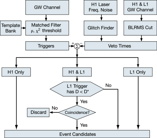
Figure 4: The inspiral analysis pipeline used to determine the reported upper limit. “H1 Only”, “H1 & L1”, and “L1 Only” indicate which interferometer(s) was/were operating when a trigger was recorded. This method of recording candidate events even when coincidence is not available allows a tighter bound to be placed on the rate of binary neutron star inspirals by providing more observation time and allowing for the much greater sensitivity of L1 than H1.

The coincident event selection criteria in step (3) were tuned by studying the fractional loss of efficiency of the pipeline. A trigger from H1 was considered coincident with a trigger from L1 if the recorded coalescence times were within a time window $\Delta t^{*}=0.011\mbox{ s}$. This accounts for the light travel time between the two sites (which is $0.010\mbox{ s}$) plus statistical and systematic errors in the individual measurements of coalescence time. The gross frequency evolution of an inspiral chirp signal is controlled by the chirp mass ${\mathcal{M}}=m_{1}^{3/5}m_{2}^{3/5}(m_{1}+m_{2})^{-1/5}$. The difference of chirp mass $\Delta{\mathcal{M}}=\mathcal{M}_{\text{L1}}-\mathcal{M}_{\text{H1}}$ for a pair of coincident (in time) triggers was required to satisfy $|\Delta{\mathcal{M}}|/\mathcal{M}_{\text{L1}}<10^{-2}$ leading to $\sim 1\%$ fractional loss of efficiency for the playground data. Finally, we chose $D^{\ast}=51$ kpc, producing $\sim 10\%$ fractional loss of efficiency for the playground data, in order to have a reasonable chance of detection in coincidence between the two sites.

VII Results from S1 data

The non-playground data was analyzed using the pipeline described above. After the division of the data into 256-second blocks, the rejection of blocks without reliable calibration, the additional loss of 16 seconds from the beginning of the first block and the end of the last block of a science-mode epoch, and the times during which a veto was active were discarded, a total of 236 hours of non-playground data remained: 58 hours when both L1 and H1 were operating, 76 hours when only L1 was operating, and 102 hours when only H1 was operating.

VII.1 Triggers and Event candidates

The triggers from each interferometer satisfy $\rho_{\text{coherent}}>6.5$ and the $\chi^{2}$ veto defined in Eq. (8). There were $\sim 2\times 10^{6}$ triggers from each detector before applying vetoes, checking for coincidence, and maximizing over templates and time with a 16 second window. The numbers of event candidates from each part of our pipeline with $\rho_{\text{coherent}}>8.0$ in the S1 data are summarized in Table 1.

Table 1: Number of event candidates with $\rho_{\text{coherent}}>8.0$ found via each of the pipeline paths shown in Fig. 4. The first two lines represent event candidates found while both interferometers were operating. No coincident events were detected in both interferometers; however, there were many event candidates found in L1 with effective distances $D_{\mathrm{eff}}>51\textrm{ kpc}$, which would not be detectable in H1 and thus are kept as event candidates. The last two lines represent event candidates found while only one interferometer was operating.

Operating	Detected in	Number	Max SNR
L1 and H1	L1 ($D_{\text{eff}}<51$ kpc) and H1	0	–
L1 and H1	L1 ($D_{\text{eff}}>51$ kpc)	418	15.6
L1 only	L1	786	15.9
H1 only	H1	274	12.0

No event candidates were found in coincidence by both detectors. If there had been one or more coincident event candidates, the background rate of accidental coincidences could have been determined from the data by counting coincidences after shifting the H1 trigger times relative to the L1 trigger times by an amount greater than the light travel time between the sites. In fact, in the S1 data, there were no triggers whatsoever in L1 which were close enough ($D_{\mathrm{eff}}<51\textrm{ kpc}$) to have been seen in H1 with $\rho_{\mathrm{H1}}>6.5$.

For comparison, Table 2${}^{\,\textrm{\footnotesize\ref{tablenote}}}$ shows the number of events identified with $\rho_{\text{coherent}}>8.0$ by the same analysis pipeline upon processing the output of the Monte-Carlo simulation described in Sec. VI. A total of 5071 simulated signals were overlaid on the S1 data, of which 619 were found in coincidence, demonstrating that the pipeline could correctly identify coincident event candidates within $51\textrm{ kpc}$. Note that the counts of event candidates in the other three paths of Table 2 include those in the underlying data, not associated with an injected signal.

Table 2: Results from the Monte-Carlo simulation given for comparison with the equivalent results of the search. Note that 619 simulated events were detected in coincidence, demonstrating that the pipeline was indeed capable of identifying coincident event candidates.

Operating	Detected in	Number	Max SNR
L1 and H1	L1 ($D_{\text{eff}}<51$ kpc) and H1	619	634.4
L1 and H1	L1 ($D_{\text{eff}}>51$ kpc)	773	46.5
L1 only	L1	2052	460.2
H1 only	H1	1623	221.9

Table 3: The five candidates with the largest SNR which remain at the end of the pipeline. This table indicates the time they registered in the detectors, the SNR, the value of $\chi^{2}$ per degree of freedom, the effective distance to an astrophysical event with the same parameters, and the binary component masses of the best matching template.

Date	UTC	GPS Time	Operating	Detected in	SNR	$\chi^{2}/\text{d.o.f.}$	$D_{\mathrm{eff}}$ (kpc)	$m_{1}$ ($M_{\odot}$)	$m_{2}$ ($M_{\odot}$)
2002/09/02	00:38:33.557	714962326.557	L1 only	L1	15.9	4.3	95.0	1.31	1.07
2002/09/08	12:31:38.282	715523511.282	L1 and H1	L1 ($D_{\text{eff}}>51$ kpc)	15.6	4.1	68.4	1.95	0.92
2002/08/25	13:33:31.000	714317624.000	L1 only	L1	15.3	4.9	100.7	3.28	1.16
2002/08/25	13:29:24.250	714317377.250	L1 only	L1	14.9	4.6	88.7	1.99	1.99
2002/09/02	13:06:56.731	715007229.731	L1 only	L1	13.7	2.2	96.3	1.38	1.38

The ten event candidates with the largest SNR in the pipeline were all detected by L1 and had SNR between 12 and 16 and $\chi^{2}$ per degree of freedom between 2.2 and 4.9. Details of the five largest events are given in Table 3. Four of these events have $\chi^{2}$ values close to the threshold in Eq. (8); the exception is the candidate which occurred at 13:06:56.731 UTC on 2002/09/02. Figure 5 (left panels) shows the signal-to-noise and $\chi^{2}$ time series for the candidate with the largest SNR, which occurred at 00:38:33.557 UTC on 2002/09/02. A simulated inspiral signal with comparable SNR is shown in Fig. 5 (right panels) to demonstrate the qualitative differences in the time series. Unlike the simulated signal, the SNR of the event candidate is consistently high across the duration of the event, with the value of the $\chi^{2}$ veto varying significantly and dropping below the threshold right at the time of maximum SNR.

Further scrutiny of the five largest SNR events revealed some instrumental problems. The event at 00:38:33.557 UTC on 2002/09/02 coincides in time with saturation of the photo-diode at the antisymmetric port. This saturation, which started a second before the recorded coalescence time for the candidate event and lasted several seconds, was likely due to an instrumental misalignment. The misalignment is indicated by a five-fold increase in the power at the dark port of the interferometer, starting three seconds before the coalescence time and lasting six seconds. This event would have been vetoed by the auxiliary-channel veto condition we considered for L1 but decided not to use (as discussed in Sec. V.3). The event recorded at 13:06:56.731 UTC on 2002/09/02 occurred when the interferometer was kept functioning during the most severe seismic conditions for S1 data. Another event candidate, with SNR $13.0$, occurred just 98 seconds later. The interferometer was rarely locked with seismic noise this high, and was probably experiencing up-conversion of low-frequency seismic noise into the gravitational-wave band through coupling with mechanical resonances and power line harmonics.

Event candidates detected in just one interferometer cannot be taken to be real gravitational wave inspirals with any confidence, since we do not understand the distribution of background. However, we can still place an upper limit on the rate of inspirals. Despite being able to find a posteriori reasons to justify eliminating some of the largest SNR event candidates as instrumental effects, we chose to keep them as event candidates for purposes of calculating the upper limit.

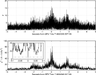
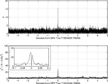
Figure 5: Left Panels: The largest SNR candidate event seen during our search of the LIGO data. This candidate event occurred at a time when only L1 was in stable operation. The top panel shows the signal-to-noise time series, $\rho(t)$. Notice that $\rho(t)>6.5$ many times in a $\sim 5$ second interval around the candidate event. The center panel shows $\chi^{2}/(p+0.03\rho^{2})$ as a function of time; notice $\chi^{2}/(p+0.03\rho^{2})>5$ for $\sim 5$ seconds around the candidate event, but drops below this threshold right at the time of maximum $\rho$. The inset shows this more clearly for $\pm 0.1$ second around the event where the threshold is indicated by a dot-dashed horizontal line. The bottom panel shows the time series for this candidate event after applying a high-pass filter with a knee frequency of 200 Hz. Notice the bursting behavior which does not look like an inspiral chirp signal. Right Panels: A simulated injection into the L1 data. This example was chosen for comparison with the largest SNR event shown in the left panels since it similar in mass parameters, detected signal to noise and $\chi^{2}$. The instrument was behaving well at the time around the simulated injection. The top panel shows that $\rho(t)<6.5$ except in close proximity to the signal detection time. The center panel shows $\chi^{2}/(p+0.03\rho^{2})$ as a function of time. Notice that it is much closer to threshold at all times around the simulated injection; this contrasts dramatically with the case of the candidate event shown in the left panels. The inset shows this more clearly for $\pm 0.1$ seconds around the injection. The bottom panel shows the time series for this simulated injection after applying a high-pass filter with a knee frequency of 200 Hz. The inspiral chirp signal is not visible in the noisy detector output.

VII.2 Upper Limit Analysis

To determine an upper limit on the rate of binary neutron star inspirals, we compare the observed distribution of events as a function of $\rho_{\text{coherent}}$ to the expected background plus the population of interest. The comparison is made based on criteria established in advance of the analysis. Typically, one might choose an SNR threshold $\rho^{\ast}$ based on the rate and distribution of background events and compare the number of observed events with $\rho>\rho^{\ast}$ to the expected background. Unfortunately, we have no model for the background events in each of the interferometers; this is problematic because we chose to include event candidates found in only one interferometer to increase the visible distance and observation time. Rather than choosing a fixed value for $\rho^{\ast}$, we adopt an approach in which $\rho^{\ast}$ is determined by the data. Specifically, we set $\rho^{\ast}$ equal to the largest SNR observed in the data and calculate the efficiency of the pipeline accordingly. Since no events are observed with $\rho>\rho^{\ast}$, we calculate an upper limit on the event rate for the modeled population assuming the probability of a background event above this SNR is negligibly small. This approach has the advantage of dealing with the lack of a model for the background events in a controlled manner.

If the population of sources produces Poisson-distributed events with a rate $\mathcal{R}$, the efficiency $\epsilon(\rho^{\ast})$ is also the probability that any given binary neutron star inspiral in the target population would have SNR greater than $\rho^{\ast}$. Then the probability of observing an inspiral signal with $\rho>\rho^{\ast}$, given some rate $\mathcal{R}$ and some observation time $T$, is

$$P(\rho>\rho^{\ast};{\mathcal{R}})=1-e^{-{\mathcal{R}}T\epsilon(\rho^{\ast})}.$$ (11)

A frequentist upper limit with $90\%$ confidence on the value of $\mathcal{R}$ is determined by solving $P(\rho>\rho_{\text{max}};{\mathcal{R}}_{90\%})=0.9$ for ${\mathcal{R}}_{90\%}$ where $\rho_{\text{max}}$ is the largest SNR event observed in the S1 data. The result can be written in closed form as

$${\mathcal{R}}_{90\%}=\frac{2.303}{T\epsilon_{\text{max}}}$$ (12)

where $\epsilon_{\text{max}}=\epsilon(\rho_{\text{max}})$ and $T$ is the observation time. For ${\mathcal{R}}>{\mathcal{R}}_{90\%}$, there is more than $90\%$ probability that at least one true inspiral event would be observed with SNR greater than $\rho_{\text{max}}$. This limit is conservative since the non-zero probability that a background event could have SNR greater than $\rho_{\text{max}}$ has been neglected.

It is useful to express the limit as a rate per Milky-Way Equivalent Galaxy (MWEG) for easy comparison with theoretical predictions and other observational results. The effective number of Milky Way equivalent galaxies to which the search was sensitive is

$$N_{\text{G}}=\epsilon_{\text{max}}\left(\frac{L_{\text{pop}}}{L_{\text{G}}}\right)$$ (13)

where $L_{\text{G}}=9\times 10^{9}L_{\odot}$ is the effective blue-light luminosity of the Milky Way and $L_{\text{pop}}$ is the effective blue-light luminosity of the population. The rate limit can be written as

$${\mathcal{R}}_{90\%}={2.303}\times\left(\frac{1\text{ y}}{T}\right)\left(\frac{1}{N_{\text{G}}}\right)\text{ y}^{-1}\text{ MWEG}^{-1}\;.$$ (14)

During the $T=236\text{ h}=0.027\text{ y}$ of data used in our analysis, the largest observed SNR was $\rho_{\text{max}}=15.9$. The detection efficiency was computed using a Monte Carlo simulation in which we re-analyzed the data with simulated inspiral signals, drawn from the population described in Sec. III, injected into the time series. The efficiency $\epsilon(\rho^{\ast})$, shown in Fig. 6(b), is the fraction of the 5071 simulated signals which were detected with $\rho>\rho^{\ast}$. The efficiency at $\rho^{\ast}=15.9$ is $\epsilon_{\text{max}}=0.53$. Folding this together with $L_{\text{pop}}=1.13L_{\text{G}}$, the nominal value of $N_{\text{G}}$ is $0.60$; however, this is subject to some uncertainties, to be discussed in the next section. As a function of the true value of $N_{\text{G}}$, the rate limit is

$${\mathcal{R}}_{90\%}=\mbox{$1.4\times 10^{2}$}\left(\frac{0.60}{N_{\text{G}}}\right)\text{ y}^{-1}\text{ MWEG}^{-1}\;.$$ (15)

It is interesting to compare our result with a direct estimate based on average sensitivity of the instruments (as shown in Fig. 2), properties of the population, and the observation times used in this analysis. At SNR $15.9$, L1 was sensitive to $80\%$ of the sources and H1 was sensitive to $35\%$ of sources in our model population. Out of 236 hours, L1 was the best detector for 134 hours and H1 for 102 hours. The expected efficiency is then

$$\epsilon(15.9)=(102\times 0.35+134\times 0.80)/236=0.6\;.$$ (16)

The measured efficiency is $\epsilon(15.9)=0.53$, but the $\chi^{2}$ veto and coincidence requirements both introduce some loss; the expectation based on playground data was $\approx 0.06\times 58/236=0.015$ decrease in efficiency from coincidence and a loss of about $\approx 0.06$ from the $\chi^{2}$. The actual loss from coincidence is $\approx 0.02$ as measured on the full data set. Consequently, the measured efficiency and hence the upper limit agree well with expectations.

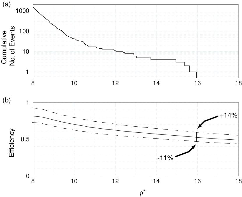
Figure 6: Panel (a) shows the number of events in the data with $\text{SNR}>\rho^{\ast}$ as a function of $\rho^{\ast}$. The largest event has $\text{SNR}=15.9$. Panel (b) shows the detection efficiency $\epsilon(\rho^{\ast})$ for sources in the target population (Milky Way and Magellanic Clouds) as a function of $\rho^{\ast}$. The dashed lines indicate boundaries of our estimated systematic errors on the efficiency.

VIII Error analysis

The interpretation of this search for gravitational waves from binary neutron star inspiral suffers from a number of systematic effects which could modify the upper limit. We classify these effects into three different types: (i) uncertainties in the population model and theoretical expectations about the sources; (ii) uncertainties in the instrumental calibration; (iii) deficiencies of the analysis pipeline. Each one can have a direct effect on the efficiency of the search to detect gravitational waves from the target population as it exists in nature.

VIII.1 Uncertainties in population model

Uncertainties in the population model used for the Monte-Carlo simulations may lead to differences between the inferred rate and the rate in the universe. Since the effective blue-light luminosity $L_{\text{pop}}$ is normalized to our Galaxy, variations arise from the relative contributions of other galaxies in the population. These contributions depend on the estimated distances to the galaxies, estimated reddening, and corrections for metallicity (lower values tend to produce higher mass binaries), among other things. Since the Magellanic Clouds contribute only $\sim 13\%$ of the blue light luminosity in this analysis, a conservative estimate of the uncertainties gives $L_{\text{pop}}=1.13\pm 0.06$.

The spatial distribution of the sources can also introduce significant uncertainties. Typically, the distances to nearby galaxies are only known to about 10% accuracy. Uncertainties in distances to galaxies near the limit of detector sensitivity are most relevant. As the detector sensitivity improves, more galaxies will be in this category, so it may become a major source of systematic uncertainty. It is not important for the current analysis, since the detectors were sensitive to the majority of sources in the Milky Way and Magellanic Clouds.

The effects of spin were ignored both in the population and in the waveforms used to detect inspiral signals. Apostolatos Apostolatos (1995) has performed the most complete analysis of the effects of spin on detection of waves from neutron star inspiral. His investigations suggest that less than $10\%$ of all possible spin orientations cause more than $\sim 5\%$ reduction in SNR for binary neutron star systems. There is insufficient information about the distribution of binary spin orientations to quantitatively estimate the systematic effect, but it seems certain that the fraction of the population with spin configurations which would interfere with their detection is negligible.

Different models for NS-NS formation can lead to small variations in the tails of the NS mass distribution Belczynski et al. (2002), but the bulk of the distribution always remains strongly peaked around observed NS masses Thorsett and Chakrabarty (1999). Since the detection efficiency depends most sensitively on the bulk properties of the mass distribution, the expected variations are negligible compared to other systematic effects discussed in this section.

VIII.2 Uncertainties in the instrumental response

The instrument response $R(f)$ was constructed for every minute of data during S1 from a reference sensing function $C(f)$, a reference open loop gain function $G(f)$, and a parameter $\alpha(t)$ representing varying optical gain Adhikari et al. (2003). The parameter $\alpha$ was reconstructed using the observed amplitudes of the calibration lines described in Section II. If an inspiral signal is present in the data, systematic errors in the calibration can cause a mismatch between the template and the signal. For simulated injections, the SNR differs from the SNR that would be recorded for a signal from a real inspiral event at the same distance as the injection. The effect is linear in amplitude errors causing either an upward or downward shift in SNR, but quadratic in phase errors causing an over-estimation of sensitivity. This effect is captured by shifting the efficiency curve in Fig. 6 horizontally by the appropriate amount.

A careful evaluation of uncertainties in the S1 calibration Adhikari et al. (2003) has shown that amplitude errors are primarily due to statistical fluctuations in the measurement procedure, while phase errors are mostly systematic and are greater at higher frequencies. Combining statistical and systematic errors in quadrature, the amplitude errors lead to $\sim 18\%$ errors in SNR in L1 and $\sim 8\%$ errors in H1. The phase errors lead to overestimation of the SNR by $\sim 2\%$ in L1 and $\sim 4\%$ in H1. Combining amplitude and phase errors in quadrature and taking the larger L1 values as representative, we find $\sim 18\%$ errors in SNR of Monte-Carlo injections which translates to fractional errors in efficiency $\sim\mbox{$+$14\%$/$$-$10\%}$, i.e. $\epsilon_{\text{max}}=0.53^{+0.07}_{-0.05}$.

To verify the data analysis methods, a few special studies were done in which simulated inspiral waveforms were injected into the interferometer hardware using the mirror actuators. We then used the analysis pipeline described above to recover the known mass and distance parameters of the injected signal. A side benefit of these injections is to build confidence in our understanding of calibration uncertainties. In order to simplify the analysis pipeline, the template bank was reduced to a single template, a $1.4,1.4\,M_{\odot}$ or a $4.0,1.4\,M_{\odot}$ inspiral, corresponding to the mass parameters of the injected signal. Unfortunately, the calibration signal was turned off during the injections, so we defined a set of possible response functions for this range, and studied the variation in the detected inspiral signal. This was possible because the parameter $\alpha$ has only a limited physical range. We found that the variation in the reconstructed signal to noise and effective distance was in agreement with our expectations. Since the parameter $\alpha$ has a known dependence on the interferometer alignment we were able to use auxiliary channel information to estimate its value during the injections. For this value the detected coalescence time of the chirp was the same as the injected time to within $1/4096$ seconds, i.e. one sample of filtered data, and the reconstructed distance and the injected distance agreed to within 12%, which is consistent with the errors quoted above.

VIII.3 Uncertainties in the analysis pipeline

Since we use matched filtering to search for gravitational waves from inspiralling binaries, differences between the theoretical and the real waveforms could also adversely effect the results. These effects have been studied in great detail for binary neutron star systems Apostolatos (1995); Droz and Poisson (1997); Droz (1999). The results indicate $\sim 10\%$ loss of SNR due to inaccurate modelling of the waveforms for binaries in the mass range of interest. This feeds into our result through our measurement of the efficiency. We may be over-estimating our sensitivity to real binary inspiral signals; this would shift all points on the efficiency curve in Fig. 6 to the left by $\sim 10\%$. This corresponds to fractional errors $\sim\mbox{$+$0\%$/$$-$5\%}$ in efficiency, i.e. $\epsilon_{\text{max}}=0.53^{+0.0}_{-0.03}$.

The effects of discreteness of the template placement, errors in the estimates of the power spectral density $S_{n}(f)$ used in the matched filter in Eq. (4), and trends in the instrumental noise are all accounted for by the Monte-Carlo simulation.

VIII.4 Combined uncertainties on $N_{\text{G}}$ and the rate

The efficiency incurs fractional errors $\sim\mbox{$+$14\%$/$$-$10\%}$ from calibration uncertainties (Sec. VIII.2) and $\sim\mbox{$+$0\%$/$$-$5\%}$ from inaccurate knowledge of the inspiral waveforms (Sec. VIII.3). Combining these in quadrature yields total errors $\sim\mbox{$+$14\%$/$$-$11\%}$ in the efficiency $\epsilon_{\text{max}}$. Adding these (not in quadrature) to the $\pm 5\%$ error for $L_{\text{pop}}$ (Sec VIII.1) yields

$$N_{\text{G}}=0.60^{+0.12}_{-0.10}\;.$$ (17)

To be conservative, we assume the downward excursion $N_{\text{G}}=0.60-0.10=0.50$ when using Eq. (15) to derive an observational upper limit on the rate of binary neutron star coalescence:

$${\mathcal{R}}<\mbox{$1.7\times 10^{2}$}\text{ y}^{-1}\text{ MWEG}^{-1}\;.$$ (18)

IX Conclusions and future directions

The first search for gravitational-wave signals from coalescing neutron stars in LIGO science data yielded no coincident event candidates. An observational upper limit $\mbox{$1.7\times 10^{2}$}\text{ y}^{-1}\text{ MWEG}^{-1}$ on the rate of neutron star inspirals was derived. This limit is better than previous direct limits by a factor of 26 Allen et al. (1999); Tagoshi et al. (2001).

Over the next few years, the sensitivity of the LIGO interferometers will be dramatically improved, to the point where inspirals of double neutron stars ($2\times 1.4M_{\odot}$) are expected to be detectable within an equivalent volume $\approx(4\pi/3)\times(21\textrm{ Mpc})^{3}$ Finn (2001b). Due to the non-uniform response of the detectors, this implies that a neutron star inspiral could be detected out to a maximum distance $\approx 46\textrm{ Mpc}$ if the binary is located directly above or below the detectors and orbits in the plane of the sky. The rate of coalescence of extra-galactic neutron star binaries is thought to be proportional to the rate of massive star formation which is, in turn, proportional to the blue light luminosity. (See, for example, Ref. Kalogera et al. (2001).) Using current galaxy catalogs, it is estimated that $N_{\text{G}}\approx 465$ MWEG will be detectable by LIGO (using the three detectors combined to produce a network SNR $>8$) Nutzman et al. (2003). If the coalescence rate of binary systems (in which each component has a mass in the range $1$–$3$ $M_{\odot}$) were as high as $\sim 5\times 10^{-4}\text{ y}^{-1}\text{ MWEG}^{-1}$ Kalogera et al. (2001); Kim et al. (2003), then the event rate detectable by LIGO would be $N_{\text{G}}$ times higher providing up to 1/4 events per year. In lieu of a detection, an upper limit within the range of astrophysical expectations will constrain the binary neutron star population models, and especially the population of electromagnetically-undetectable pulsars at the faint end of their luminosity function Kalogera et al. (2001); Kim et al. (2003).

The methods used, and experience gained, on the 17-day S1 data set will be enhanced and used in future searches for gravitational waves from coalescing compact binaries with LIGO data. We can expect improvements in the upper limits obtained with detectors of better sensitivity, but we can also draw lessons on the methods used from this first experience. For example, we expect to reduce the maximum SNR of non-gravitational wave signals by making better use of the knowledge of the instrument status to find more efficient veto criteria. In our next search, we will require coincidence from candidates from the two observatories to establish an event. This will allow us to to measure a background rate of accidental coincident events, using techniques to find lower SNR triggers as needed in the least sensitive instrument (if there continue to be significant differences in sensitivities). Eventually, we would like to use coherent methods with all the different detectors in operation. Even though the errors in the upper limits obtained in this article do not compromise their significance, the same errors would affect more seriously the parameter identification of a detection, so we hope to improve on all aspects contributing to statistical and systematic errors.

Future searches will also target neutron-star/black-hole and black-hole/black-hole binaries which produce more energy in gravitational waves and will be visible within a much greater volume of the Universe. It is possible that several black-hole binaries could be detected by the initial LIGO interferometers Belczynski et al. (2002); Portegies Zwart and McMillan (2000), but there is considerable uncertainty in this event rate. An observational upper limit would constrain population models and yield information about the formation mechanisms of black-hole binaries. The challenge of setting an upper limit on higher-mass binary systems is formidable: massive binary systems (black-hole/black-hole) will exhibit highly relativistic effects (beyond the realm of the standard post-Newtonian approximation) within the sensitivity band of the instruments Damour et al. (2001); Buonanno et al. (2003a), whereas spin-orbit and spin-spin coupling in precessing binaries will be extremely important in intermediate-mass systems of low mass ratio (neutron-star/black-hole) Apostolatos (1995, 1996); Apostolatos et al. (1994); Grandclement et al. (2003); Kalogera (2000). These effects will greatly expand the parameter space that needs to be searched, and will require the construction of both accurate Damour et al. (2001) and computationally efficient waveforms. Efforts are already under way to construct detection template families Buonanno et al. (2003a, b); Grandclement and Kalogera (2003) in our search codes. The goal with these detection template families is to efficiently mimic all the known analytical models of black-hole binary dynamics (such as the standard post-Newtonian models Blanchet et al. (1996) and their improved versions, namely, P-approximants Damour et al. (1998) and effective one-body techniques Buonanno and Damour (1999, 2000); Damour et al. (2001, 2000); Damour (2001)) and/or the effects of precession on waveforms emitted by binaries with spinning compact objects. Despite the challenges, a search for gravitational waves from black hole binaries is the highest priority for current research.

Another class of systems is the sub-solar mass ($\mbox{0.2--1}\,M_{\odot}$) binary black holes that might form a sizable portion of macroscopic halo objects (MACHOs) Nakamura et al. (1997). If such objects exist, then many of the challenges in detecting binaries with stellar-mass are alleviated: the orbits of these binaries will not be highly relativistic while the gravitational waves are emitted in the LIGO sensitivity band, and the spin effects can be handled easily. On the other hand, the smaller amplitude of the gravitational waves emitted by these sources limits the distance to which they can be seen.