Axially Symmetric Black Hole Skyrmions

Abstract

It has been known that a $B=2$ skyrmion is axially symmetric. We consider the Skyrme model coupled to gravity and obtain static axially symmetric black hole solutions numerically. The black hole skyrmion no longer has integer baryonic charge but has fractional charge outside the horizon as in the spherically symmetric case. Therefore, the solution represents a black hole partially swallowing a deuteron. Recent studies of theories with large extra dimensions suggest an effective Planck scale of order a TeV and thus the deuteron black hole may be produced in the Linear Hadron Collider (LHC) in future.

I Introduction

It has been shown that the no-hair conjecture for black holes ruffini is violated when some non-linear matter fields are considered. The first counter example was provided by Luckock and Moss luckock_moss who found the Schwarzschild black hole with Skyrme hair. The presence of the horizon in the core of skyrmion unwinds the skyrmion, leaving fractional baryon charge outside the horizon. The full Einstein-Skyrme system was solved later by Droz et al. to obtain spherically symmetric black holes with Skyrme hair droz . Other counter examples include static spherically symmetric black holes in the Einstein-Yang-Mills (EYM) volkov , the Einstein-Yang-Mills-Dilaton (EYMD) torii ; maison and the Einstein-Yang-Mills-Higgs (EYMH) theory nair . More interestingly, it has been also shown that these Einstein-Yang-Mills theories have static axially symmetric black hole solutions kleihaus ; hartmann .

Motivated by the axially symmetric hairy black holes in Refs. kleihaus ; hartmann , we shall study the Einstein-Skyrme model with axial symmetry. It has been shown that a $B=2$ skyrmion is axially symmetric and represents a deuteron braaten . Our model, therefore, provides a convenient framework to study the interactions between a deuteron and a black hole. By examining the baryon number of the solution, the absorption of the deuteron by the black hole is observed as in the spherically symmetric case. We expect our solutions are stable as skyrmions are topologically stable objects.

Recent studies of theories with large extra dimensions indicate that a true Planck scale is of order a TeV and the production rate of black holes massive than the Planck scale become quite large hamed ; cavagria ; banks . Therefore, it may be possible to produce the deuteron black holes in the LHC in future.

II The Model

The Skyrme model is an effective theory of QCD based on pion fields alone skyrme . At low energy, the symmetry of the strong interaction is broken spontaneously and hence the Skyrme Lagrangian retains the chiral symmetry. The Skyrme model coupled to gravity is defined by

$${\cal L}={\cal L}_{S}+{\cal L}_{G},$$ (1)

where

$${\cal L}_{S} = \frac{f_{\pi}^{2}}{16}g^{\mu\nu}{\rm tr}\left(U^{-1}\partial_{\mu}UU^{-1}\partial_{\nu}U\right)+\frac{1}{32a^{2}}g^{\mu\rho}g^{\nu\sigma}{\rm tr}\left([U^{-1}\partial_{\mu}U,U^{-1}\partial_{\nu}U][U^{-1}\partial_{\rho}U,U^{-1}\partial_{\sigma}U]\right),$$

$${\cal L}_{G} = \frac{1}{16\pi G}R.$$

Let us introduce an ansatz for the metric given in Ref. kleihaus

$$ds^{2}=-fdt^{2}+\frac{m}{f}(dr^{2}+r^{2}d\theta^{2})+\frac{l}{f}r^{2}\sin^{2}\theta d\varphi^{2},$$ (2)

where $f=f(r,\theta),\,\,m=m(r,\theta),\,\,{\rm and}\,\,l=l(r,\theta)$.

The axially symmetric Skyrme field can be parameterized by

$$U=\cos F(r,\theta)+i{\vec{\tau}}\cdot{\vec{n}}_{R}\sin F(r,\theta),$$ (3)

with ${\vec{n}}_{R}=(\sin\Theta\cos n\varphi,\sin\Theta\sin n\varphi,\cos\Theta)$. In terms of $F$ and $\Theta$, the Lagrangian (1) has the form

$${\cal L}_{S}={\cal L}_{S}^{(1)}+{\cal L}_{S}^{(2)},$$ (4)

where

$${\cal L}_{S}^{(1)} = -\frac{f_{\pi}^{2}f}{8m}\left\{(\partial_{r}F)^{2}+\frac{1}{r^{2}}(\partial_{\theta}F)^{2}+\left[(\partial_{r}\Theta)^{2}+\frac{1}{r^{2}}(\partial_{\theta}\Theta)^{2}\right]\sin^{2}F+\frac{n^{2}}{r^{2}\sin^{2}\theta}\frac{m}{l}\sin^{2}{\Theta}\sin^{2}F\right\},$$

$${\cal L}_{S}^{(2)} = -\frac{1}{2a^{2}r^{2}}\left(\frac{f}{m}\right)^{2}\left\{(\partial_{r}F\partial_{\theta}\Theta-\partial_{\theta}F\partial_{r}\Theta)^{2}+\frac{n^{2}}{\sin^{2}\theta}\frac{m}{l}\left[(\partial_{r}F)^{2}+\frac{1}{r^{2}}(\partial_{\theta}F)^{2}\right]\sin^{2}\Theta\right\}\sin^{2}F$$

$$-\frac{1}{2a^{2}r^{2}}\left(\frac{f}{m}\right)^{2}\left\{\frac{n^{2}}{\sin^{2}\theta}\frac{m}{l}\left[(\partial_{r}\Theta)^{2}+\frac{1}{r^{2}}(\partial_{\theta}\Theta)^{2}\right]\sin^{2}F\sin^{2}\Theta\right\}\sin^{2}F.$$

Since we are interested in $B=2$, we shall take the winding number $n=2$.

The baryon current in curved spacetime is obtained by taking the spacetime covariant derivative $\nabla_{\mu}$,

$$b^{\mu}=\frac{1}{24\pi^{2}}\epsilon^{\mu\nu\rho\sigma}{\rm tr}(U^{-1}\nabla_{\nu}UU^{-1}\nabla_{\rho}UU^{-1}\nabla_{\sigma}U).$$ (5)

The baryon number then is given by integrating $b^{0}$ over the hypersurface $t=0$,

$$B = \int drd\theta d\varphi\sqrt{g^{(3)}}\;b^{0}$$

$$= -\frac{1}{\pi}\int drd\theta\;(\partial_{r}F\partial_{\theta}\Theta-\partial_{\theta}F\partial_{r}\Theta)\sin\Theta(1-\cos 2F)$$

$$= -\frac{1}{\pi}\int dF\wedge d\Theta\sin\Theta(1-\cos 2F)$$

$$= \left[\frac{1}{2\pi}(2F-\sin 2F)\cos\Theta\right]_{F_{0},\Theta_{0}}^{F_{1},\Theta_{1}},$$

where $(F_{0},\Theta_{0})$ and $(F_{1},\Theta_{1})$ are the values at the inner and outer boundary, respectively. In flat spacetime braaten , we have

$$(F_{0},\Theta_{0})=(\pi,0)\;\;{\rm and}\;\;(F_{1},\Theta_{1})=(0,\pi),$$ (6)

which gives $B=2$. In the presence of a black hole, the integration should be performed from the horizon to infinity, which changes the values of $F_{0}$ and allows the $B$ to be fractional.

The horizon mass can be derived from the first law of a black hole in the isolated horizon framework ashtekar . For this purpose, let us introduce the area element

$$dA = d\theta d\varphi\sqrt{g_{\theta\theta}g_{\varphi\varphi}}$$ (7)

$$= 2\pi r^{2}\sin\theta d\theta\frac{\sqrt{lm}}{f},$$

and thus

$$A(r)=2\pi r^{2}\int_{0}^{\pi}\sin\theta d\theta\frac{\sqrt{lm}}{f}.$$ (8)

An effective horizon radius is then defined by

$$\rho_{h}=\sqrt{\frac{A(r_{h})}{4\pi}}$$ (9)

where $r=r_{h}$ is a horizon of the black hole. The surface gravity is given by e_weinberg ,

$$\kappa^{2} = -\frac{1}{4}g^{00}g^{ij}(\partial_{i}g_{00})(\partial_{j}g_{00})$$ (10)

$$= \frac{1}{4m}\left\{(\partial_{r}f)^{2}+\frac{1}{r^{2}}(\partial_{\theta}f)^{2}\right\}.$$

According to the first law of a static black hole, one obtains the horizon mass

$$M_{h} = \int_{0}^{\rho_{h}}\frac{\kappa}{8\pi}\frac{dA(\rho_{h}^{\prime})}{d\rho_{h}^{\prime}}d\rho_{h}^{\prime}$$

$$= \int_{0}^{\rho_{h}}\kappa\rho_{h}^{\prime}d\rho_{h}^{\prime},$$

which can be evaluated numerically.

III Boundary Conditions

Let us consider the boundary conditions for the chiral fields and metric functions with help of Ref. kleihaus . At the horizon $r=r_{h}$, the time-time component of the metric satisfies

$$g_{tt}=-f(r_{h},\theta)=0.$$ (11)

Regularity of the metric at the horizon requires

$$m(r_{h},\theta)=l(r_{h},\theta)=0.$$ (12)

The boundary conditions for $F(r,\theta)$ and $\Theta(r,\theta)$ at the horizon are obtained by expanding them at the horizon and inserting into the field equations derived from $\delta{\cal L}_{S}/\delta F=0$ and $\delta{\cal L}_{S}/\delta\Theta=0$ respectively,

$$\partial_{r}F(r_{h},\theta)=\partial_{r}\Theta(r_{h},\theta)=0.$$ (13)

The condition that the spacetime is asymptotically flat requires

$$f(\infty,\theta)=m(\infty,\theta)=l(\infty,\theta)=1.$$ (14)

The boundary conditions for $F$ and $\Theta$ at infinity remain the same as in flat spacetime

$$F(\infty,\theta)=0,\;\partial_{r}\Theta(\infty,\theta)=0.$$ (15)

For the solution to be axially symmetric, we have

$$\partial_{\theta}f(r,0)=\partial_{\theta}m(r,0)=\partial_{\theta}l(r,0)=0,$$ (16)

$$\partial_{\theta}f\left(r,\frac{\pi}{2}\right)=\partial_{\theta}m\left(r,\frac{\pi}{2}\right)=\partial_{\theta}l\left(r,\frac{\pi}{2}\right)=0.$$ (17)

Likewise for $F$,

$$\partial_{\theta}F(r,0)=\partial_{\theta}F\left(r,\frac{\pi}{2}\right)=0.$$ (18)

Regularity on the axis and axisymmetry impose the boundary conditions on $\Theta$ as

$$\Theta(r,0)=0,\;\Theta\left(r,\frac{\pi}{2}\right)=\frac{\pi}{2}.$$ (19)

IV Numerical Results and Discussions

For the purpose of numerical computation, we shall introduce a dimensionless radial coordinate $x$ and coupling constant $\alpha$,

$$x=af_{\pi}r,\;\;\alpha=\pi Gf_{\pi}^{2}.$$ (20)

Then, in this system, free parameters are only $x_{h}$ and $\alpha$. Fig. 2 shows metric function $f$ for $\alpha=0.1,0.3$ with $\theta=\pi/4$. For $\alpha<0.1$, the results are similar to that of $\alpha=0.1$. Other metric functions $l$ and $m$ exhibit similar shapes as $f$. The $\theta$ dependence of the metric functions are very small. The Skyrme function $F$ is shown in Fig. 2. The domain of existence of the solutions in the parameter space is shown in Fig. 4. For $\alpha\gtrsim 0.37$, there exists no solution since the chiral fields become too massive for the black hole to support outside the horizon. It is also observed that the black hole has a finite minimum size unlike the spherically symmetric case. Hence one can not recover regular solutions as the limit of zero horizon size. We show the energy density of the Skyrme fields $(\epsilon=-T_{0}^{0})$ in Fig. 4. The density is dumbbell in shape with the highest along $z$-axis while in flat spacetime it is toroidal. It is interesting to see how the gravitational interaction affects the shape of the skyrmion. The dependence of the horizon mass $M_{h}$ on $\rho_{h}$ is shown in Fig. 6. As $\alpha$ becomes smaller, the black hole approaches to the Schwarzschild black hole with $M_{S}=\rho_{h}/2$. However, according to the argument in Ref. ashtekar , it does not exceed $M_{S}$ for all values of $\rho_{h}$. This figure indicates that our solutions are stable since they lie on a high-entropy branch with maximal entropy maeda . From the study of the spherically symmetric case in Ref. luckock_moss , we suspect that there also exist unstable low-entropy branches although we could not find them by the over-relaxation numerical scheme. Fig. 6 shows the dependence of the baryon number on $\alpha$ and $x_{h}$. It is observed that the baryon number gets more absorbed by the black hole in increase of the size of the black hole and the coupling constant.

Finally, theories with extra dimensions bring us an interesting possibility that the deuteron black holes could be produced in the LHC by collision of two protons. The produced black holes then should be rotating and therefore it will be worth studying rotating deuteron black holes. The inclusion of gauge fields should also be necessary to study electrically charged deuteron black holes moss_shiiki .

Acknowledgements

We are grateful to K. Maeda and T. Torii for many useful discussions.

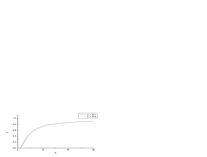
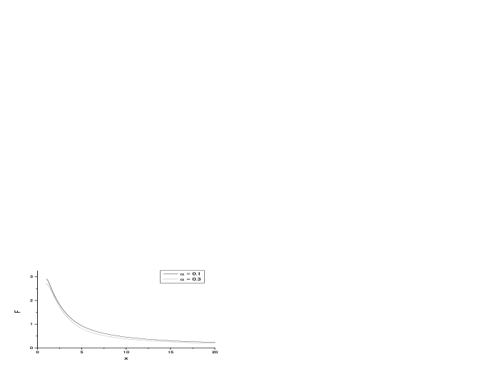
Figure 1: The metric function $f$ as a function of $x$ with $\theta=\pi/4$ and $x_{h}=1.0$.

Figure 2: The Skyrme function $F$ as a function of $x$ with $\theta=\pi/4$ and $x_{h}=1.0$.

Figure 3: The domain of existence of the solution. For $\alpha>0.37$, there exists no non-trivial solution.

Figure 4: A contour plot of the energy density $\epsilon$ in cylindrical coordinates $\rho$ and $z$ with $x_{h}=0.8$.

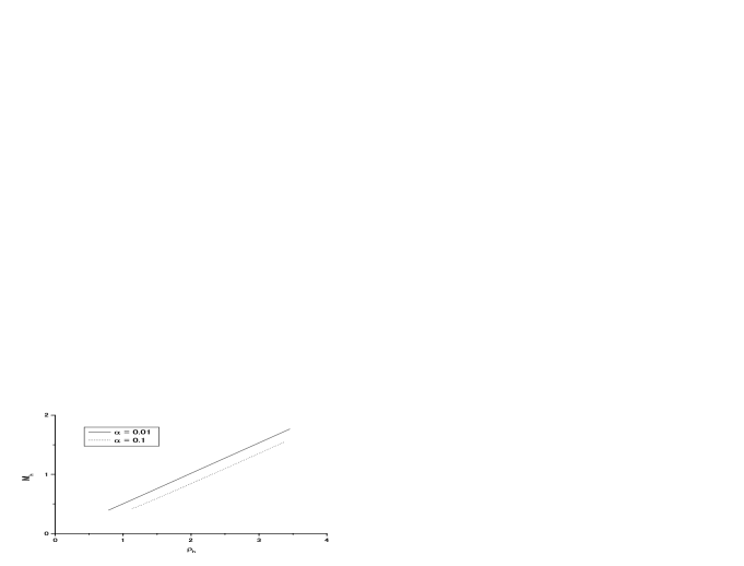
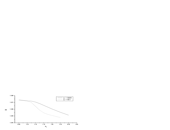
Figure 5: The horizon mass $M_{h}$ as a function of $\rho_{h}$.

Figure 6: The dependence of the baryon number on the size of the horizon.

References

• (1) R. Ruffini and J. A. Wheeler, Physics Today 24 (1971) 30.
• (2) H. Luckock and I. G. Moss, Phys. Lett. B176 (1986) 341; H. Luckock, String theory, quantum cosmology etc. Eds. H. J. de Vega and N. Sanchez (world scientific, 1987).
• (3) S. Droz, M. Heusler and N. Straumann, Phys. Lett. B268 (1991) 371.
• (4) M. S. Volkov and D. V. Galtsov, JETP Lett. 50 (1989) 346.
• (5) T.Torii and K. Maeda, Phys. Rev. D 48 (1993) 1643;
• (6) G. V. Lavrelashvili and D. Maison, Nucl. Phys. B410 (1993) 407.
• (7) K-M. Lee, V. P. Nair and E. J. Weinberg, Phys. Rev. D45 (1992) 2751.
• (8) B. Kleihaus and J. Kunz, Phys. Rev. Lett. 79 (1997) 1595.
• (9) B. Hartmann, B. Kleihaus and J. Kunz, Phys. Rev. D65 (2002) 024027.
• (10) E. Braaten and L. Carson, Phys. Rev. D38 (1988) 3525.
• (11) N. Arkani-Hamed, S. Dimopoulos and G. Dvali, Phys. Lett. B429 (1988) 263
• (12) M. Cavaglia, Int. J. Mod. Phys. A18 (2003) 1843
• (13) T. Banks and W. Fischler, hep-th/9906038
• (14) T. H. R. Skyrme, Proc. Roy. Soc. Lond. A260 (1961) 127.
• (15) A. Ashtekar, A. Corichi and D. Sudarsky, Class. Quant. Grav. 18 (2001) 919.
• (16) S. A. Ridgway and E. J. Weinberg, Phys. Rev. D52 (1995) 3440.
• (17) K. Maeda, T. Tachizawa, T. Torii and T. Maki, Phys. Rev. Lett. 72 (1994) 450; T. Torii, K. Maeda and T. Tachizawa, Phys. Rev. D51 (1995) 1510.
• (18) I. G. Moss, N. Shiiki and E. Winstanley, Class. Quant. Grav. 17 (2000) 4161