Radiation from accelerated black holes in an anti–de Sitter universe

Abstract

We study gravitational and electromagnetic radiation generated by uniformly accelerated charged black holes in anti–de Sitter spacetime. This is described by the $C$-metric exact solution of the Einstein-Maxwell equations with a negative cosmological constant $\Lambda$. We explicitly find and interpret the pattern of radiation that characterizes the dependence of the fields on a null direction from which the (timelike) conformal infinity is approached. This directional pattern exhibits specific properties which are more complicated if compared with recent analogous results obtained for asymptotic behavior of fields near a de Sitter-like infinity. In particular, for large acceleration the anti–de Sitter-like infinity is divided by Killing horizons into several distinct domains with a different structure of principal null directions, in which the patterns of radiation differ.

I Introduction

In the context of exact solutions of Einstein’s field equations, gravitational radiation has been studied for decades. In particular, various techniques have been developed to rigorously characterize asymptotic properties of the gravitational field, i.e., the geometry of spacetime at “large distance” from bounded sources.

In the fundamental work Bondi et al. (1962) gravitational waves emitted by axisymmetric systems were analyzed by considering an expansion of metric functions in inverse powers of an appropriate “radial” coordinate $r$ parametrizing outgoing null geodesics. In particular, the news function was defined that characterizes radiation, and which is related to a decreasing (Bondi) mass of the source. Generalizations and refinement of this method, with a deeper understanding of its relation to the Petrov types (such as the peeling-off behavior of the Weyl tensor) were subsequently achieved in Sachs (1962); Newman and Penrose (1962); Newman and Unti (1962); van der Burg (1969); Bičák and Pravdová (1998), see, e.g., Pirani (1965); Bičák (1985, 1997, 2000) for reviews. Nevertheless, in these works the analysis of radiative fields remained confined to asymptotically flat spacetimes thus ruling out, for instance, the presence of a nonvanishing cosmological constant $\Lambda$. In addition, it was based on the use of privileged coordinate systems.

It was Penrose Penrose (1963, 1964, 1965), see Penrose and Rindler (1986) for a comprehensive overview, who introduced a covariant approach to the definition of radiation for massless fields, which is based on the conformal treatment of infinity (a comparison of the Bondi-Sachs and Penrose approaches was recently presented in Tafel and Pukas (2000)). This enables one to apply methods of local differential geometry “at infinity”, and thus to define in a rigorous geometric way such basic concepts as the Bondi mass, the peeling-off property, and the Bondi-Metzner-Sachs group of asymptotic symmetries. In particular, gravitational radiation propagating along a given null geodesic is described by the $\Psi_{4}$ component of the Weyl tensor projected on a parallelly transported complex null tetrad at infinity. The crucial point is that such a tetrad is (essentially) determined uniquely by the conformal geometry Penrose and Rindler (1986). Moreover, an advantage of the Penrose method is that it can be naturally applied also to asymptotically simple spacetimes which include the cosmological constant Penrose (1964, 1965); Penrose and Rindler (1986). This is quite remarkable since there is no analogue of the news function in the presence of $\Lambda$ Ashtekar and Magnon (1984); Ashtekar and Das (2000).

However, specific new features appear in the case of asymptotically de Sitter ($\Lambda>0$) or anti–de Sitter ($\Lambda<0$) spacetimes, for which the conformal infinity ${\mathcal{I}}$ is, respectively, spacelike or timelike Penrose (1964, 1965); Penrose and Rindler (1986); Penrose (1967). First of all, the concept of radiation for a massless field is “less invariant” in cases when ${\mathcal{I}}$ is not null. Namely, it emerges as necessarily direction dependent since the choice of the above-mentioned null tetrad, and thus the radiative component $\Psi_{4}$ of the field, turns out to be different for different null geodesics reaching the same point on ${\mathcal{I}}$. This is related to the fact that with nonvanishing $\Lambda$ even fields of nonaccelerated sources are radiative along a generic direction, as it has been shown for test charges Bičák and Krtouš (2002) or for Reissner-Nordström black holes Krtouš and Podolský (2003) in a de Sitter universe, and it will be shown here for a negative $\Lambda$ (Sec. V.3). In addition, the character of infinity plays a crucial role in the formulation of the initial value problem. A spacelike ${\mathcal{I}}$ implies the insufficiency of purely retarded massless fields so that, for example, in de Sitter space purely retarded solutions of the Maxwell equations are impossible for generic charge distributions Bičák and Krtouš (2001). On the other hand, it is wellknown that a timelike ${\mathcal{I}}$ prevents the existence of a Cauchy surface, and one is necessarily led to a kind of “mixed initial value boundary problem”, see, e.g., Avis et al. (1978); Hawking (1983); Friedrich (1995). For all the above reasons, the definition of radiation is much less obvious when ${\Lambda\not=0}$.

Any explicit exact example of a source which generates gravitational waves in an (anti–)de Sitter universe is thus of paramount importance since this may provide us with insight into the character of radiation in spacetimes which are not asymptotically flat. Exact solutions with boost-rotation symmetry Bičák and Schmidt (1989); Bičák (1968); Pravda and Pravdová (2000), which represent radiative spacetimes with uniformly accelerating sources, play a unique role when ${\Lambda=0}$. Among these the $C$-metric, which describes accelerated black holes, admits a natural generalization to a nonvanishing value of the cosmological constant, and it will thus be considered in the present paper.

The $C$-metric Levi-Civita (1917); Weyl (1918); Ehlers and Kundt (1962); Kramer et al. (1980) is a classic solution of the Einstein(-Maxwell) equations which has been physically interpreted and analyzed in fundamental papers Kinnersley and Walker (1970); Farhoosh and Zimmerman (1979); Ashtekar and Dray (1981); Bonnor (1983) and in many other works, see e.g. Bičák and Schmidt (1989); Bičák and Pravda (1999); Pravda and Pravdová (2000); Letelier and Oliveira (2001); Dias and Lemos (2003a) for references and summary of the results. A generalization of the standard $C$-metric to admit a nonvanishing value of $\Lambda$ has also been known for a long time Plebański and Demiański (1976), cf. Carter (1968); Debever (1971) (also, related solutions have been obtained by considering extremal limits of the $C$-metric with an arbitrary $\Lambda$ Dias and Lemos ). These spacetimes have found successful application to the problem of cosmological pair creation of black holes Mann and Ross (1995); Mann (1997, 1998); Booth and Mann (1999). However, a deeper understanding of their physical and global properties, including the character of radiation, has been missing until recently. The interpretation of the $C$-metric solutions with ${\Lambda>0}$, in particular the meaning of parameters in the metric and the relation to the “background” de Sitter universe, was clarified in Podolský and Griffiths (2001) by introducing an appropriate coordinate system adapted to uniformly accelerated observers. The causal structure was further studied in Dias and Lemos (2003b) for various choices of the physical parameters. Very recently Krtouš and Podolský (2003), we have carefully analyzed the $C$-metric with ${\Lambda>0}$ and, among other results, we have demonstrated that gravitational and electromagnetic fields of this exact solution exhibit asymptotically a specific directional pattern of radiation at ${\mathcal{I}}$. Interestingly, this directional dependence of fields on null directions from which the conformal infinity is approached is the same as for the test fields of uniformly accelerated charges in a de Sitter universe Bičák and Krtouš (2002).

In the present work we wish to investigate an analogous asymptotic behavior of fields of the $C$-metric with ${\Lambda<0}$, i.e., the directional dependence at conformal infinity ${\mathcal{I}}$ of radiation generated by uniformly accelerated (possibly charged) black holes in an anti–de Sitter universe. Some fundamental differences from the cases ${\Lambda\geq 0}$ appear since ${\mathcal{I}}$ now has a timelike character. In fact, the whole structure of the “anti–de Sitter $C$-metric” is much more complex and new peculiar phenomena thus occur. As observed in Emparan et al. (2000b) and thoroughly studied in the recent work Dias and Lemos (2003a), for a small value of acceleration, ${A<\sqrt{-\Lambda/3}}$, the metric describes a single uniformly accelerated black hole in an anti–de Sitter universe Podolský (2002) whereas for ${A>\sqrt{-\Lambda/3}}$ this represents a pair of accelerated black holes. The “limiting case” given by ${A=\sqrt{-\Lambda/3}}$, previously investigated in Emparan et al. (2000a); Chamblin (2001), plays a special important role in the context of the Randall-Sundrum model since it describes a black hole bound to a two-brane in four dimensions. However, this case is not investigated in the present work.

Our paper is organized as follows. First, in Sec. II we present the $C$-metric solution with a negative cosmological constant, in particular the Robinson-Trautman coordinates which will be used in the subsequent analysis. Basic properties of the solution are also summarized, including a description of the global structure. Secs. III–V contain the core of our analysis. First we define a suitable interpretation tetrad parallelly transported along null geodesics approaching asymptotically a given point on conformal infinity ${\mathcal{I}}$ from all possible spacetime directions. The magnitude of the leading terms of gravitational and electromagnetic fields in such a tetrad then provides us with a specific directional pattern of radiation. Convenient parametrizations of null directions approaching ${\mathcal{I}}$ are introduced in Sec. IV, and the results are subsequently described and analyzed in Sec. V. This is done for both the cases of a single black hole and a pair of black holes accelerating in an anti–de Sitter universe (and for vanishing acceleration). The paper also contains two appendixes. In Appendix A the behavior of radiation along special null directions is studied. In particular, for geodesics along principal null directions the results are obtained in closed explicit form without performing asymptotic expansions of the physical quantities near ${{\mathcal{I}}}$. Appendix B summarizes the Lorentz transformations of the null-tetrad components of the gravitational and electromagnetic fields.

II The $C$-metric with a negative cosmological constant

The $C$-metric with a cosmological constant ${\Lambda<0}$, contained in the family of solutions Plebański and Demiański (1976), can be written as

$${\boldsymbol{g}}=\frac{1}{A^{2}(x+y)^{2}}\Bigl{(}-F\,\mathbf{d}t^{2}+\frac{1}{F}\,\mathbf{d}y^{2}+\frac{1}{G}\,\mathbf{d}x^{2}+G\,\mathbf{d}\varphi^{2}\Bigr{)}{\mbox{\;,}}$$ (1)

where $F$ and $G$ are, respectively, polynomials of $y$ and $x$,

$$F =\frac{-\Lambda}{\ \>3A^{2}}-1+y^{2}-2mA\,y^{3}+e^{2}A^{2}\,y^{4}{\mbox{\;,}}$$ (2)

$$G =\mspace{67.0mu}1-x^{2}-2mA\,x^{3}-e^{2}A^{2}\,x^{4}{\mbox{\;.}}$$

These functions are mutually related by

$$F=-{\mathrm{Q}}(y)+\frac{-\Lambda}{\ \>3A^{2}}{\mbox{\;,\quad}}G={\mathrm{Q}}(-x){\mbox{\;,}}$$ (3)

where ${{\mathrm{Q}}(w)}=1-w^{2}+2\,mA\,w^{3}-e^{2}A^{2}\,w^{4}$. The metric (1) is a solution of the Einstein-Maxwell equations with a non-null electromagnetic field given by

$${\boldsymbol{\mathbf{F}}}=e\,\mathbf{d}y\wedge\mathbf{d}t{\mbox{\;,}}$$ (4)

or related expressions which can be obtained by a constant duality rotation. There exist two double-degenerate principal null directions (PNDs)

$${{\boldsymbol{\mathbf{k}}}}_{1}\propto{{\boldsymbol{\mathbf{\partial}}}_{t}}-F{{\boldsymbol{\mathbf{\partial}}}_{y}}{\mbox{\;,\quad}}{{\boldsymbol{\mathbf{k}}}}_{2}\propto{{\boldsymbol{\mathbf{\partial}}}_{t}}+F{{\boldsymbol{\mathbf{\partial}}}_{y}}{\mbox{\;,}}$$ (5)

so that the spacetime is of the Petrov type $D$. It admits two Killing vectors ${{\boldsymbol{\mathbf{\partial}}}_{t}}$, ${{\boldsymbol{\mathbf{\partial}}}_{\varphi}}$, and one conformal Killing tensor ${\boldsymbol{\mathbf{Q}}}$ (cf. Refs. Walker and Penrose (1970); Hughston et al. (1972); Penrose and Rindler (1986)),

$${\boldsymbol{\mathbf{Q}}}=\frac{1}{A^{4}(x+y)^{4}}\Bigl{(}F\,\mathbf{d}t^{2}-\frac{1}{F}\,\mathbf{d}y^{2}+\frac{1}{G}\,\mathbf{d}x^{2}+G\,\mathbf{d}\varphi^{2}\Bigr{)}{\mbox{\;.}}$$ (6)

The metric (1) can describe different spacetimes, depending on the choice of parameters and of ranges of coordinates. We are interested in the physically most relevant case when the metric describes one black hole or pairs of black holes uniformly accelerated in anti–de Sitter universe. In this case the constants $A$, $m$, $e$, and $C$, such that ${\varphi\in(-\pi C,\pi C)}$, characterize acceleration, mass, charge of the black holes, and conicity of the $\varphi$ symmetry axis, respectively. They have to satisfy $m\geq 0$, $e^{2}<m^{2}$, ${A,\,C>0}$, and they have to be such that the function $G$ has four real roots in the charged case (${e,\,m\neq 0}$) or three real roots in the uncharged case (${e=0}$, ${m\neq 0}$). The coordinates ${x,\,y}$ have to satisfy ${y>-x}$ and ${x\in[x_{\mathrm{f}},x_{\mathrm{b}}]}$, where ${x_{\mathrm{f}}<0<x_{\mathrm{b}}}$ are two roots of $G$, namely those closest to zero (see Krtouš and Podolský (2003); Mann (1997); Podolský (2002); Dias and Lemos (2003a) for details and discussion of other cases, cf. also Figs. 1(d) and 3 below). From these conditions we obtain $0\leq G\leq 1$, and $m+2e^{2}A\,x>0$. The spacetime (1) reduces to the anti–de Sitter universe for ${m=0,\,e=0}$.

The coordinates $x$ and $\varphi$ are longitudinal and latitudinal angular coordinates, $x_{\mathrm{f}}$ denotes the axis of $\varphi$ symmetry extending from the “forward” pole of the black hole (in the direction of acceleration) to infinity, whereas $x_{\mathrm{b}}$ denotes the axis from the opposite “backward” pole. For nonvanishing acceleration the axis cannot be regular everywhere — at least one part of it has to have a nontrivial conicity, depending on the choice of the parameter $C$. This corresponds to the presence of cosmic strings (or struts) which are responsible for the acceleration of the black holes, see the references above for more details.

The spacetime metric (1) can be put into various forms. In this paper we concentrate on investigation of radiation near infinity, for which the Robinson-Trautman form seems to be a convenient one. Introducing real coordinates $r$, $u$ and complex coordinates ${\zeta,\,\bar{\zeta}}$ by

$$A\,r =(x+y)^{-1}{\mbox{\;,}}$$ (7)

$$A\,\mathbf{d}u =\frac{\mathbf{d}y}{F}+\mathbf{d}t{\mbox{\;,}}$$

$$\textstyle{\frac{1}{\sqrt{2}}}(\mathbf{d}\zeta+\mathbf{d}\bar{\zeta}) =\frac{\mathbf{d}y}{F}-\frac{\mathbf{d}x}{G}+\mathbf{d}t{\mbox{\;,}}$$

$$\textstyle{\frac{i}{\sqrt{2}}}(\mathbf{d}\zeta-\mathbf{d}\bar{\zeta}) =\mathbf{d}\varphi{\mbox{\;,}}$$

we put the $C$-metric (1) into the form

$${\boldsymbol{g}}=\frac{r^{2}}{P^{2}}\,\mathbf{d}\zeta\mathbin{\scriptstyle{\vee}}\mathbf{d}\bar{\zeta}-\mathbf{d}u\mathbin{\scriptstyle{\vee}}\mathbf{d}r-H\,\mathbf{d}u^{2}{\mbox{\;.}}$$ (8)

The metric functions are

$$P^{-2}=G{\mbox{\;,}}\qquad\ H=A^{2}r^{2}(F+G){\mbox{\;,}}$$ (9)

or explicitly

$$H =-\frac{\Lambda}{3}\,r^{2}-2\,r\,(\ln P)_{,u}+\Delta\ln P$$ (10)

$$\qquad\qquad\quad-\frac{2}{r}(m+2e^{2}A\,x)+\frac{e^{2}}{r^{2}}{\mbox{\;,}}$$

with ${\Delta=2P^{2}\partial_{\zeta}\partial_{\bar{\zeta}}}$, where $x$ is expressed using the relation

$$\int\frac{dx}{G(x)}=A\,u-\textstyle{\frac{1}{\sqrt{2}}}(\zeta+\bar{\zeta}){\mbox{\;.}}$$ (11)

The functions (9), (10) represent a particular case, corresponding to the $C$-metric, of the standard general expression for the Robinson-Trautman spacetimes Kramer et al. (1980). As opposed to the metric form (1), the Robinson-Trautman coordinates allow an explicit limit ${A=0}$. The coordinates are not defined globally but it is possible to cover the whole universe by many coordinate patches of the same type. Therefore, it is sufficient to study the spacetime only in just one Robinson-Trautman coordinate map; such a patch is indicated by a shaded domain in Figs. 4–6. We additionally assume there that the coordinate $u$ is increasing from the past to the future.

The global causal structure of the $C$-metric with ${\Lambda<0}$ has recently been analyzed in Dias and Lemos (2003a). In particular, the character of infinity, singularities, and possible horizons has been described in detail.

Infinity ${\mathcal{I}}$ of the spacetime is given by

$$r=\infty{\mbox{\;,\quad}}\text{or equivalently}\quad x+y=0{\mbox{\;,}}$$ (12)

where the conformal factor

$$\Omega=\frac{1}{r}=A(x+y)$$ (13)

vanishes. The conformal (unphysical) metric ${\bf\tilde{{\boldsymbol{g}}}}=\Omega^{2}{\boldsymbol{g}}{\mbox{\;,}}$

$$\tilde{{\boldsymbol{g}}}=\frac{1}{P^{2}}\,\mathbf{d}\zeta\mathbin{\scriptstyle{\vee}}\mathbf{d}\bar{\zeta}+\mathbf{d}u\mathbin{\scriptstyle{\vee}}\mathbf{d}\Omega-H\,\Omega^{2}\mathbf{d}u^{2}{\mbox{\;.}}$$ (14)

is regular at infinity, given by $\Omega=0$. Moreover, it follows from Eq. (10) that at ${\mathcal{I}}$ the metric function reads

$$H\,\Omega^{2}\Big{|}_{{\mathcal{I}}}=-\frac{\Lambda}{3}{\mbox{\;,}}$$ (15)

i.e.. it is independent of the parameters $m$, $e$, and $A$. The vector ${{{{\boldsymbol{\mathbf{n}}}}_{\scriptscriptstyle\mathrm{P}}}=-(H\Omega^{2}{{\boldsymbol{\mathbf{\partial}}}_{\Omega}}+{{\boldsymbol{\mathbf{\partial}}}_{u}})}$ is orthogonal to each hypersurface $\Omega=\rm{constant}$. In particular, it is outgoing and normal to infinity ${\mathcal{I}}$ at any of its point, with the norm ${{\bf\tilde{{\boldsymbol{g}}}}({{{\boldsymbol{\mathbf{n}}}}_{\scriptscriptstyle\mathrm{P}}},{{{\boldsymbol{\mathbf{n}}}}_{\scriptscriptstyle\mathrm{P}}})=H\Omega^{2}=-\frac{\Lambda}{3}>0}$. The universe is thus weakly asymptotically anti–de Sitter Ashtekar and Magnon (1984), at least locally, with the conformal infinity ${\mathcal{I}}$ having a timelike character (in general, it is not asymptotically anti–de Sitter according to the definition based on the “reflective boundary condition” Hawking (1983); Ashtekar and Magnon (1984); Henneaux and Teitelboim (1985); Ashtekar and Das (2000): the ${(2+1)}$-metric induced on ${\mathcal{I}}$ by ${\bf\tilde{{\boldsymbol{g}}}}$ is not conformally flat since the associated Bach tensor is nonvanishing). Throughout the paper, however, it will be more convenient to employ the spacelike outward vector ${{{\boldsymbol{\mathbf{n}}}}={{{\boldsymbol{\mathbf{n}}}}_{\scriptscriptstyle\mathrm{P}}}/\sqrt{H}}$ orthogonal to ${\mathcal{I}}$,

$${{\boldsymbol{\mathbf{n}}}}=\sqrt{H}\,{{\boldsymbol{\mathbf{\partial}}}_{r}}-\frac{1}{\sqrt{H}}\,{{\boldsymbol{\mathbf{\partial}}}_{u}}{\mbox{\;,}}$$ (16)

which has a unit norm ${{{\boldsymbol{\mathbf{n}}}}\mathbin{\boldsymbol{\cdot}}{{\boldsymbol{\mathbf{n}}}}={\boldsymbol{g}}({{\boldsymbol{\mathbf{n}}}},{{\boldsymbol{\mathbf{n}}}})=1}$ with respect to the physical metric.

At ${r=0}$ the metric has unbounded curvature which corresponds to a physical singularity hidden behind the black hole horizon. Similarly to the $C$-metric with vanishing $\Lambda$ Kinnersley and Walker (1970); Farhoosh and Zimmerman (1979); Ashtekar and Dray (1981); Bonnor (1983); Bičák and Pravda (1999); Letelier and Oliveira (2001) or the $C$-metric with ${\Lambda>0}$ Podolský and Griffiths (2001); Dias and Lemos (2003b); Krtouš and Podolský (2003), the zeros of the function $F$ correspond to Killing horizons associated with ${{\boldsymbol{\mathbf{\partial}}}_{t}}$. Interestingly, unlike in the ${\Lambda\geq 0}$ case, the anti–de Sitter $C$-metric describes either a single uniformly accelerated black hole (for ${A<\sqrt{-\Lambda/3}}$ ), or a pair of uniformly accelerated black holes (when ${A>\sqrt{-\Lambda/3}}$ ).

II.1 A single accelerated black hole

Indeed, as described in Podolský (2002); Dias and Lemos (2003a), when the acceleration parameter $A$ is small, namely ${A<\sqrt{-\Lambda/3}}$, and $m\neq 0$, the metric (1), (2) describes a single uniformly accelerated black hole. The condition of small acceleration guarantees that the function $F$ has only two zeros ${y_{\mathrm{o}}},\,{y_{\mathrm{i}}}$ in the charged case, or only one zero ${y_{\mathrm{o}}}$ for the uncharged black hole. These zeros define outer and, if applicable, inner horizons of the black hole. The relevant ranges of coordinates $x,\,y$ representing the spacetime outside the black hole are depicted in Fig. 1(d).

In Dias and Lemos (2003a) the causal structure of this spacetime was represented by the Penrose-Carter conformal diagram of a two-dimensional ${t{\text{-}}y}$ section (i.e., the section of constant angular coordinates ${x,\,\varphi}$). This section is, in fact, spanned by the PNDs ${{\boldsymbol{\mathbf{k}}}}_{1}$ and ${{\boldsymbol{\mathbf{k}}}}_{2}$, cf. Eq. (5). A part of such a conformal diagram representing an exterior of the black hole is depicted in Fig. 1(c). The conformal infinity ${\mathcal{I}}$ is indicated here by a double line. The outer horizons ${\mathcal{H}}_{\mathrm{o}}$, given by ${y={y_{\mathrm{o}}}}$, separate region II outside the black hole from an interior of the black hole, denoted as III. A more detailed structure of the interior of the black hole depends on whether the hole is charged or not, and its causal structure is analogous to the Schwarzschild or Reissner-Nordström black holes. Because we are mainly interested in region II near the infinity, we will not discuss the interior of the hole here.

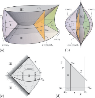
Figure 1: Spacetime outside a single accelerated black hole moving in an anti–de Sitter universe with acceleration ${A<\sqrt{-\Lambda/3}}$. Diagrams (a) and (b) depict a three-dimensional section ${\varphi=\text{constant}}$, diagram (c) is a conformal diagram of the ${t{\text{-}}y}$ section, and diagram (d) shows relevant ranges of coordinates $x$ and $y$. The diagrams focus on region II between the outer black hole horizon ${\mathcal{H}}_{\mathrm{o}}$ (${y={y_{\mathrm{o}}}}$) and timelike infinity ${\mathcal{I}}$, ${y=-x}$. Therefore, only a small part of an interior of the black hole near the horizon ${\mathcal{H}}_{\mathrm{o}}$ is shown (region III). In diagram (a) the horizon ${\mathcal{H}}_{\mathrm{o}}$ is represented by two conical surfaces which intersect on a bifurcation surface of the Killing vector ${{\boldsymbol{\mathbf{\partial}}}_{t}}$ (a continuation of cones inside the black hole to another asymptotic domain is not shown). The outer deformed boundary of domain II corresponds to infinity ${\mathcal{I}}$. A particular section ${\mathcal{S}}$ given by ${x=\text{constant}}$ is shown, and the axes ${x=x_{\mathrm{b}}}$ and ${x=x_{\mathrm{f}}}$ are indicated. It is assumed in diagram (a) that the string causing acceleration of the black hole is located on the “forward” axis ${x=x_{\mathrm{f}}}$ and the corresponding conical singularity is represented by nonsmooth behavior at ${\mathcal{S}_{S}}$ (the edge at ${x=x_{\mathrm{f}}}$). Diagram (b) is a deformation of diagram (a) in which both the top and the bottom of the diagram are squeezed to single points, and the longitudinal $x$ direction is embedded smoothly at both axes. The black hole horizon ${\mathcal{H}}_{\mathrm{o}}$ has thus a droplike shape, symmetrical around the vertical axis. Diagram (c) is the Penrose-Carter conformal diagram of the ${t{\text{-}}y}$ section ${\mathcal{S}}$ (${x,\varphi=\text{constant}}$). Both principal null directions lie in this section. The precise shape of infinity ${\mathcal{I}}$ (double line) depends on the value of coordinate $x$, cf. Eq. (12) [and this dependence is the reason for the deformed shape of ${\mathcal{I}}$ in diagram (a)]. Lines ${t=\text{constant}}$, and ${y=\text{constant}}$ (coinciding with ${r=\text{constant}}$ in ${\mathcal{S}}$) are drawn with labels oriented in the direction of an increasing coordinate. A small part of the interior of the black hole is indicated by the dark area at the left of the diagram. Finally, diagram (d) depicts the ${x{\text{-}}y}$ section for relevant ranges of coordinates (shaded area). The infinity is again represented by the double line, and the horizon ${\mathcal{H}}_{\mathrm{o}}$ is shown. The thick line ${x=\text{constant}}$ corresponds to the ${t{\text{-}}y}$ section of diagram (c), similarly the thick line ${t=\text{constant}}$ in diagram (c) corresponds to the ${x{\text{-}}y}$ section from diagram (d).

It seems to be more instructive to combine the ${t{\text{-}}y}$ sections for different values of $x$ into a unifying three-dimensional picture in which just the coordinate $\varphi$ is suppressed, as it is done in Fig. 1(a). Despite the fact that this is not a complete and rigorous conformal diagram, it helps to visualize and understand the global causal structure of the spacetime. The outer horizon ${\mathcal{H}}_{\mathrm{o}}$ of the black hole is here indicated by two joined conical surfaces, and the conformal timelike infinity ${\mathcal{I}}$ is depicted as a deformed outer boundary. It has a “simple” topology ${{\mathbb{R}}\times\mathrm{S}^{2}}$ if we include “nonsmooth” points on the $\varphi$ axis where the string is located. For a vanishing acceleration the timelike infinity would be rotationally symmetric around the vertical axis, and smooth everywhere. Its deformation for ${A\neq 0}$ indicates that the coordinates are adapted to the accelerated source (for an analogous discussion in the ${\Lambda>0}$ case see Krtouš and Podolský (2003)) and that there is a string (a conical singularity) on the $\varphi$ axis. Particular surfaces ${\mathcal{S}}$ of a constant $x$, corresponding to the two-dimensional conformal diagram 1(c), are also indicated. The section ${\mathcal{S}_{S}}$ with ${x=x_{\mathrm{f}}}$ corresponds to the axis from the “forward” pole of the black hole, the value ${x=x_{\mathrm{b}}}$ to the axis from the opposite “backward” pole. In Fig. 1(a) the conicity parameter $C$ is chosen in such a way that the string is located only on the axis ${x=x_{\mathrm{f}}}$, and the conical singularity is indicated by nonsmooth embedding of the ${t,\,y=\text{constant}}$ surface into the three-dimensional diagram, i.e., by a nonsmooth gluing of ${x=\text{constant}}$ sections at $x_{\mathrm{f}}$. Notice that since ${F>0}$ for $y<{y_{\mathrm{o}}}$, region II near infinity ${\mathcal{I}}$ is everywhere static, and there are no Killing horizons which extend up to ${\mathcal{I}}$ [cf. also Eqs. (67), (68)]. We can thus interpret the spacetime as a universe having global anti–de Sitter-like infinity (except the nonsmoothness at the string) with the black hole moving “inside” it (in contrast to the case discussed below, where pairs of black holes “enter” and “exit” the spacetime “through” the infinity).

The diagram 1(b) is a deformed version of the diagram 1(a): gluing of the angular coordinate $x$ is now done smoothly even on the axis where the string is located, and the top and the bottom of the diagram are “squeezed” to single points. The horizon ${\mathcal{H}}_{\mathrm{o}}$ thus has a shape of two joined “drops”, and sections ${x=\text{constant}}$ are deformed accordingly. Here we can see that coordinates $t,\,y,\,x,\,\varphi$ used to construct this diagram are adapted to the source, not to the infinity — the horizon ${\mathcal{H}}_{\mathrm{o}}$ is symmetric around the vertical axis in contrast to infinity ${\mathcal{I}}$ which is deformed in the direction of acceleration. Diagram 1(b) is not so crucial in the present case of a single black hole but an analogous representation of the black hole horizon will be used in the case of two accelerated holes which we are going to discuss now.

II.2 A pair of accelerated black holes

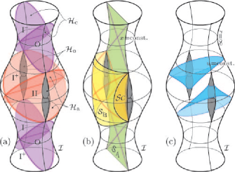
Figure 2: Schematic diagrams of a part of spacetime outside accelerated black holes moving in an anti–de Sitter universe with acceleration ${A>\sqrt{-\Lambda/3}}$. Diagrams represent a three-dimensional section ${\varphi=\text{constant}}$. They depict a domain near one pair of black holes. However, they should continue periodically in a vertical direction, featuring thus an infinite chain of pairs of black holes entering and later exiting the spacetime through timelike infinity ${\mathcal{I}}$. Only regions of spacetime outside the outer black hole horizons ${\mathcal{H}}_{\mathrm{o}}$ are drawn. Interiors of black holes and continuations of the spacetime into other asymptotically anti–de Sitter universes (through the Einstein-Rosen bridge or through charged black hole) are hidden under the horizons ${\mathcal{H}}_{\mathrm{o}}$ and not studied in the paper. The outer black hole horizons ${\mathcal{H}}_{\mathrm{o}}$ are represented by droplike gray shapes analogous to that of Fig. 1(b), the timelike infinity ${\mathcal{I}}$ is depicted as a deformed cylindrical boundary of the diagrams. Diagram (a) shows the Killing horizons outside the black holes: acceleration horizons ${\mathcal{H}}_{\mathrm{a}}$ separating two black holes, and cosmological horizons ${\mathcal{H}}_{\mathrm{c}}$ separating different pairs of black holes (only one pair of holes is drawn in the diagram). These horizons divide spacetime into several regions: static domains O and II, nonstatic domains ${\mathrm{I}^{+}}$ and ${\mathrm{I}^{-}}$, and domains inside the holes hidden under ${\mathcal{H}}_{\mathrm{o}}$. Diagram (b) indicates embedding of ${t{\text{-}}y}$ sections for different constant values of the coordinate $x$, which are spanned by principal null directions. Three qualitatively different sections ${\mathcal{S}_{A}}$, ${\mathcal{S}_{B}}$, and ${\mathcal{S}_{C}}$ are shown. Exact conformal diagrams corresponding to these sections can be found in Figs. 4–6. Diagram (c) shows hypersurfaces ${u=\text{constant}}$ which are generated by null geodesics along the principal null directions ${{\boldsymbol{\mathbf{k}}}}_{1}$ that are discussed in Appendix A.

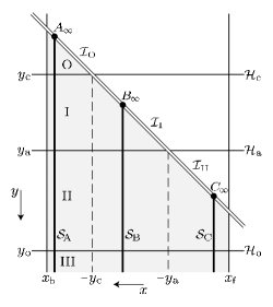
Figure 3: A qualitative ${x{\text{-}}y}$ diagram in the case of large acceleration ${A>\sqrt{-\Lambda/3}}$ (cf. Fig. 1(d) for small acceleration). The relevant domain of coordinates $x$ and $y$ is indicated by the shaded area. It is given by the coordinate $x$ between the axes $x_{\mathrm{f}}$ and $x_{\mathrm{b}}$, and the coordinate $y$ between the infinity ${\mathcal{I}}$, ${y=-x}$, and the outer black hole horizon ${\mathcal{H}}_{\mathrm{o}}$, ${y={y_{\mathrm{o}}}}$ (the interior of black holes, ${y>{y_{\mathrm{o}}}}$, is not studied here). The infinity is represented by a double line, the horizons by horizontal lines. The ${t{\text{-}}y}$ sections of constant $x$ are represented by vertical lines. Three such typical sections ${\mathcal{S}_{A}}$, ${\mathcal{S}_{B}}$ and ${\mathcal{S}_{C}}$ are shown. They are distinguished by the number of horizons which they intersect. These sections correspond to the conformal diagrams in Figs. 4–6. ${A_{\scriptscriptstyle{\infty}},B_{\scriptscriptstyle{\infty}},C_{\scriptscriptstyle{\infty}}}$ are points at the infinity which belong to these three sections, respectively. They can be found also in Figs. 4–6.

A more complicated situation occurs when ${A>\sqrt{-\Lambda/3}}$, ${m\neq 0}$. For such large values of acceleration the metric (1), (2) describes an infinite number of pairs of accelerated black holes in anti–de Sitter universe. In Fig. 2, representing a part of the section ${\varphi=\text{constant}}$, one pair of black holes is indicated by the (outer) horizons ${\mathcal{H}}_{\mathrm{o}}$ which have droplike shapes analogous to the horizon in diagram 1(b). The main difference from the previous case is that both black holes “simultaneously enter” the universe at infinity ${\mathcal{I}}$, approach each other with an opposite deceleration until they stop, and start to move apart, again up to the infinity ${\mathcal{I}}$. The same situation repeats infinitely many times both in the past and in the future — the diagrams in Fig. 2 should be infinitely long, composed of parts isomorphic to the part shown there. In the following we study only one such part of the whole universe. Relevant ranges of coordinates $x$ and $y$ are drawn in Fig. 3.

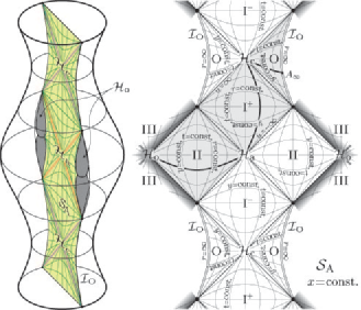
Figure 4: Conformal diagram of the ${t{\text{-}}y}$ section ${\mathcal{S}_{A}}$ intersecting both the horizons ${\mathcal{H}}_{\mathrm{a}}$, ${\mathcal{H}}_{\mathrm{c}}$ outside black holes (right), and its embedding into three-dimensional diagram ${\varphi=\text{constant}}$ (left). Each of sections of constant $x$ (and $\varphi$) with ${x\in(-{y_{\mathrm{c}}},x_{\mathrm{b}}]}$ intersects all horizons and extends through the whole spacetime. Both three-dimensional and two-dimensional diagrams should continue periodically in the vertical direction. In the two-dimensional conformal diagram the infinity ${\mathcal{I}}$ is depicted by double lines. Section ${\mathcal{S}_{A}}$ intersects the infinity in a timelike surface belonging to domain ${\mathcal{I}}_{\,\mathrm{O}}$, cf. Fig. 10. Cosmological horizons ${\mathcal{H}}_{\mathrm{c}}$, acceleration horizons ${\mathcal{H}}_{\mathrm{a}}$, and outer black hole horizons ${\mathcal{H}}_{\mathrm{o}}$ are represented by diagonal lines. Domains between the horizons are labeled as O, ${\mathrm{I}^{\pm}}$, II, and III, cf. Fig. 2(a). Interiors of black holes are indicated only partially, by the dark area behind the horizon ${\mathcal{H}}_{\mathrm{o}}$. Lines of coordinates $t$ and $y$ are shown with labels oriented in direction of an increasing coordinate. An area covered by one Robinson-Trautman coordinate map (coordinates $u$, $r$) is indicated by the shaded background. Without the loss of a typical behavior, the special section ${x=x_{\mathrm{b}}}$ has been chosen for this diagram; other sections with ${x>-{y_{\mathrm{c}}}}$ look qualitatively the same, only with embedding not lying in the plane of symmetry of the three-dimensional diagram.

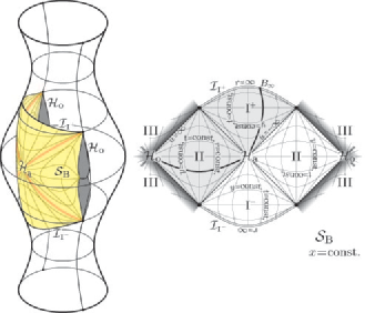
Figure 5: Conformal diagram of the ${t{\text{-}}y}$ section ${\mathcal{S}_{B}}$ intersecting only the horizons ${\mathcal{H}}_{\mathrm{a}}$ outside black holes, and its embedding into three-dimensional diagram ${\varphi=\text{constant}}$. Such a section of constant $x$ (and $\varphi$) with ${x\in(-{y_{\mathrm{a}}},-{y_{\mathrm{c}}})}$ intersects all horizons except the cosmological ones. In contrast to section ${\mathcal{S}_{A}}$ of Fig. 4, section ${\mathcal{S}_{B}}$ does not extend through the whole spacetime, but it can be found near all pairs of black holes. The section still extends between both holes of a given pair. Section ${\mathcal{S}_{B}}$ intersects the infinity in two spacelike surfaces, one forming a future boundary of ${\mathcal{S}_{B}}$ belonging to domain ${\mathcal{I}}_{\,{\mathrm{I}^{+}}}$, the other forming a past boundary belonging to domain ${\mathcal{I}}_{\,{\mathrm{I}^{-}}}$, cf. Fig. 10. Notation for infinity, horizons, etc., is the same as in Fig. 4. The shaded area again indicates Robinson-Trautman coordinate patch.

Clearly, both the global causal structure of the spacetime and the algebraic structure are now more complex. The metric function $F$ has two more zeros, ${y_{\mathrm{a}}}$ and ${y_{\mathrm{c}}}$, which correspond to the two additional Killing horizons outside of the black holes. We shall refer to these as acceleration horizons ${\mathcal{H}}_{\mathrm{a}}$, and cosmological horizons ${\mathcal{H}}_{\mathrm{c}}$. In contrast to the black hole horizons, spatial sections of these horizons are noncompact. The horizons are represented by inclined planes in Fig. 2(a) or as corresponding horizontal lines in Fig. 3. They separate static and nonstatic regions of the spacetime outside of the black holes: the domains O and II are static, whereas the domains ${\mathrm{I}^{+}}$ and ${\mathrm{I}^{-}}$ are nonstatic. Regions II enclose the black holes, the regions O are “as far as possible away” from the black holes. Two black holes of a given pair are separated by the acceleration horizons ${\mathcal{H}}_{\mathrm{a}}$, and they are thus causally disconnected. Different pairs of black holes are separated by the cosmological horizons ${\mathcal{H}}_{\mathrm{c}}$.

Fig. 2(b) shows the foliation of the spacetime by the ${t{\text{-}}y}$ surfaces ${x=\text{constant}}$, the surfaces spanned by the PNDs. These are of three different types, namely ${\mathcal{S}_{A}}$, ${\mathcal{S}_{B}}$, and ${\mathcal{S}_{C}}$. Classification of these types is seen from the ${x{\text{-}}y}$ diagram in Fig. 3, where the ${t{\text{-}}y}$ sections are represented by vertical lines. These different types of ${t{\text{-}}y}$ sections are distinguished by the number of horizons which they intersect.

For ${x\in(-{y_{\mathrm{c}}},x_{\mathrm{b}}]}$ the section denoted as ${\mathcal{S}_{A}}$ passes through all regions O, I, II (and regions inside black holes), and intersects all horizons ${\mathcal{H}}_{\mathrm{c}}$, ${\mathcal{H}}_{\mathrm{a}}$, ${\mathcal{H}}_{\mathrm{o}}$. Such a section corresponds to the conformal diagram drawn in Fig. 4. The intersection of such a section with the conformal infinity ${\mathcal{I}}$ is timelike. We denote as ${\mathcal{I}}_{\,\mathrm{O}}$ a part of the infinity with ${x\in(-{y_{\mathrm{c}}},x_{\mathrm{b}}]}$, i.e., the part which can be reached by the sections ${\mathcal{S}_{A}}$, cf. also Fig. 10.

The situation is different for section ${\mathcal{S}_{B}}$ of a constant ${x\in(-{y_{\mathrm{a}}},-{y_{\mathrm{c}}})}$ which goes only through regions I, II (and regions inside black holes), and does not intersect the horizon ${\mathcal{H}}_{\mathrm{c}}$. This section corresponds to the conformal diagram presented in Fig. 5. The intersection of such a section with infinity is spacelike, and consists of two disjoint parts, one in the future and another in the past of the section. A part of the infinity which can be reached in this way will be labeled as ${\mathcal{I}}_{\,{\mathrm{I}^{+}}}$ and ${\mathcal{I}}_{\,{\mathrm{I}^{-}}}$, respectively, cf. Fig. 10.

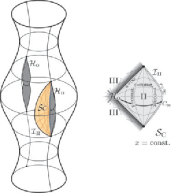
Figure 6: Conformal diagram of the ${t{\text{-}}y}$ section ${\mathcal{S}_{C}}$ not intersecting any horizons outside black holes, and its embedding into the three-dimensional diagram ${\varphi=\text{constant}}$. Such a section of constant $x$ (and $\varphi$) with ${x\in[x_{\mathrm{f}},-{y_{\mathrm{a}}})}$ does not intersect cosmological and acceleration horizons. In contrast to section ${\mathcal{S}_{A}}$ of Fig. 4, section ${\mathcal{S}_{C}}$ does not extend through the whole spacetime, but it can be found near any black hole. Unlike section ${\mathcal{S}_{B}}$ from Fig. 5, it even does not extend between holes of a given pair of black holes. Section ${\mathcal{S}_{C}}$ intersects the infinity in a timelike surface which belongs to domain ${\mathcal{I}}_{\,\mathrm{II}}$ of the conformal infinity, cf. Fig. 10. Notation for infinity, horizons, etc., and the meaning of the shaded area are the same as in Fig. 4.

Finally, for ${x\in[x_{\mathrm{f}},-{y_{\mathrm{a}}})}$ the section ${\mathcal{S}_{C}}$ of constant $x$ extends only to the region II (and regions inside the black hole), and it does not intersect the horizons ${\mathcal{H}}_{\mathrm{a}}$ and ${\mathcal{H}}_{\mathrm{c}}$. The conformal diagram of this type is given in Fig. 6. Section ${\mathcal{S}_{C}}$ intersects the infinity in a timelike surface, and a part of the infinity which can be reached by these sections will be denoted by ${\mathcal{I}}_{\,\mathrm{II}}$, cf. also Fig. 10.

The above described three types of conformal diagrams depicted in Figs. 4–6 have been drawn recently in Dias and Lemos (2003a) (together with special limiting cases ${x=-{y_{\mathrm{c}}}}$ and ${x=-{y_{\mathrm{a}}}}$ which we do not discuss here). Their qualitative dependence on the value of coordinate $x$ has been already noted there but not discussed in more details. Putting all these conformal diagrams together to the single three-dimensional picture shown in Fig. 2(b) elucidates the character of this dependence. Moreover, it clarifies how the timelike infinity ${\mathcal{I}}$ can form a spacelike boundary of a conformal diagram as for section ${\mathcal{S}_{B}}$, Fig. 5 — this spacelike boundary is the intersection of the two timelike hypersurfaces ${\mathcal{I}}$ and ${\mathcal{S}_{B}}$.

In Fig. 2(c) the surfaces ${u=\text{constant}}$ are shown. These null surfaces are formed by null geodesics ${u,\,\zeta=\text{constant}}$ tangent to PND (see Appendix A), and they indicate how the spacetime is covered by Robinson-Trautman coordinates. A surface of constant $u$ reduces to a horizon ${\mathcal{H}}_{\mathrm{a}}$ for ${u=-\infty}$, and to a horizon ${\mathcal{H}}_{\mathrm{o}}$ and ${\mathcal{H}}_{\mathrm{c}}$ for ${u=\infty}$. A connected domain covered by finite values of coordinate $u$ is indicated in Figs. 4–6 by the shaded background. Remaining parts of spacetime have to be covered by different patches of Robinson-Trautman coordinates defined analogously. The domain indicated in figures by a shaded background, covered by a single Robinson-Trautman map, thus reaches up to all types of infinity except to the part ${\mathcal{I}}_{\,{\mathrm{I}^{-}}}$, which is, however, related to the part ${\mathcal{I}}_{\,{\mathrm{I}^{+}}}$ by a simple time reversion. Therefore, we do not loose any substantial information using only this Robinson-Trautman coordinate map.

III Gravitational and electromagnetic fields near ${\mathcal{I}}$

Now we are prepared to discuss radiative properties of the $C$-metric fields near the timelike infinity ${\mathcal{I}}$. As we have already mentioned in Sec. I, following Penrose and Rindler (1986), by radiative field we understand a field with the dominant component having the $1/\eta$ fall-off, calculated in a tetrad parallelly transported along a null geodesic $z{}(\eta)$, $\eta$ being the affine parameter. In the following we derive the characteristic directional pattern of radiation, i.e., the dependence of the radiative component of the fields on the direction along which a given point at the infinity is approached.

We start with a general null geodesics $z(\eta)$ approaching a fixed point $N_{\scriptscriptstyle{\infty}}$ at infinity ${\mathcal{I}}$ as ${\eta\to+\infty}$ (or ${\eta\to-\infty}$). We observe that coordinates ${x,\,y}$, and ${u,\,\zeta}$, as well as metric functions ${F,\,G}$, and $P$, are finite at the point $N_{\scriptscriptstyle{\infty}}$, whereas the affine parameter $\eta$ and the Robinson-Trautman coordinate $r$ go to infinity as the geodesic approaches ${\mathcal{I}}$, cf. Sec. II. We denote the limiting values on ${\mathcal{I}}$ of the coordinates and the metric functions by a subscript “${\scriptscriptstyle{\infty}}$”.

To obtain a more detailed description how $N_{\scriptscriptstyle{\infty}}$ is reached, we have to find the tangent vector of the geodesic,

$$\frac{Dz}{d\eta}=\dot{t}\,{{\boldsymbol{\mathbf{\partial}}}_{t}}+\dot{y}\,{{\boldsymbol{\mathbf{\partial}}}_{y}}+\dot{x}\,{{\boldsymbol{\mathbf{\partial}}}_{x}}+\dot{\varphi}\,{{\boldsymbol{\mathbf{\partial}}}_{\varphi}}{\mbox{\;.}}$$ (17)

As mentioned in Kinnersley and Walker (1970), an explicit form of the tangent vector can be obtained using specific geometrical properties of the $C$-metric (1). The presence of two Killing vectors ${{\boldsymbol{\mathbf{\partial}}}_{t}}$, ${{\boldsymbol{\mathbf{\partial}}}_{\varphi}}$, and of one conformal Killing tensor ${\boldsymbol{\mathbf{Q}}}$ (cf. Sec. II) implies that there exist three constants of motion ${E=-{{\boldsymbol{\mathbf{\partial}}}_{t}}\mathbin{\boldsymbol{\cdot}}\frac{Dz}{d\eta}}$, ${J={{\boldsymbol{\mathbf{\partial}}}_{\varphi}}}\mathbin{\boldsymbol{\cdot}}\frac{Dz}{d\eta}$, and ${Q=\frac{1}{2}\,{\boldsymbol{\mathbf{Q}}}\mspace{0.8mu}(\frac{Dz}{d\eta},\frac{Dz}{d\eta})}$, respectively, for any null geodesic. Namely, we have

$$\begin{gathered}E=\frac{F\dot{t}}{A^{2}(x+y)^{2}}{\mbox{\;,\quad}}J=\frac{G\dot{\varphi}}{A^{2}(x+y)^{2}}{\mbox{\;,}}\\ Q=\frac{F\dot{t}^{2}-F^{-1}\dot{y}^{2}+G^{-1}\dot{x}^{2}+G\dot{\varphi}^{2}}{2A^{4}(x+y)^{4}}{\mbox{\;.}}\end{gathered}$$ (18)

In addition, $\frac{Dz}{d\eta}$ has a null norm

$$-F\dot{t}^{2}+F^{-1}\dot{y}^{2}+G^{-1}\dot{x}^{2}+G\dot{\varphi}^{2}=0{\mbox{\;.}}$$ (19)

The above four equations imply

$$\dot{t} =EA^{2}(x+y)^{2}F^{-1}{\mbox{\;,}} \dot{y} =\epsilon_{y}A^{2}(x+y)^{2}\sqrt{E^{2}-QF}{\mbox{\;,}}$$ (20)

$$\dot{\varphi} =JA^{2}(x+y)^{2}G^{-1}{\mbox{\;,}} \dot{x} =\epsilon_{x}A^{2}(x+y)^{2}\sqrt{QG-J^{2}}{\mbox{\;,}}$$

where ${\epsilon_{y},\epsilon_{x}=\pm 1}$ are the signs of $\dot{y}$ and $\dot{x}$, respectively. The components of the tangent vector $\frac{Dz}{d\eta}$ in the Robinson-Trautman coordinates (7) are thus given by

$$\dot{r} =-\epsilon_{x}A\sqrt{QG-J^{2}}-\epsilon_{y}A\sqrt{E^{2}-QF}{\mbox{\;,}}$$ (21)

$$\dot{u} =\frac{1}{Ar^{2}F}\Bigl{(}\epsilon_{y}\sqrt{E^{2}-QF}+E\Bigr{)}{\mbox{\;,}}$$

$$\dot{\zeta} =\frac{1}{\sqrt{2}r^{2}}\Bigl{(}\epsilon_{y}\sqrt{E^{2}-QF}F^{-1}+EF^{-1}$$

$$\mspace{60.0mu}-\epsilon_{x}\sqrt{QG-J^{2}}G^{-1}-iJG^{-1}\Bigr{)}{\mbox{\;.}}$$

We immediately observe that there exists a family of simple null geodesics $\dot{r}=A\,E$, ${\dot{\zeta}=0=\dot{u}}$, corresponding to the special choice of the constants ${J=0=Q}$, ${\epsilon_{y}=-\operatorname{sgn}E}$. These lie in the planes $x,\varphi=\text{constant}$, cf. (20), and they are considered in Appendix A.

Now, we notice that $\dot{r}$ remains finite at infinity ${\mathcal{I}}$,

$$\dot{r}\approx-\epsilon_{x}A\sqrt{QG_{\scriptscriptstyle{\infty}}-J^{2}}-\epsilon_{y}A\sqrt{E^{2}-QF_{\scriptscriptstyle{\infty}}}\equiv\gamma{\mbox{\;.}}$$ (22)

This means that $r$ and $\eta$ are asymptotically proportional,

$$r\approx\gamma\,\eta{\mbox{\;.}}$$ (23)

We can thus easily obtain the asymptotic behavior of the above tangent vector by expanding expressions (21) in powers of $1/\eta$ (assuming ${\gamma\neq 0}$ because the geodesic approaches infinity). We get

$$\frac{Dz}{d\eta}\approx\frac{1}{\gamma\,\eta^{2}}\,\Bigl{(}r^{2}{{\boldsymbol{\mathbf{\partial}}}_{r}}-c\,{{\boldsymbol{\mathbf{\partial}}}_{\zeta}}-\bar{c}\,{{\boldsymbol{\mathbf{\partial}}}_{\bar{\zeta}}}-d\,{{\boldsymbol{\mathbf{\partial}}}_{u}}\Bigr{)}{\mbox{\;,}}$$ (24)

with the constants ${c\in{\mathbb{C}}}$ and ${d\in{\mathbb{R}}}$ related to the conserved quantities $E,\,J,\,Q$ by

$$c =-\frac{1}{\gamma\sqrt{2}}\Bigl{(}\epsilon_{y}\sqrt{E^{2}-QF_{\scriptscriptstyle{\infty}}}F_{\scriptscriptstyle{\infty}}^{-1}+EF_{\scriptscriptstyle{\infty}}^{-1}$$ (25)

$$\mspace{65.0mu}-\epsilon_{x}\sqrt{QG_{\scriptscriptstyle{\infty}}-J^{2}}G_{\scriptscriptstyle{\infty}}^{-1}-iJG_{\scriptscriptstyle{\infty}}^{-1}\Bigr{)}{\mbox{\;,}}$$

$$d =-\frac{1}{\gamma AF_{\scriptscriptstyle{\infty}}}\Bigl{(}\epsilon_{y}\sqrt{E^{2}-QF_{\scriptscriptstyle{\infty}}}+E\Bigr{)}{\mbox{\;.}}$$

These constants are not independent. In fact, they satisfy the normalization condition (19) which in Robinson-Trautman coordinates asymptotically reads (recall Eqs. (9) and (15))

$$2P_{\scriptscriptstyle{\infty}}^{-2}c\bar{c}+2d+\frac{\Lambda}{3}\,d^{2}=0{\mbox{\;.}}$$ (26)

The expansion (24) of the tangent vector corresponds to the asymptotic form of null geodesics ${z(\eta)}$ near ${\mathcal{I}}$ given by Eq. (23) and

$$\zeta=\zeta_{\scriptscriptstyle{\infty}}+\frac{c}{\gamma\,\eta}+\dots\mbox{\;,\quad}u=u_{\scriptscriptstyle{\infty}}+\frac{d}{\gamma\,\eta}+\cdots{\mbox{\;.}}$$ (27)

The constants $\zeta_{\scriptscriptstyle{\infty}}$, $u_{\scriptscriptstyle{\infty}}$ specify the position at ${\mathcal{I}}$ which particular geodesic (27) is approaching (or from which it is receding), whereas $c$, $d$ represent the (spacetime) direction along which $N_{\scriptscriptstyle{\infty}}$ is reached. The constant $\gamma$ fixes the affine parameter $\eta$. From Eq. (23) we see that if ${\gamma>0}$ then $r$ is growing and geodesics are approaching the infinity for ${\eta\to+\infty}$ — we will denote these as outgoing. On the other hand, when ${\gamma<0}$ then the geodesics approach ${\mathcal{I}}$ (${r\to\infty}$) as ${\eta\to-\infty}$, i.e., the coordinate $r$ is decreasing with a growing $\eta$. The corresponding geodesics are ingoing: they “start” on ${\mathcal{I}}$ and recede from this into finite regions of the spacetime.

Solving the normalization condition (26) we obtain

$$d+\frac{3}{\Lambda}=\epsilon\frac{3}{\Lambda}\,\sqrt{1-\frac{\Lambda}{3}\,\frac{2c\bar{c}}{P_{\scriptscriptstyle{\infty}}^{2}}}{\mbox{\;,}}$$ (28)

where ${\epsilon=\pm 1}$. For any given $c$ there are thus two real values of $d$, according to the sign of $\epsilon$. In fact, the above parameter $\epsilon$ identifies whether the geodesic is future or past oriented. To see this explicitly, let us consider the future-oriented timelike vector ${{\boldsymbol{\mathbf{\partial}}}_{u}}$ near infinity (${{{\boldsymbol{\mathbf{\partial}}}_{u}}\mathbin{\boldsymbol{\cdot}}{{\boldsymbol{\mathbf{\partial}}}_{u}}=-H\approx\frac{\Lambda}{3}\,r^{2}<0}$). The projection of tangent vector (24) onto ${{\boldsymbol{\mathbf{\partial}}}_{u}}$ is, using (28),

$$\frac{Dz}{d\eta}\mathbin{\boldsymbol{\cdot}}{{\boldsymbol{\mathbf{\partial}}}_{u}}\approx-\gamma\,\Big{(}1+\frac{\Lambda}{3}d\Big{)}=-\epsilon\,\gamma\,\sqrt{1-\frac{\Lambda}{3}\,\frac{2c\bar{c}}{P_{\scriptscriptstyle{\infty}}^{2}}}{\mbox{\;.}}$$ (29)

The geodesic is thus future or past oriented when ${\epsilon\,\gamma>0}$ or ${\epsilon\,\gamma<0}$, respectively. Of course, it is physically natural to restrict ourselves to future-oriented geodesics only. Without loss of generality we thus assume the identification

$$\operatorname{sgn}\gamma=\epsilon{\mbox{\;.}}$$ (30)

Consequently, geodesics with ${\epsilon=+1}$ are outgoing (reaching ${\mathcal{I}}$ for ${\eta\to+\infty}$) whereas those with ${\epsilon=-1}$ are ingoing (starting at ${\mathcal{I}}$ for ${\eta\to-\infty}$).

In order to find the radiative behavior of fields near ${\mathcal{I}}$ we have to set up an interpretation tetrad transported parallelly along a general asymptotic null geodesic, and project the Weyl tensor and the tensor of electromagnetic field onto this tetrad. In fact, in the following we will employ several orthonormal and null tetrads which will be distinguished by specific labels in subscript. We denote the vectors of a generic orthonormal tetrad as ${{{\boldsymbol{\mathbf{t}}}},\,{{\boldsymbol{\mathbf{q}}}},\,{{\boldsymbol{\mathbf{r}}}},\,{{\boldsymbol{\mathbf{s}}}}}$, where ${{\boldsymbol{\mathbf{t}}}}$ is a unit timelike vector and the remaining three are spacelike. With this normalized tetrad we associate a null tetrad ${{{\boldsymbol{\mathbf{k}}}},\,{{\boldsymbol{\mathbf{l}}}},\,{{\boldsymbol{\mathbf{m}}}},\,{\bar{{\boldsymbol{\mathbf{m}}}}}}$,

$${{\boldsymbol{\mathbf{k}}}} =\textstyle{\frac{1}{\sqrt{2}}}({{\boldsymbol{\mathbf{t}}}}+{{\boldsymbol{\mathbf{q}}}}){\mbox{\;,\quad}} {{\boldsymbol{\mathbf{l}}}} =\textstyle{\frac{1}{\sqrt{2}}}({{\boldsymbol{\mathbf{t}}}}-{{\boldsymbol{\mathbf{q}}}}){\mbox{\;,}}$$ (31)

$${{\boldsymbol{\mathbf{m}}}} =\textstyle{\frac{1}{\sqrt{2}}}({{\boldsymbol{\mathbf{r}}}}-i\,{{\boldsymbol{\mathbf{s}}}}){\mbox{\;,\quad}} {\bar{{\boldsymbol{\mathbf{m}}}}} =\textstyle{\frac{1}{\sqrt{2}}}({{\boldsymbol{\mathbf{r}}}}+i\,{{\boldsymbol{\mathbf{s}}}}){\mbox{\;,\quad}}$$

such that

$${{\boldsymbol{\mathbf{k}}}}\mathbin{\boldsymbol{\cdot}}{{\boldsymbol{\mathbf{l}}}}=-1{\mbox{\;,\quad}}{{\boldsymbol{\mathbf{m}}}}\mathbin{\boldsymbol{\cdot}}{\bar{{\boldsymbol{\mathbf{m}}}}}=1{\mbox{\;,}}$$ (32)

all other scalar products being zero.

The Weyl tensor is parametrized by five standard complex coefficients $\Psi_{n}$, $n=0,1,2,3,4,$ defined as its specific components with respect to the above null tetrad, see Eq. (75). Similarly, the tensor of electromagnetic field is parametrized by $\Phi_{n}$, $n=0,1,2$, see Eq. (76). The well-known transformation properties of coefficients $\Psi_{n}$ and $\Phi_{n}$ under null rotations, boost, and spatial rotation of the tetrad are summarized in Appendix B.

To define a suitable interpretation tetrad ${{{\boldsymbol{\mathbf{k}}}}_{\mathrm{i}},\,{{\boldsymbol{\mathbf{l}}}}_{\mathrm{i}},{{\boldsymbol{\mathbf{m}}}}_{\mathrm{i}},\,{\bar{{\boldsymbol{\mathbf{m}}}}}_{\mathrm{i}}}$ we need to specify either its initial condition inside the spacetime, or its final condition at timelike infinity ${\mathcal{I}}$, in a comparable way for all geodesics approaching infinity along different directions. We consider geodesics which reach the same point $N_{\scriptscriptstyle{\infty}}$ at ${\mathcal{I}}$, and thus we prescribe the final condition there. We naturally require that the null vector ${{\boldsymbol{\mathbf{k}}}}_{\mathrm{i}}$ is proportional to the tangent vector (24) of the asymptotic null geodesic (27),

$${{\boldsymbol{\mathbf{k}}}}_{\mathrm{i}}\approx\frac{\epsilon}{\gamma}\,\frac{Dz}{d\eta}{\mbox{\;.}}$$ (33)

We wish to compare the radiation for all such null geodesics approaching the given point at ${\mathcal{I}}$, and it is thus necessary to consider a unique and universal normalization of the affine parameter $\eta$, and of the vector ${{\boldsymbol{\mathbf{k}}}}_{\mathrm{i}}$. A natural and also the most convenient choice is to keep the parameter $\gamma$ fixed — see an analogous discussion in Krtouš and Podolský (2003) near Eqs. (5.6) and (5.9). In fact, this is equivalent to fixing the component ${{\boldsymbol{\mathbf{p}}}\mathbin{\boldsymbol{\cdot}}{{\boldsymbol{\mathbf{n}}}}}$ of the 4-momentum ${{\boldsymbol{\mathbf{p}}}=\frac{Dz}{d\eta}}$ at some large value of $r$, i.e. at given the proximity of the conformal infinity.

Following a general framework introduced in Penrose and Rindler (1986), the null vector ${{\boldsymbol{\mathbf{l}}}}_{\mathrm{i}}$ of the interpretation tetrad now can be fixed asymptotically by normalization (32) and the requirement that on ${\mathcal{I}}$ the vector ${{\boldsymbol{\mathbf{n}}}}$ normal to the infinity belongs to ${{\boldsymbol{\mathbf{k}}}}_{\mathrm{i}}{\text{-}}{{\boldsymbol{\mathbf{l}}}}_{\mathrm{i}}$ plane. Obviously, the direction of ${{\boldsymbol{\mathbf{l}}}}_{\mathrm{i}}$ at a point $N_{\scriptscriptstyle{\infty}}$ on ${\mathcal{I}}$ thus uniquely depends on the choice of the particular null geodesic (27) approaching infinity, i.e., on the specific vector ${{\boldsymbol{\mathbf{k}}}}_{\mathrm{i}}$. Remaining vectors ${{{\boldsymbol{\mathbf{m}}}}_{\mathrm{i}},\,{\bar{{\boldsymbol{\mathbf{m}}}}}_{\mathrm{i}}}$ cannot be prescribed canonically — there is a freedom in choice of their phase factor (a rotation in the transverse ${{{\boldsymbol{\mathbf{m}}}}_{\mathrm{i}}{\text{-}}{\bar{{\boldsymbol{\mathbf{m}}}}}_{\mathrm{i}}}$ plane). Therefore, we have to find such physical quantities which are invariant under this freedom. Obviously, the moduli $|\Psi_{n}|$ and $|\Phi_{n}|$ of the fields at ${\mathcal{I}}$ are independent of the specific choice of the vectors ${{{\boldsymbol{\mathbf{m}}}}_{\mathrm{i}},\,{\bar{{\boldsymbol{\mathbf{m}}}}}_{\mathrm{i}}}$.

To derive the field components in the above-defined interpretation tetrad we start with the simple Robinson-Trautman null tetrad ${{{\boldsymbol{\mathbf{k}}}}_{\scriptscriptstyle\mathrm{RT}},\,{{\boldsymbol{\mathbf{l}}}}_{\scriptscriptstyle\mathrm{RT}},\,{{\boldsymbol{\mathbf{m}}}}_{\scriptscriptstyle\mathrm{RT}},\,{\bar{{\boldsymbol{\mathbf{m}}}}}_{\scriptscriptstyle\mathrm{RT}}}$ (see, e.g., Kramer et al. (1980)) naturally adapted to the Robinson-Trautman coordinates (8)

$${{\boldsymbol{\mathbf{k}}}}_{\scriptscriptstyle\mathrm{RT}} =\;{{\boldsymbol{\mathbf{\partial}}}_{r}}{\mbox{\;,}}$$ (34)

$${{\boldsymbol{\mathbf{l}}}}_{\scriptscriptstyle\mathrm{RT}} =-\textstyle{\frac{1}{2}}H\,{{\boldsymbol{\mathbf{\partial}}}_{r}}+{{\boldsymbol{\mathbf{\partial}}}_{u}}{\mbox{\;,}}$$

$${{\boldsymbol{\mathbf{m}}}}_{\scriptscriptstyle\mathrm{RT}} =\frac{P}{r}\,{{\boldsymbol{\mathbf{\partial}}}_{\bar{\zeta}}}{\mbox{\;,}}$$

$${\bar{{\boldsymbol{\mathbf{m}}}}}_{\scriptscriptstyle\mathrm{RT}} =\frac{P}{r}\,{{\boldsymbol{\mathbf{\partial}}}_{\zeta}}{\mbox{\;.}}$$

Note that the vector ${{\boldsymbol{\mathbf{k}}}}_{\scriptscriptstyle\mathrm{RT}}$ is oriented along the double degenerate principal null direction ${{\boldsymbol{\mathbf{k}}}}_{1}$, cf. Eq. (65). In this tetrad the only nontrivial components $\Psi^{{\scriptscriptstyle\mathrm{RT}}}_{n}$ and $\Phi^{{\scriptscriptstyle\mathrm{RT}}}_{n}$, which represent the gravitational and electromagnetic fields, are

$$\begin{gathered}\Psi^{{\scriptscriptstyle\mathrm{RT}}}_{2}=-\Bigl{(}m+2\,e^{2}A\,x-\frac{e^{2}}{r}\Bigr{)}\,\frac{1}{r^{3}}{\mbox{\;,}}\\ \Psi^{{\scriptscriptstyle\mathrm{RT}}}_{3}=-\frac{3}{\sqrt{2}}\,\frac{A\,r}{P}\,\Psi^{{\scriptscriptstyle\mathrm{RT}}}_{2}{\mbox{\;,\quad}}\Psi^{{\scriptscriptstyle\mathrm{RT}}}_{4}=3\,\frac{A^{2}\,r^{2}}{P^{2}}\,\Psi^{{\scriptscriptstyle\mathrm{RT}}}_{2}{\mbox{\;,}}\\ \Phi^{{\scriptscriptstyle\mathrm{RT}}}_{1}=-\frac{e}{2\,r^{2}}{\mbox{\;,\quad}}\Phi^{{\scriptscriptstyle\mathrm{RT}}}_{2}=-\sqrt{2}\,\frac{A\,r}{P}\,\Phi^{{\scriptscriptstyle\mathrm{RT}}}_{1}{\mbox{\;.}}\end{gathered}$$ (35)

The interpretation tetrad ${{{\boldsymbol{\mathbf{k}}}}_{\mathrm{i}},\,{{\boldsymbol{\mathbf{l}}}}_{\mathrm{i}},{{\boldsymbol{\mathbf{m}}}}_{\mathrm{i}},\,{\bar{{\boldsymbol{\mathbf{m}}}}}_{\mathrm{i}}}$ can be obtained by performing two subsequent null rotations and a boost of this Robinson-Trautman null tetrad (34). We first apply (80), then (77), and finally (83) of Appendix B with the parameters

$$K =-\Big{(}1+\frac{\Lambda}{6}d\Big{)}^{-1}\frac{c}{P\,r}{\mbox{\;,}}$$ (36)

$$L =\frac{\Lambda}{6}\frac{c\,r}{P}{\mbox{\;,}}$$

$$B =\epsilon\,\Big{(}1+\frac{\Lambda}{6}d\Big{)}{\mbox{\;,\quad}}\quad\Phi=0{\mbox{\;.}}$$

The resulting null tetrad, using relation (26), then takes the following asymptotic form as ${\eta\to\epsilon\infty}$,

$${{\boldsymbol{\mathbf{k}}}}_{\mathrm{i}} \approx\epsilon\frac{1}{\gamma^{2}\eta^{2}}\,\left(r^{2}{{\boldsymbol{\mathbf{\partial}}}_{r}}-c\,{{\boldsymbol{\mathbf{\partial}}}_{\zeta}}-\bar{c}\,{{\boldsymbol{\mathbf{\partial}}}_{\bar{\zeta}}}-d\,{{\boldsymbol{\mathbf{\partial}}}_{u}}\right){\mbox{\;,}}$$ (37)

$${{\boldsymbol{\mathbf{l}}}}_{\mathrm{i}} \approx\epsilon\frac{\Lambda}{6}\,\left(r^{2}{{\boldsymbol{\mathbf{\partial}}}_{r}}+c\,{{\boldsymbol{\mathbf{\partial}}}_{\zeta}}+\bar{c}\,{{\boldsymbol{\mathbf{\partial}}}_{\bar{\zeta}}}+\Big{(}d+\frac{6}{\Lambda}\Big{)}\,{{\boldsymbol{\mathbf{\partial}}}_{u}}\right){\mbox{\;,}}$$

$${{\boldsymbol{\mathbf{m}}}}_{\mathrm{i}} \approx\frac{P_{\scriptscriptstyle{\infty}}}{\gamma\,\eta}\left(\,\frac{\Lambda}{6}\frac{c\,d}{\bar{c}}\,{{\boldsymbol{\mathbf{\partial}}}_{\zeta}}+\Big{(}1+\frac{\Lambda}{6}d\Big{)}\,{{\boldsymbol{\mathbf{\partial}}}_{\bar{\zeta}}}-\frac{c}{P_{\scriptscriptstyle{\infty}}^{2}}\,{{\boldsymbol{\mathbf{\partial}}}_{u}}\right){\mbox{\;,}}$$

$${\bar{{\boldsymbol{\mathbf{m}}}}}_{\mathrm{i}} \approx\frac{P_{\scriptscriptstyle{\infty}}}{\gamma\,\eta}\left(\,\Big{(}1+\frac{\Lambda}{6}d\Big{)}\,{{\boldsymbol{\mathbf{\partial}}}_{\zeta}}+\frac{\Lambda}{6}\frac{\bar{c}\,d}{c}\,{{\boldsymbol{\mathbf{\partial}}}_{\bar{\zeta}}}-\frac{\bar{c}}{P_{\scriptscriptstyle{\infty}}^{2}}\,{{\boldsymbol{\mathbf{\partial}}}_{u}}\right){\mbox{\;.}}$$

The above vector ${{\boldsymbol{\mathbf{k}}}}_{\mathrm{i}}$ is indeed obviously tangent to a general asymptotic null geodesics (27), and satisfies the condition (33). Moreover, the normal ${{\boldsymbol{\mathbf{n}}}}$ to ${\mathcal{I}}$, cf. Eq. (16), belongs to the plane spanned by the two null vectors ${{\boldsymbol{\mathbf{k}}}}_{\mathrm{i}}$ and ${{\boldsymbol{\mathbf{l}}}}_{\mathrm{i}}$, as required,

$${{\boldsymbol{\mathbf{n}}}}\approx\frac{\epsilon}{\sqrt{2}}\Bigl{(}\,\sqrt{-\frac{\Lambda}{6}}\;\gamma\,\eta\;{{\boldsymbol{\mathbf{k}}}}_{\mathrm{i}}-\sqrt{-\frac{6}{\Lambda}}\;\frac{1}{\gamma\,\eta}\;{{\boldsymbol{\mathbf{l}}}}_{\mathrm{i}}\,\Bigr{)}{\mbox{\;.}}$$ (38)

Notice that the projection of ${{\boldsymbol{\mathbf{k}}}}_{\mathrm{i}}$ on ${{\boldsymbol{\mathbf{n}}}}$ is

$${{\boldsymbol{\mathbf{k}}}}_{\mathrm{i}}\mathbin{\boldsymbol{\cdot}}{{\boldsymbol{\mathbf{n}}}}\approx\frac{\epsilon}{\gamma\,\eta}\sqrt{-\frac{3}{\Lambda}}{\mbox{\;.}}$$ (39)

For outgoing geodesics (${\epsilon=+1}$, ${\eta\to+\infty}$) we indeed obtain ${{{\boldsymbol{\mathbf{k}}}}_{\mathrm{i}}\mathbin{\boldsymbol{\cdot}}{{\boldsymbol{\mathbf{n}}}}>0}$, whereas for ingoing ones (${\epsilon=-1}$, ${\eta\to-\infty}$) there is ${{{\boldsymbol{\mathbf{k}}}}_{\mathrm{i}}\mathbin{\boldsymbol{\cdot}}{{\boldsymbol{\mathbf{n}}}}<0}$.

Therefore, the tetrad (37) is exactly the interpretation tetrad suitable for analysis of the behavior of fields close to infinity ${\mathcal{I}}$. As seen above, the Lorentz transformations from the tetrad (34) to (37) are given by two subsequent null rotations and the boost with the parameters (36). Starting with the components (35) in the Robinson-Trautman frame we thus obtain, using Eqs. (81), (78), (84) and (82), (79), (85), the asymptotic form of the leading terms of gravitational and electromagnetic fields

$$\Psi^{{\mathrm{i}}}_{4} \approx-\frac{3(m+2e^{2}A\,x_{\scriptscriptstyle{\infty}})}{\gamma\,\eta\,P_{\scriptscriptstyle{\infty}}^{2}}\,\left[\,A\left(1+{\frac{\Lambda}{6}}\,d\right)-\frac{\Lambda\,\bar{c}}{3\sqrt{2}}\,\right]^{2}{\mbox{\;,}}$$

$$\Phi^{{\mathrm{i}}}_{2} \approx\ \frac{\epsilon\,e}{\sqrt{2}\,\gamma\,\eta\,P_{\scriptscriptstyle{\infty}}}\,\left[\,A\left(1+{\frac{\Lambda}{6}}\,d\right)-\frac{\Lambda\,\bar{c}}{3\sqrt{2}}\,\right]{\mbox{\;,}}$$ (40)

where $x_{\scriptscriptstyle{\infty}}$ is the coordinate of the point $N_{\scriptscriptstyle{\infty}}$ related to the coordinates $\zeta_{\scriptscriptstyle{\infty}},u_{\scriptscriptstyle{\infty}}$ by Eq. (11). The other terms decrease faster in accordance with the well-known peeling behavior, which is a consequence of the boost contained in (38) that is infinite on ${\mathcal{I}}$, cf. Penrose and Rindler (1986). Notice also that the square of $\Phi^{{\mathrm{i}}}_{2}$ gives the modulus of the Poynting vector, $4\pi\left\lvert{\boldsymbol{\mathbf{S}}}_{\mathrm{i}}\right\rvert\approx\left\lvert\Phi^{{\mathrm{i}}}_{2}\right\rvert^{2}$, defined in the interpretation tetrad (37). Interestingly, the dependence of ${\left\lvert\Psi^{{\mathrm{i}}}_{4}\right\rvert}$ and ${\left\lvert\Phi^{{\mathrm{i}}}_{2}\right\rvert^{2}}$ on the direction along which the point $N_{\scriptscriptstyle{\infty}}$ at infinity ${\mathcal{I}}$ is approached is exactly the same.

Expressions (40) are (formally) identical to Eqs. (6.16) of Krtouš and Podolský (2003) in which radiation in the $C$-metric spacetime with ${\Lambda>0}$ was investigated. Interestingly enough, one can also directly set ${\Lambda=0}$. The directional dependence given by the parameters $c$ and $d$ vanishes in this limit (since ${{\boldsymbol{\mathbf{l}}}}_{\mathrm{i}}$ becomes independent of ${{\boldsymbol{\mathbf{k}}}}_{\mathrm{i}}$) and formulas (40) can be compared with the results obtained in classic work Kinnersley and Walker (1970) (see also Farhoosh and Zimmerman (1979)) for accelerated black holes in asymptotically flat spacetime.

Nevertheless, the physical and geometrical meanings of Eqs. (40) is very different now since new interesting and specific features occur for the ${\Lambda<0}$ case. The following sections will be devoted to deeper description and analysis of the above result.

IV Parametrizations of the null direction at ${\mathcal{I}}$

For a physical understanding of expressions (40), as well as for explicit demonstration of fundamental differences between radiation generated by accelerated black holes in spacetimes with ${\Lambda>0}$ and ${\Lambda<0}$, we introduce more convenient parametrizations of the direction ${{\boldsymbol{\mathbf{k}}}}_{\mathrm{i}}$ along which the infinity ${\mathcal{I}}$ — now timelike — is approached. To parametrize this radiation direction we first choose a suitable reference tetrad ${{{\boldsymbol{\mathbf{t}}}}_{\mathrm{o}},\,{{\boldsymbol{\mathbf{q}}}}_{\mathrm{o}},\,{{\boldsymbol{\mathbf{r}}}}_{\mathrm{o}},\,{{\boldsymbol{\mathbf{s}}}}_{\mathrm{o}}}$ on ${\mathcal{I}}$ which is orthonormal, adapted to the infinity,

$${{\boldsymbol{\mathbf{q}}}}_{\mathrm{o}}={{\boldsymbol{\mathbf{n}}}}{\mbox{\;,}}$$ (41)

and with ${{\boldsymbol{\mathbf{t}}}}_{\mathrm{o}}$ future oriented. Otherwise the tetrad can be chosen arbitrarily. A natural choice is to consider a tetrad closely related to the Robinson-Trautman tetrad (34), namely,

$${{\boldsymbol{\mathbf{k}}}}_{\mathrm{o}}=\sqrt{\frac{H}{2}}\;{{\boldsymbol{\mathbf{k}}}}_{\scriptscriptstyle\mathrm{RT}}{\mbox{\;,}}\quad{{\boldsymbol{\mathbf{l}}}}_{\mathrm{o}}=\sqrt{\frac{2}{H}}\;{{\boldsymbol{\mathbf{l}}}}_{\scriptscriptstyle\mathrm{RT}}{\mbox{\;,}}\quad{{\boldsymbol{\mathbf{m}}}}_{\mathrm{o}}={{\boldsymbol{\mathbf{m}}}}_{\scriptscriptstyle\mathrm{RT}}{\mbox{\;,}}$$ (42)

so that (cf. Eq. (31))

$${{\boldsymbol{\mathbf{\partial}}}_{u}} =\sqrt{H}\;{{\boldsymbol{\mathbf{t}}}}_{\mathrm{o}}{\mbox{\;,}}$$ (43)

$${{\boldsymbol{\mathbf{\partial}}}_{r}} =\frac{1}{\sqrt{H}}\,\left(\,{{\boldsymbol{\mathbf{t}}}}_{\mathrm{o}}+{{\boldsymbol{\mathbf{q}}}}_{\mathrm{o}}\,\right){\mbox{\;,}}$$

$${{\boldsymbol{\mathbf{\partial}}}_{\zeta}} =\frac{1}{\sqrt{2}}\,\frac{r}{P}\,\left(\,{{\boldsymbol{\mathbf{r}}}}_{\mathrm{o}}+i\,{{\boldsymbol{\mathbf{s}}}}_{\mathrm{o}}\,\right){\mbox{\;.}}$$

The null direction ${{\boldsymbol{\mathbf{k}}}}_{\mathrm{i}}$ can be obtained (up to normalization) from the above reference vector ${{\boldsymbol{\mathbf{k}}}}_{\mathrm{o}}$ by a null rotation (80), and thus it can be parametrized by a complex parameter $R$ as

$${{\boldsymbol{\mathbf{k}}}}_{\mathrm{i}}\propto{{\boldsymbol{\mathbf{k}}}}_{\mathrm{o}}+\bar{R}\,{{\boldsymbol{\mathbf{m}}}}_{\mathrm{o}}+R\,{\bar{{\boldsymbol{\mathbf{m}}}}}_{\mathrm{o}}+R\bar{R}\,{{\boldsymbol{\mathbf{l}}}}_{\mathrm{o}}{\mbox{\;.}}$$ (44)

Comparing this expression with Eq. (37) we can relate $R$ to the parameters $c$ and $d$,

$$c =-\sqrt{-\frac{6}{\Lambda}}\,P_{\scriptscriptstyle{\infty}}\,\frac{R}{1-\left\lvert R\right\rvert^{2}}{\mbox{\;,}}$$ (45)

$$d =\frac{6}{\Lambda}\,\frac{\left\lvert R\right\rvert^{2}}{1-\left\lvert R\right\rvert^{2}}{\mbox{\;.}}$$

Now we may rewrite the directional pattern (40) in terms of the parameter $R$. First, recall that there is no canonical way how to choose the phase of the transverse null vectors ${{{\boldsymbol{\mathbf{m}}}}_{\mathrm{i}},\,{\bar{{\boldsymbol{\mathbf{m}}}}}_{\mathrm{i}}}$. Therefore, invariant information independent of a choice of the interpretation tetrad is contained only in the moduli of fields components. Substituting relations (45) into expressions (40) we obtain

$$\left\lvert\Psi^{{\mathrm{i}}}_{4}\right\rvert \approx\frac{3A^{2}(m+2e^{2}A\,x_{\scriptscriptstyle{\infty}})}{\gamma\,\eta\,P_{\scriptscriptstyle{\infty}}^{2}}\,\frac{\left\lvert 1-R_{1}\bar{R}\right\rvert^{2}\left\lvert 1-R_{2}\bar{R}\right\rvert^{2}}{\bigl{(}1-\left\lvert R\right\rvert^{2}\bigr{)}^{2}}{\mbox{\;,}}$$ (46)

$$\left\lvert\Phi^{{\mathrm{i}}}_{2}\right\rvert \approx\frac{\left\lvert e\right\rvert A}{\sqrt{2}\,\gamma\,\eta\,P_{\scriptscriptstyle{\infty}}}\,\frac{\left\lvert 1-R_{1}\bar{R}\right\rvert\left\lvert 1-R_{2}\bar{R}\right\rvert}{\bigl{\lvert}1-\left\lvert R\right\rvert^{2}\bigr{\rvert}}{\mbox{\;,}}$$

where

$$R_{1}=0{\mbox{\;,\quad}}R_{2}=\sqrt{-\frac{\Lambda}{3}}\,\frac{\,P_{\scriptscriptstyle{\infty}}}{A}{\mbox{\;.}}$$ (47)

We have introduced here not only $R_{2}$ but also a “superfluous” parameter ${R_{1}=0}$. This is motivated by a general result Krtouš and Podolský concerning an asymptotic structure of the fields when ${\Lambda<0}$. In fact, the real parameters $R_{1}$, $R_{2}$ have an important physical meaning — they represent double-degenerate principal null directions (PNDs) ${{\boldsymbol{\mathbf{k}}}}_{1}$ and ${{\boldsymbol{\mathbf{k}}}}_{2}$ (cf. Eq. (5)) at the infinity ${\mathcal{I}}$. Indeed, the specific complex parameter $R$ representing a PND with respect to the reference tetrad has to satisfy quartic equation ${\Psi_{0}=0}$ (see, e.g., Kramer et al. (1980)), i.e., using Eq. (81),

$$R^{4}\Psi^{{\mathrm{o}}}_{4}+4R^{3}\Psi^{{\mathrm{o}}}_{3}+6R^{2}\Psi^{{\mathrm{o}}}_{2}+4R\,\Psi^{{\mathrm{o}}}_{1}+\Psi^{{\mathrm{o}}}_{0}=0{\mbox{\;.}}$$ (48)

This, in view of (42), (84), and (35), asymptotically reduces exactly to

$$(R-R_{1})^{2}(R-R_{2})^{2}=0{\mbox{\;.}}$$ (49)

Therefore, the first double-degenerate PND ${{\boldsymbol{\mathbf{k}}}}_{1}$ is indeed given by ${R=R_{1}}$, whereas the second one, ${{\boldsymbol{\mathbf{k}}}}_{2}$, is given by ${R=R_{2}}$.

Instead of using the complex parameter $R$ for identification of the null direction ${{\boldsymbol{\mathbf{k}}}}_{\mathrm{i}}$ we can introduce two real parameters with an obvious geometrical meaning. First, we perform a normalized projection of the null vector ${{\boldsymbol{\mathbf{k}}}}_{\mathrm{i}}$ onto ${\mathcal{I}}$, defining thus the unit timelike vector ${{\boldsymbol{\mathbf{t}}}}_{\mathrm{b}}$ tangent to the infinity:

$${{\boldsymbol{\mathbf{t}}}}_{\mathrm{b}}=\frac{{{\boldsymbol{\mathbf{k}}}}_{\mathrm{i}}-({{\boldsymbol{\mathbf{k}}}}_{\mathrm{i}}\mathbin{\boldsymbol{\cdot}}{{\boldsymbol{\mathbf{n}}}})\,{{\boldsymbol{\mathbf{n}}}}}{\left\lvert{{\boldsymbol{\mathbf{k}}}}_{\mathrm{i}}\mathbin{\boldsymbol{\cdot}}{{\boldsymbol{\mathbf{n}}}}\right\rvert}{\mbox{\;.}}$$ (50)

Then ${{\boldsymbol{\mathbf{t}}}}_{\mathrm{b}}$ represents the radiation direction along ${\mathcal{I}}$ corresponding to the null vector ${{{\boldsymbol{\mathbf{k}}}}_{\mathrm{i}}\propto\,{{\boldsymbol{\mathbf{t}}}}_{\mathrm{b}}+\epsilon\,{{\boldsymbol{\mathbf{n}}}}}$. We can characterize ${{\boldsymbol{\mathbf{t}}}}_{\mathrm{b}}$ (and thus ${{\boldsymbol{\mathbf{k}}}}_{\mathrm{i}}$) with respect to the reference tetrad as

$${{\boldsymbol{\mathbf{t}}}}_{\mathrm{b}}=\cosh\psi\;{{\boldsymbol{\mathbf{t}}}}_{\mathrm{o}}+\sinh\psi\,(\cos\phi\;{{\boldsymbol{\mathbf{r}}}}_{\mathrm{o}}+\sin\phi\;{{\boldsymbol{\mathbf{s}}}}_{\mathrm{o}}){\mbox{\;.}}$$ (51)

The parameters ${\psi,\phi}$ are pseudo-spherical coordinates, ${\psi\in[0,\infty)}$ corresponding to a boost, and ${\phi\in[0,2\pi)}$ being an angle. Their geometric meaning is visualized in Fig. 7. However, these parameters do not specify the null direction ${{\boldsymbol{\mathbf{k}}}}_{\mathrm{i}}$ uniquely — there always exists one ingoing and one outgoing null direction with the same parameters $\psi$ and $\phi$, which are distinguished by $\epsilon$.

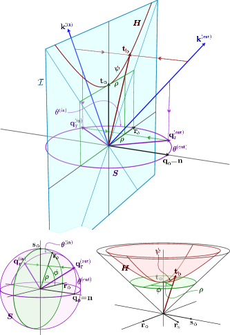
Figure 7: Parametrizations of a null direction at timelike infinity ${\mathcal{I}}$. All null directions at a point $N_{\scriptscriptstyle{\infty}}\in{\mathcal{I}}$ can be characterized by a future oriented null vector ${{\boldsymbol{\mathbf{k}}}}$. According to their orientation ${\epsilon=\operatorname{sgn}({{\boldsymbol{\mathbf{k}}}}\mathbin{\boldsymbol{\cdot}}{{\boldsymbol{\mathbf{n}}}})}$ with respect to ${\mathcal{I}}$, these can be divided into outgoing and ingoing families — see, e.g., vectors ${{\boldsymbol{\mathbf{k}}}}^{\mathrm{(out)}}$ and ${{\boldsymbol{\mathbf{k}}}}^{\mathrm{(in)}}$ in the figure. (Special null directions tangent to ${\mathcal{I}}$ will not be discussed here.) The null direction is parametrized by a boost $\psi$ and an angle $\phi$, or alternatively by spherical angles ${\theta,\,\phi}$. These parametrizations are defined with respect to the reference tetrad ${{{\boldsymbol{\mathbf{t}}}}_{\mathrm{o}},\,{{\boldsymbol{\mathbf{q}}}}_{\mathrm{o}},\,{{\boldsymbol{\mathbf{r}}}}_{\mathrm{o}},\,{{\boldsymbol{\mathbf{s}}}}_{\mathrm{o}}}$. In the top diagram the vectors ${{{\boldsymbol{\mathbf{t}}}}_{\mathrm{o}},\,{{\boldsymbol{\mathbf{q}}}}_{\mathrm{o}},\,{{\boldsymbol{\mathbf{r}}}}_{\phi}}$ (where ${{{\boldsymbol{\mathbf{r}}}}_{\phi}=\cos\phi\,{{\boldsymbol{\mathbf{r}}}}_{\mathrm{o}}+\sin\phi\,{{\boldsymbol{\mathbf{s}}}}_{\mathrm{o}}}$) are depicted, the remaining spatial direction ${{\boldsymbol{\mathbf{s}}}}_{\phi}$ is suppressed. In the bottom left diagram the timelike direction ${{\boldsymbol{\mathbf{t}}}}_{\mathrm{o}}$ is suppressed and all spatial directions are drawn. Finally, in the bottom right diagram the spatial direction ${{{\boldsymbol{\mathbf{q}}}}_{\mathrm{o}}={{\boldsymbol{\mathbf{n}}}}}$ normal to ${\mathcal{I}}$ is omitted. The parameters ${\psi,\,\phi}$ specify the normalized orthogonal projection ${{\boldsymbol{\mathbf{t}}}}_{\mathrm{b}}$ (Eq. (50)) of the null vector ${{\boldsymbol{\mathbf{k}}}}$ onto ${\mathcal{I}}$ by Eq. (51). All possible ${{\boldsymbol{\mathbf{t}}}}_{\mathrm{b}}$ form a two-dimensional hyperboloid $\boldsymbol{H}$ drawn in the bottom right diagram. This hyperboloid can be radially projected onto a two-dimensional disk tangent to the vertex of the hyperboloid given by ${{\boldsymbol{\mathbf{t}}}}_{\mathrm{o}}$. The disk can be parametrized by radial coordinate ${\rho=\tanh\psi}$, and angle $\phi$. Alternatively, the null direction can be characterized by the normalized spatial projection ${{\boldsymbol{\mathbf{q}}}}_{\mathrm{r}}$ (Eq. (57)) of the null vector ${{\boldsymbol{\mathbf{k}}}}$ into the 3-space orthogonal to ${{\boldsymbol{\mathbf{t}}}}_{\mathrm{o}}$. The projection ${{\boldsymbol{\mathbf{q}}}}_{\mathrm{r}}$ can be parametrized by spherical angles ${\theta,\,\phi}$ with respect to the reference tetrad, see Eq. (58). All spatial projections ${{\boldsymbol{\mathbf{q}}}}_{\mathrm{r}}$ form a two-dimensional sphere $\boldsymbol{S}$ shown in the bottom left. This sphere can be orthogonally projected onto ${\mathcal{I}}$, where it again forms a two-dimensional disk parametrized by ${\rho=\sin\theta}$, and $\phi$, cf. Eq. (59).

Substituting Eq. (44) into Eq. (50) and comparing with Eq. (51) we can express $\psi$ and $\phi$ in terms of $R$ as

$$\tanh\psi=\frac{2\left\lvert R\right\rvert}{1+\left\lvert R\right\rvert^{2}}{\mbox{\;,\quad}}\phi=-\arg R{\mbox{\;.}}$$ (52)

Observing that the sign of the expression ${1-\left\lvert R\right\rvert^{2}}\propto{{{\boldsymbol{\mathbf{k}}}}_{\mathrm{i}}\mathbin{\boldsymbol{\cdot}}{{\boldsymbol{\mathbf{n}}}}}$ determines whether ${{\boldsymbol{\mathbf{k}}}}_{\mathrm{i}}$ is ingoing or outgoing, i.e.,

$$\epsilon=\operatorname{sgn}(1-\left\lvert R\right\rvert^{2}){\mbox{\;,}}$$ (53)

we can write down the inverse relations,

$$R=\begin{cases}{\displaystyle\tanh\frac{\psi}{2}\;\exp(-i\phi)}&\text{for ${{\boldsymbol{\mathbf{k}}}}_{\mathrm{i}}$ outgoing (${\epsilon\!=\!+1}$)}{\mbox{\;,}\vspace*{6pt}}\\ {\displaystyle\coth\frac{\psi}{2}\;\exp(-i\phi)}&\text{for ${{\boldsymbol{\mathbf{k}}}}_{\mathrm{i}}$ ingoing (${\epsilon\!=\!-1}$)}{\mbox{\;,}}\end{cases}$$ (54)

and also the relations to the parameters $c$ and $d$,

$$-\epsilon\sqrt{-\frac{\Lambda}{6}}\,\frac{2\bar{c}}{P_{\scriptscriptstyle{\infty}}}=\sinh\psi\exp(i\phi){\mbox{\;,\quad}}\epsilon\Big{(}1+\frac{\Lambda}{3}\,d\Big{)}=\cosh\psi{\mbox{\;.}}$$ (55)

Substituting from (55) into (40) we obtain

$$\left\lvert\Psi^{{\mathrm{i}}}_{4}\right\rvert \approx\frac{\left\lvert\Lambda\right\rvert}{4}\frac{(m+2e^{2}A\,x_{\scriptscriptstyle{\infty}})}{\gamma\,\eta}$$ (56)

$$\quad\times\,\left\lvert R_{2}^{-1}\,(1+\epsilon\cosh\psi)-\epsilon\sinh\psi\,\exp(i\phi)\right\rvert^{2}{\mbox{\;,}}$$

$$\left\lvert\Phi^{{\mathrm{i}}}_{2}\right\rvert \approx\sqrt{\frac{\left\lvert\Lambda\right\rvert}{24}}\,\frac{|e|}{\gamma\,\eta}$$

$$\quad\times\,\left\lvert R_{2}^{-1}\,(1+\epsilon\cosh\psi)-\epsilon\sinh\psi\,\exp(i\phi)\right\rvert{\mbox{\;.}}$$

The dependence of the fields on the parameters $\psi$ and $\phi$ is shown in Fig. 8.

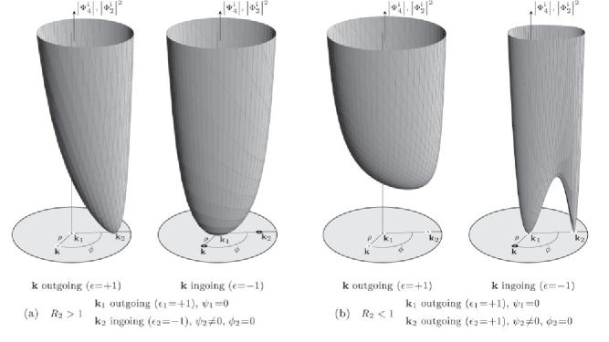
Figure 8: Possible directional patterns of radiation (56) [or, equivalently, (46), (61)] which express the magnitude of the leading terms of gravitational or electromagnetic fields as a function of a direction from which the point $N_{\scriptscriptstyle{\infty}}$ at infinity ${\mathcal{I}}$ is approached. The corresponding outgoing (${\epsilon=+1}$, small white spot) or ingoing (${\epsilon=-1}$, black spot) null geodesic with a tangent vector ${{\boldsymbol{\mathbf{k}}}}$ are parametrized by ${\rho=\tanh\psi}$ and ${\phi}$, cf. Fig. 7. The patterns (a) apply to points $N_{\scriptscriptstyle{\infty}}$ in which the double degenerate PND ${{\boldsymbol{\mathbf{k}}}}_{1}$ (white spot) is oriented outwards from the universe whereas ${{\boldsymbol{\mathbf{k}}}}_{2}$ (black spot) inside it. The patterns (b) apply to points in which both the PNDs are outgoing. The pattern (b) would also apply for points where both PNDs are ingoing, only with exchanged words “ingoing” and “outgoing”. The radiation completely vanishes along directions which are exactly mirrored of the PNDs, with respect to ${\mathcal{I}}$.

There exists yet another natural possibility how to characterize the null direction at the infinity. Instead of decomposing the propagation vector ${{\boldsymbol{\mathbf{k}}}}_{\mathrm{i}}$ into the component normal to ${\mathcal{I}}$ and the transverse timelike vector ${{\boldsymbol{\mathbf{t}}}}_{\mathrm{b}}$ tangent to ${\mathcal{I}}$, we may alternatively consider its normalized spatial projection ${{\boldsymbol{\mathbf{q}}}}_{\mathrm{r}}$, where by the spatial projection we mean a projection to a suitable three-dimensional space, say that orthogonal to ${{\boldsymbol{\mathbf{t}}}}_{\mathrm{o}}$ (see Fig. 7). This spatial propagation vector

$${{\boldsymbol{\mathbf{q}}}}_{\mathrm{r}}=\frac{{{\boldsymbol{\mathbf{k}}}}_{\mathrm{i}}+({{\boldsymbol{\mathbf{k}}}}_{\mathrm{i}}\mathbin{\boldsymbol{\cdot}}{{\boldsymbol{\mathbf{t}}}}_{\mathrm{o}})\,{{\boldsymbol{\mathbf{t}}}}_{\mathrm{o}}}{|{{\boldsymbol{\mathbf{k}}}}_{\mathrm{i}}\mathbin{\boldsymbol{\cdot}}{{\boldsymbol{\mathbf{t}}}}_{\mathrm{o}}|}{\mbox{\;,}}$$ (57)

such that ${{{\boldsymbol{\mathbf{k}}}}_{\mathrm{i}}\propto{{\boldsymbol{\mathbf{t}}}}_{\mathrm{o}}+{{\boldsymbol{\mathbf{q}}}}_{\mathrm{r}}}$, is naturally characterized by spherical angles $\theta$ and $\phi$ with respect to the spatial vectors ${{{\boldsymbol{\mathbf{q}}}}_{\mathrm{o}},\,{{\boldsymbol{\mathbf{r}}}}_{\mathrm{o}},\,{{\boldsymbol{\mathbf{s}}}}_{\mathrm{o}}}$ of the reference tetrad, namely

$${{\boldsymbol{\mathbf{q}}}}_{\mathrm{r}}=\cos\theta\;{{\boldsymbol{\mathbf{q}}}}_{\mathrm{o}}+\sin\theta\,(\cos\phi\;{{\boldsymbol{\mathbf{r}}}}_{\mathrm{o}}+\sin\phi\;{{\boldsymbol{\mathbf{s}}}}_{\mathrm{o}}){\mbox{\;.}}$$ (58)

Obviously, this is more convenient for a unified description of both outgoing (${\epsilon=+1}$) and ingoing (${\epsilon=-1}$) null geodesics. The former are parametrized by ${\theta\in[0,\frac{\pi}{2})}$, the latter by ${\theta\in(\frac{\pi}{2},\pi]}$. Comparing with the previous parametrizations of the null direction ${{\boldsymbol{\mathbf{k}}}}_{\mathrm{i}}$ we obtain

$$\sin\theta =\tanh\psi=\frac{2\left\lvert R\right\rvert}{1+\left\lvert R\right\rvert^{2}}\equiv\rho{\mbox{\;,}}$$ (59)

$$\cos\theta =\epsilon\,\operatorname{sech}\psi=\frac{1-\left\lvert R\right\rvert^{2}}{1+\left\lvert R\right\rvert^{2}}{\mbox{\;,}}$$

$$\tan\theta =\epsilon\,\sinh\psi=\frac{2\left\lvert R\right\rvert}{1-\left\lvert R\right\rvert^{2}}{\mbox{\;.}}$$

The parameter $\rho$ is used in Figs. 7, 8 and 11. The inverse relation

$$R=\tan\frac{\theta}{2}\;\exp(-i\phi){\mbox{\;,}}$$ (60)

and analogous expression Eq. (54), show that $R$ is actually a stereographic parametrization of ${{\boldsymbol{\mathbf{q}}}}_{\mathrm{r}}$, and Lorentzian stereographic parametrization of ${{\boldsymbol{\mathbf{t}}}}_{\mathrm{b}}$.

Expressing the fields (56) using $\theta$ and $\phi$ we get

$$\left\lvert\Psi^{{\mathrm{i}}}_{4}\right\rvert \approx\frac{\left\lvert\Lambda\right\rvert}{4}\frac{(m+2e^{2}A\,x_{\scriptscriptstyle{\infty}})}{\gamma\,\eta\,\cos^{2}\theta}$$ (61)

$$\quad\times\,\left\lvert R_{2}^{-1}\,(1+\cos\theta)-\sin\theta\,\exp(i\phi)\right\rvert^{2}{\mbox{\;,}}$$

$$\left\lvert\Phi^{{\mathrm{i}}}_{2}\right\rvert \approx\sqrt{\frac{\left\lvert\Lambda\right\rvert}{24}}\,\frac{|e|}{\gamma\,\eta\,\left\lvert\cos\theta\right\rvert}$$

$$\quad\times\,\left\lvert R_{2}^{-1}\,(1+\cos\theta)-\sin\theta\,\exp(i\phi)\right\rvert{\mbox{\;.}}$$

We have thus presented the directional radiation pattern at the anti–de Sitter infinity using three suitable parametrizations of the null direction along which the infinity is approached, namely, Eqs. (46), (56), and (61). The pattern is depicted in Fig. 8. Now we can proceed with its physical interpretation.

V Analysis of the radiation pattern

First, we observe that the radiation “blows up” for directions with ${\left\lvert R\right\rvert=1}$, i.e., ${\psi\to\infty}$, ${\theta=\pi/2}$, ${\rho=1}$. These are null directions tangent to the infinity ${\mathcal{I}}$, and thus they do not represent a direction of any outgoing or ingoing geodesic approaching the infinity from the “interior” of the spacetime. The reason for this divergent behavior of the radiation is purely kinematic: by imposing the “comparable” final conditions for the interpretation tetrad (cf. the discussion after Eq. (33)) we have fixed the projection of the 4-momentum ${{\boldsymbol{\mathbf{p}}}}\propto{{\boldsymbol{\mathbf{k}}}}_{\mathrm{i}}$ onto the normal ${{\boldsymbol{\mathbf{n}}}}$. Clearly, this condition leads to an “infinite” rescaling of ${{\boldsymbol{\mathbf{k}}}}_{\mathrm{i}}$ if ${{\boldsymbol{\mathbf{k}}}}_{\mathrm{i}}$ is tangent to ${\mathcal{I}}$, i.e., orthogonal to ${{\boldsymbol{\mathbf{n}}}}$. Such rescaling results in the above divergence of $\left\lvert\Psi^{{\mathrm{i}}}_{4}\right\rvert$ and $\left\lvert\Phi^{{\mathrm{i}}}_{2}\right\rvert$.

This divergence at ${\left\lvert R\right\rvert=1}$ actually splits the radiation pattern into two components — the radiation pattern for outgoing geodesics, ${\left\lvert R\right\rvert<1}$, and to the pattern for ingoing geodesics, ${\left\lvert R\right\rvert>1}$, cf. (53). These two different patterns correspond to Eq. (56) with ${\epsilon=+1}$ and ${\epsilon=-1}$, respectively. They are depicted in Fig. 8 as separate diagrams.

From Eqs. (46) it can immediately be observed that radiation completely vanishes, ${\left\lvert\Psi^{{\mathrm{i}}}_{4}\right\rvert=0=\left\lvert\Phi^{{\mathrm{i}}}_{2}\right\rvert}$, along specific null directions with ${R=R_{\mathrm{m}}}$ satisfying

$$R_{\mathrm{m}}=\frac{1}{R_{1}}\quad\text{or}\quad R_{\mathrm{m}}=\frac{1}{R_{2}}{\mbox{\;.}}$$ (62)

In fact, the direction given by $1/R_{n}$, ${n=1,2}$ is the mirrored reflection of the PND ${{\boldsymbol{\mathbf{k}}}}_{n}$ with respect to ${\mathcal{I}}$: using Eqs. (53), (54) we find that both $1/R_{n}$ and $R_{n}$ correspond to the same ${\psi=\psi_{n}}$ (and ${\phi=0}$) but with the opposite $\epsilon$. The radiation thus vanishes along mirrored reflections of the PNDs.

In terms of pseudo-spherical parameters $\psi$, $\phi$ we find, cf. also  Eqs. (56), that the radiation vanishes along outgoing (${\epsilon=+1}$) null geodesics such that

$$\coth\frac{\psi_{\mathrm{m}}}{2}=R_{2}{\mbox{\;,\quad}}\phi_{\mathrm{m}}=0{\mbox{\;,}}$$ (63)

or along ingoing (${\epsilon=-1}$) geodesics given by

$$\tanh\frac{\psi_{\mathrm{m}}}{2} =R_{1}\;\Rightarrow\;\psi_{\mathrm{m}}=0{\mbox{\;,\quad}}\;\text{or}$$ (64)

$$\tanh\frac{\psi_{\mathrm{m}}}{2} =R_{2}{\mbox{\;,\quad}}\phi_{\mathrm{m}}=0{\mbox{\;.}}\qquad$$

Clearly, only one of the conditions (63), (64) involving $R_{2}$ can be satisfied for a given value of $R_{2}$. Therefore, further description of the radiation pattern necessarily depends on the specific algebraic structure of the spacetime at a given point $N_{\scriptscriptstyle{\infty}}$ at ${\mathcal{I}}$, in particular on the orientation of PNDs.

The PNDs have explicit form, cf. Eqs. (44), (47),

$${{\boldsymbol{\mathbf{k}}}}_{1} \propto{\frac{1}{\sqrt{2}}}\,\left(\,{{\boldsymbol{\mathbf{t}}}}_{\mathrm{o}}+{{\boldsymbol{\mathbf{q}}}}_{\mathrm{o}}\,\right)={{\boldsymbol{\mathbf{k}}}}_{\mathrm{o}}\propto{{\boldsymbol{\mathbf{k}}}}_{\scriptscriptstyle\mathrm{RT}}{\mbox{\;,}}$$ (65)

$${{\boldsymbol{\mathbf{k}}}}_{2} \propto{\frac{1}{\sqrt{2}}}\,\left({{\boldsymbol{\mathbf{t}}}}_{\mathrm{o}}+\frac{1-R_{2}^{2}}{1+R_{2}^{2}}\,{{\boldsymbol{\mathbf{q}}}}_{\mathrm{o}}+\frac{2R_{2}}{1+R_{2}^{2}}\,{{\boldsymbol{\mathbf{r}}}}_{\mathrm{o}}\right){\mbox{\;.}}$$

Using the relation (54) they can be parametrized as

$$\psi_{1} =0{\mbox{\;,}}$$ (66)

$$\tanh\frac{\psi_{2}}{2} =\left\{\begin{matrix}\>R_{2}&\text{ for }\ R_{2}\leq 1\cr\vskip 6.0pt plus 2.0pt minus 2.0pt\cr\>1/R_{2}&\text{ for }\ R_{2}\geq 1\cr\end{matrix}\right.{\mbox{\;,}}\quad\phi_{2}=0{\mbox{\;.}}$$

By inspecting Eqs. (65) we observe that the first PND ${{\boldsymbol{\mathbf{k}}}}_{1}$ always points along the normal ${{{\boldsymbol{\mathbf{n}}}}={{\boldsymbol{\mathbf{q}}}}_{\mathrm{o}}}$, i.e., outside the universe. However, for the second PND ${{\boldsymbol{\mathbf{k}}}}_{2}$ there are distinct possibilities according to whether ${R_{2}\lessgtr 1}$. At points on ${\mathcal{I}}$ where ${R_{2}<1}$ the vector ${{\boldsymbol{\mathbf{k}}}}_{2}$ is outgoing (${\epsilon_{2}=+1}$), i.e., oriented outside the universe. In the regions where ${R_{2}>1}$ it is ingoing (${\epsilon_{2}=-1}$), oriented inside the universe. At special points where $R_{2}=1$ the PND ${{{\boldsymbol{\mathbf{k}}}}_{2}\propto({{\boldsymbol{\mathbf{t}}}}_{\mathrm{o}}+{{\boldsymbol{\mathbf{r}}}}_{\mathrm{o}})}$ has no component along ${{\boldsymbol{\mathbf{n}}}}$; it is tangent to ${\mathcal{I}}$.

Which of these three alternatives can occur depends on values of the parameters describing the spacetime. Before we continue with a discussion of the different possibilities, let us note that the three possible regions of ${\mathcal{I}}$ with the distinct structure of PNDs exactly coincide with regions of different characters of the Killing vector field ${{\boldsymbol{\mathbf{\partial}}}_{t}}$. Recalling (12), the value of the metric function $F$ at a given point $N_{\scriptscriptstyle{\infty}}$ on ${\mathcal{I}}\,$ is ${F_{\scriptscriptstyle{\infty}}=F|_{y=-x_{\scriptscriptstyle{\infty}}}}$. Considering Eqs. (3), (9), and (47) we obtain

$$F_{\scriptscriptstyle{\infty}}=\frac{R_{2}^{2}-1}{{P^{2}_{\scriptscriptstyle{\infty}}}}=(R_{2}^{2}-1)\,G_{\scriptscriptstyle{\infty}}{\mbox{\;,}}$$ (67)

which demonstrates the relation between the structure of PNDs and the character of the spacetime near infinity. If $R_{2}<1$ then $F_{\scriptscriptstyle{\infty}}<0$ and the Killing vector ${{\boldsymbol{\mathbf{\partial}}}_{t}}$ near ${\mathcal{I}}$ is spacelike. If, instead, $R_{2}>1$ then $F_{\scriptscriptstyle{\infty}}>0$ and ${{\boldsymbol{\mathbf{\partial}}}_{t}}$ is a timelike Killing vector field — the region near ${\mathcal{I}}$ is thus static. The above two domains of infinity are separated by the Killing horizon consisting of points for which $R_{2}=1$, where the Killing vector is null. Note that the Killing horizons may indeed extend (for sufficiently large acceleration) to the conformal infinity, which is a specific property of anti–de Sitter $C$-metric.

V.1 A single accelerated black hole

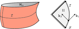
Figure 9: When ${A<\sqrt{-\Lambda/3}}$, the $C$-metric represents a single, uniformly accelerated black hole. The region near infinity ${\mathcal{I}}$ is everywhere static. The first PND ${{\boldsymbol{\mathbf{k}}}}_{1}$ is oriented outside the universe, whereas the second one ${{\boldsymbol{\mathbf{k}}}}_{2}$ points inside it.

We now discuss the case when the acceleration parameter $A$ is small, ${A<\sqrt{-\Lambda/3}}$. As explained in Sec. II.1, the $C$-metric then describes a single uniformly accelerated black hole in an anti–de Sitter universe. Its global structure for a constant $\varphi$ is visualized in Fig. 1. There are no Killing horizons extending to ${\mathcal{I}}$ (which would correspond to ${F_{\scriptscriptstyle{\infty}}=0}$, i.e., ${R_{2}=1}$) since using (47), (10), and ${0\leq G\leq 1}$ there is

$$R_{2}>P_{\scriptscriptstyle{\infty}}=\frac{1}{\sqrt{G_{\scriptscriptstyle{\infty}}}}\geq 1{\mbox{\;,}}$$ (68)

for all $x\in[x_{\mathrm{f}},x_{\mathrm{b}}]$. Accordingly, the region near infinity ${\mathcal{I}}$ is everywhere static. We thus find that the first PND ${{\boldsymbol{\mathbf{k}}}}_{1}$ is always oriented outside, whereas the second one ${{\boldsymbol{\mathbf{k}}}}_{2}$ is always oriented inside the universe, see (65) and Fig. 9.

The corresponding radiation pattern is shown in Fig. 8(a). There exists just one direction along which the outgoing radiation (${\epsilon=+1}$, ${\left\lvert R\right\rvert<1}$) vanishes, namely the direction $R_{\mathrm{m}}=1/R_{2}$. It is the mirrored reflection of the ingoing PND ${{\boldsymbol{\mathbf{k}}}}_{2}$ (see the left part of Fig. 8(a)). In terms of pseudo-spherical parameters the direction is described by Eq. (63), i.e., ${\psi_{\mathrm{m}}=\psi_{2}}$ and ${\phi_{\mathrm{m}}=\phi_{2}=0}$, where $\psi_{2}$ — the boost parameter characterizing ${{\boldsymbol{\mathbf{k}}}}_{2}$ — is given by Eq. (66). The radiation pattern for ingoing radiation (${\epsilon=-1}$, ${\left\lvert R\right\rvert>1}$) is visualized in the right part of Fig. 8(a). Again, there exists just one direction of vanishing radiation given by ${R_{\mathrm{m}}=1/R_{1}=\infty}$ (i.e., ${\psi_{\mathrm{m}}=\psi_{1}=0}$, cf. Eq. (64)), which is also the mirrored reflection of a PND, this time of the outgoing ${{\boldsymbol{\mathbf{k}}}}_{1}$.

V.2 A pair of accelerated black holes

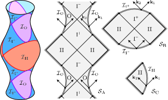
Figure 10: For large values of ${A>\sqrt{-\Lambda/3}}$, the $C$-metric represents pairs of accelerated black holes. The conformal infinity ${\mathcal{I}}$ shown on the left is divided by horizons ${\mathcal{H}}_{\mathrm{c}}$ and ${\mathcal{H}}_{\mathrm{a}}$ into several distinct domains: ${\mathcal{I}}_{\,\mathrm{O}}$ and ${\mathcal{I}}_{\,\mathrm{II}}$ are static, whereas ${\mathcal{I}}_{\,{\mathrm{I}^{+}}}$ and ${\mathcal{I}}_{\,{\mathrm{I}^{-}}}$ are nonstatic. Moreover, in the regions ${\mathcal{I}}_{\,\mathrm{O}}$ (corresponding to sections ${\mathcal{S}_{A}}$) and ${\mathcal{I}}_{\,\mathrm{II}}$ (corresponding to ${\mathcal{S}_{C}}$) the PND ${{\boldsymbol{\mathbf{k}}}}_{1}$ is oriented outwards, whereas the PND ${{\boldsymbol{\mathbf{k}}}}_{2}$ is oriented inwards. In ${\mathcal{I}}_{\,{\mathrm{I}^{+}}}$ (sections ${\mathcal{S}_{B}}$) both ${{\boldsymbol{\mathbf{k}}}}_{1}$ and ${{\boldsymbol{\mathbf{k}}}}_{2}$ point outside the universe, in ${\mathcal{I}}_{\,{\mathrm{I}^{-}}}$ both the PNDs point inside it.

A more interesting but also more complicated situation occurs when ${A>\sqrt{-\Lambda/3}}$. In this case the $C$-metric represents pairs of uniformly accelerated black holes in an anti–de Sitter universe, as indicated in Figs. 2–6, see Sec. II.2. There are (outer) black-hole horizons ${\mathcal{H}}_{\mathrm{o}}$, acceleration horizons ${\mathcal{H}}_{\mathrm{a}}$, and cosmological horizons ${\mathcal{H}}_{\mathrm{c}}$, see Fig. 2(a). At ${\mathcal{I}}$, the horizons ${\mathcal{H}}_{\mathrm{a}}$ and ${\mathcal{H}}_{\mathrm{c}}$ can be identified by ${R_{2}=1}$. They separate various static and nonstatic regions of ${\mathcal{I}}$, and simultaneously the domains of infinity with different structure of the PNDs, as shown in Fig. 10. The vector ${{\boldsymbol{\mathbf{k}}}}_{1}$ is always oriented outside the universe. In the static domains of ${\mathcal{I}}$ where ${R_{2}>1}$, denoted as ${\mathcal{I}}_{\,\mathrm{O}}$ and ${\mathcal{I}}_{\,\mathrm{II}}$, ${{\boldsymbol{\mathbf{k}}}}_{2}$ is oriented inside it; see (65). These domains of the infinity can be reached through the sections ${\mathcal{S}_{A}}$ and ${\mathcal{S}_{C}}$, cf. Figs. 4, 6. On the other hand, in the domain where ${R_{2}<1}$, denoted as ${\mathcal{I}}_{\,{\mathrm{I}^{+}}}$ (accessible through ${\mathcal{S}_{B}}$, Fig. 5), both PNDs are oriented outside the spacetime.

In each of these regions the radiation pattern (56) is thus different. In particular, it admits a different number of directions along which the radiation vanishes. Recalling that the radiation vanishes along mirrored reflections of PNDs, we see that in the static regions ${\mathcal{I}}_{\,\mathrm{O}}$ and ${\mathcal{I}}_{\,\mathrm{II}}$ there is just one outgoing (${\epsilon=+1}$) direction along which the radiation vanishes, as in the previous case of a single black hole. This is the mirrored reflection of ${{\boldsymbol{\mathbf{k}}}}_{2}$, ${R_{\mathrm{m}}=1/R_{2}}$ (${\psi_{\mathrm{m}}=\psi_{2}}$, ${\phi_{\mathrm{m}}=\phi_{2}=0}$, cf. Eq. (63)). The corresponding directional pattern is again given by the left part of Fig. 8(a). However, in the nonstatic region ${\mathcal{I}}_{\,{\mathrm{I}^{+}}}$ there is no outgoing direction along which the radiation vanishes because mirrored reflections of both PNDs are ingoing. In other words, the condition (63) cannot be satisfied because ${R_{2}<1}$. The radiation pattern for outgoing directions for this case is shown in the left part of Fig. 8(b).

Of course, the number of null directions with vanishing radiation in the pattern for ingoing geodesics (${\epsilon=-1}$) is complementary. In the domains ${\mathcal{I}}_{\,\mathrm{O}}$ and ${\mathcal{I}}_{\,\mathrm{II}}$ with ${R_{2}>1}$ there is again just one zero, now given by the mirrored reflection of ${{\boldsymbol{\mathbf{k}}}}_{1}$ (${R_{\mathrm{m}}=\infty}$, ${\psi_{\mathrm{m}}=\psi_{1}=0}$); see the right part of Fig. 8(a). On the other hand, in the domain ${\mathcal{I}}_{\,{\mathrm{I}^{+}}}$ there are exactly two zeros for ingoing radiation given by mirrored reflections of both PNDs (${R_{\mathrm{m}}=\infty}$, ${\psi_{\mathrm{m}}=0}$, and ${R_{\mathrm{m}}=1/R_{2}}$, ${\psi_{\mathrm{m}}=\psi_{2}}$, ${\phi_{\mathrm{m}}=0}$, cf. Eq. (64)) as shown in the right part of Fig. 8(b).

In addition, there is also another domain with $R_{2}<1$, namely the domain ${\mathcal{I}}_{\,{\mathrm{I}^{-}}}$; see Fig. 10. Here both PNDs are oriented inside the spacetime. However, the region ${\mathrm{I}^{-}}$ of the spacetime and its infinity ${\mathcal{I}}_{\,{\mathrm{I}^{-}}}$ are not covered by the same map of Robinson-Trautman coordinates as that used above. We have to introduce another “time-reversed” map to cover the white domain in Fig. 5. Still, the directions of vanishing radiation are given by mirrored directions of the PNDs at the infinity, similarly to the cases discussed above. The mirrored directions of the PNDs are both outgoing so that the radiation pattern for outgoing geodesics contains two zeros (cf. the right part of Fig. 8(b)), whereas the pattern for ingoing geodesics does not have any zero directions, cf. the left part of Fig. 8(b).

To summarize, the directional patterns of outgoing radiation (Eqs. (56) with ${\epsilon=+1}$, or Eqs. (46) with ${\left\lvert R\right\rvert<1}$) in the domains ${\mathcal{I}}_{\,\mathrm{O}}$, ${\mathcal{I}}_{\,{\mathrm{I}^{+}}}$, ${\mathcal{I}}_{\,{\mathrm{I}^{-}}}$, and ${\mathcal{I}}_{\,\mathrm{II}}$ of the conformal infinity are given by the left (a), left (b), right (b), and left (a) parts of Fig. 8, respectively. For ingoing radiation (Eqs. (56) with ${\epsilon=-1}$, or Eqs. (46) with ${\left\lvert R\right\rvert>1}$) these are given by the right (a), right (b), left (b), and right (a) parts of Fig. 8, respectively.

V.3 Vanishing acceleration

Finally, we briefly describe the character of radiation when the acceleration vanishes, in which case the spacetime describes a single nonaccelerating black hole in an anti–de Sitter universe (“Reissner-Nordström-anti–de Sitter solution”). It is thus spherically symmetric with surfaces ${t,y=\text{constant}}$ being the orbits of the rotational group, and radial directions being contained in sections ${x,\varphi=\text{constant}}$. From ${A=0}$ it follows ${R_{2}=\infty}$, cf. Eq. (47), and the above general expressions simplify. In particular for ${A=0}$ not only ${{\boldsymbol{\mathbf{k}}}}_{\scriptscriptstyle\mathrm{RT}}\propto{{\boldsymbol{\mathbf{k}}}}_{1}\propto{\frac{1}{\sqrt{2}}}({{\boldsymbol{\mathbf{t}}}}_{\mathrm{o}}+{{\boldsymbol{\mathbf{q}}}}_{\mathrm{o}})$, but also ${{\boldsymbol{\mathbf{l}}}}_{\scriptscriptstyle\mathrm{RT}}\propto{{\boldsymbol{\mathbf{k}}}}_{2}\propto{\frac{1}{\sqrt{2}}}({{\boldsymbol{\mathbf{t}}}}_{\mathrm{o}}-{{\boldsymbol{\mathbf{q}}}}_{\mathrm{o}})$ is a PND, see Eq. (65); this is consistent with relations (35) in which only the components $\Psi^{{\scriptscriptstyle\mathrm{RT}}}_{2}$ and $\Phi^{{\scriptscriptstyle\mathrm{RT}}}_{1}$ remain nonvanishing. At the infinity ${\mathcal{I}}$ the PNDs are mutually mirrored reflections, ${{\boldsymbol{\mathbf{k}}}}_{1}$ oriented outside the universe and ${{\boldsymbol{\mathbf{k}}}}_{2}$ inside it, parametrized by ${\psi_{1}=0=\psi_{2}}$, see Eqs. (65), (52). Both the PNDs point in radial directions of the spherical symmetry. Moreover, since ${R_{2}>1}$, it follows from relation (67) that the region near ${\mathcal{I}}$ is always static, without the Killing horizon extending there.

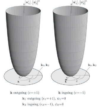
Figure 11: The directional patterns of outgoing/ingoing radiation are the same and axially symmetric when $A=0$. In such a case the PNDs ${{\boldsymbol{\mathbf{k}}}}_{1}$ and ${{\boldsymbol{\mathbf{k}}}}_{2}$ are mutual mirror images under reflection with respect to ${\mathcal{I}}$. Therefore, there is exactly one direction given by $\psi=0$ along which the radiation vanishes, both for outgoing and ingoing null geodesics.

For vanishing acceleration the expressions (56) and (61) reduce to

$$\left\lvert\Psi^{{\mathrm{i}}}_{4}\right\rvert \approx\frac{\left\lvert\Lambda\right\rvert}{4}\frac{m}{\gamma\,\eta}\,\sinh^{2}\psi=\frac{\left\lvert\Lambda\right\rvert}{4}\frac{m}{\gamma\,\eta}\,\tan^{2}\theta{\mbox{\;,}}$$ (69)

$$\left\lvert\Phi^{{\mathrm{i}}}_{2}\right\rvert \approx\sqrt{\frac{\left\lvert\Lambda\right\rvert}{24}}\,\frac{\left\lvert e\right\rvert}{\gamma\,\eta}\,\sinh\psi=\sqrt{\frac{\left\lvert\Lambda\right\rvert}{24}}\,\frac{\left\lvert e\right\rvert}{\gamma\,\eta}\,\left\lvert\tan\theta\right\rvert{\mbox{\;.}}$$

The corresponding directional pattern of radiation, shown in Fig. 11, is axially symmetric and independent of $\epsilon$, i.e., it is the same both for ingoing and outgoing null geodesics. Interestingly, even for a nonaccelerated black hole there is thus radiation on ${\mathcal{I}}$ along any nonradial null direction, i.e., except for ${\psi=0}$, ${\epsilon=\pm 1}$, which corresponds to both PNDs. This may seem quite surprising since the region near infinity is static. It is a completely new specific feature: for ${\Lambda>0}$ a generic, nonradial observer near ${\mathcal{I}}^{+}$ would also detect radiation generated by nonaccelerated black holes Krtouš and Podolský (2003), but the region near infinity is nonstatic. In asymptotically flat spacetimes (${\Lambda=0}$) there is no radiation on ${\mathcal{I}}^{+}$ from black holes with ${A=0}$ Kinnersley and Walker (1970), which, remarkably, also follows from expression (40).

VI Summary

It was observed already in the 1960s by Penrose Penrose (1964, 1965, 1967) that radiation is defined “less invariantly” in spacetimes with a non-null ${\mathcal{I}}$. Recently we have analyzed the $C$-metric solution with ${\Lambda>0}$ Krtouš and Podolský (2003) and found an explicit directional pattern of radiation. This fully characterizes the radiation from uniformly accelerated black holes near the de Sitter-like conformal infinity ${\mathcal{I}}^{+}$, which has a spacelike character. Here we have completed the picture by investigating the radiative properties of the $C$-metric with a negative cosmological constant. This exact solution of the Einstein-Maxwell equations with ${\Lambda<0}$ represents a spacetime in which the radiation is generated either by a (possibly charged) single black hole or pairs of black holes uniformly accelerated in an anti–de Sitter universe.

We have analyzed the asymptotic behavior of the gravitational and electromagnetic fields near the conformal infinity ${\mathcal{I}}$, which has a timelike character. The leading components of the fields have been expressed in a suitable parallelly transported interpretation tetrad. These components are inversely proportional to the affine parameter of the corresponding null geodesic. In addition, an explicit formula (56) [or, equivalently, Eqs. (46) and (61)] which describes the directional pattern of radiation has been derived: it expresses the dependence of the field magnitudes on spacetime directions from which a given point $N_{\scriptscriptstyle{\infty}}$ at infinity ${\mathcal{I}}$ is approached. This specific directional characteristic supplements the peeling property, completing thus the asymptotic behavior of gravitational and electromagnetic fields near infinity ${\mathcal{I}}$ with a timelike character.

We have demonstrated that the situation is much more complicated in the anti–de Sitter case than in the case ${\Lambda>0}$. The new specific feature is that timelike conformal infinity ${\mathcal{I}}$ is, in general, divided by Killing horizons into several static and nonstatic regions with a different structure of (double degenerate) principal null directions. In these distinct domains of infinity the directional patterns of radiation differ. For example, there are different numbers of geometrically privileged directions (namely one, two, or none) in which the radiation vanishes completely. These exactly correspond to mirrored directions of principal null direction, with respect to ${\mathcal{I}}$. Accordingly, there exists an asymmetry between outgoing and ingoing radiation patterns in all the domains.

As in the ${\Lambda>0}$ case Krtouš et al. (2003), it seems plausible that a general structure of the radiation pattern at conformal infinity depends only on the PNDs there, i.e., it is given by the algebraic (Petrov) type of the spacetime. This hypothesis will be proven elsewhere Krtouš and Podolský .

Appendix A Radiation along some particular null geodesics

Here we concentrate on a geometrically privileged family of special geodesics which asymptotically take the form Eq. (27) with ${c=0}$. It follows from (28) that this corresponds either to outgoing null geodesics with ${d=0}$ or ingoing ones with ${d=-6/\Lambda}$.

In fact, the geodesics ${c=0=d}$ are exact null geodesics

$$u=u_{\scriptscriptstyle{\infty}}=\text{constant}{\mbox{\;,\quad}}\zeta=\zeta_{\scriptscriptstyle{\infty}}=\text{constant}{\mbox{\;,\quad}}$$ (70)

in the whole spacetime, with $r$ being their affine parameter. They approach infinity ${\mathcal{I}}$ along the (double degenerate) principal null direction ${{{\boldsymbol{\mathbf{k}}}}_{\scriptscriptstyle\mathrm{RT}}={{\boldsymbol{\mathbf{\partial}}}_{r}}}$, which is characterized by the parameter ${\psi=0}$, see Eq. (55) (or by ${\theta=0}$). It can be shown that the Robinson-Trautman tetrad (34) is parallelly transported along these geodesics,

$${{\boldsymbol{\mathbf{k}}}}_{\scriptscriptstyle\mathrm{RT}}\cdot\nabla{{\boldsymbol{\mathbf{k}}}}_{\scriptscriptstyle\mathrm{RT}}=0{\mbox{\;,\quad}}{{\boldsymbol{\mathbf{k}}}}_{\scriptscriptstyle\mathrm{RT}}\cdot\nabla{{\boldsymbol{\mathbf{l}}}}_{\scriptscriptstyle\mathrm{RT}}=0{\mbox{\;,\quad}}{{\boldsymbol{\mathbf{k}}}}_{\scriptscriptstyle\mathrm{RT}}\cdot\nabla{{\boldsymbol{\mathbf{m}}}}_{\scriptscriptstyle\mathrm{RT}}=0{\mbox{\;,}}$$ (71)

and it is also invariant under a shift along the Killing vector ${{\boldsymbol{\mathbf{\partial}}}_{t}}$, i.e., ${\mathcal{L}_{{{\boldsymbol{\mathbf{\partial}}}_{t}}}{{\boldsymbol{\mathbf{k}}}}_{\scriptscriptstyle\mathrm{RT}}=0}$, ${\mathcal{L}_{{{\boldsymbol{\mathbf{\partial}}}_{t}}}{{\boldsymbol{\mathbf{l}}}}_{\scriptscriptstyle\mathrm{RT}}=0}$, ${\mathcal{L}_{{{\boldsymbol{\mathbf{\partial}}}_{t}}}{{\boldsymbol{\mathbf{m}}}}_{\scriptscriptstyle\mathrm{RT}}=0}$, respecting thus a symmetry of the spacetime. Consequently, we can naturally set the interpretation tetrad ${({{\boldsymbol{\mathbf{k}}}}_{\mathrm{i}},\,{{\boldsymbol{\mathbf{l}}}}_{\mathrm{i}},\,{{\boldsymbol{\mathbf{m}}}}_{\mathrm{i}},\,{\bar{{\boldsymbol{\mathbf{m}}}}}_{\mathrm{i}})}\equiv{({{\boldsymbol{\mathbf{k}}}}_{\scriptscriptstyle\mathrm{RT}},\,{{\boldsymbol{\mathbf{l}}}}_{\scriptscriptstyle\mathrm{RT}},\,{{\boldsymbol{\mathbf{m}}}}_{\scriptscriptstyle\mathrm{RT}},\,{\bar{{\boldsymbol{\mathbf{m}}}}}_{\scriptscriptstyle\mathrm{RT}})}$ in the whole spacetime, not only asymptotically near ${\mathcal{I}}$, as in (37) for ${c=0}$, ${d=0}$. As follows from Eqs. (35), all components of gravitational and electromagnetic fields are explicitly given by

$$\Psi^{{\mathrm{i}}}_{4} =-\frac{3A^{2}}{P}\,\Bigl{(}m+2\,e^{2}A\,x-\frac{e^{2}}{r}\Bigr{)}\,\,\frac{1}{r}{\mbox{\;,}}$$ (72)

$$\Psi^{{\mathrm{i}}}_{3} =\frac{3A}{\sqrt{2}\,P}\,\Bigl{(}m+2\,e^{2}A\,x-\frac{e^{2}}{r}\Bigr{)}\,\frac{1}{r^{2}}{\mbox{\;,}}$$

$$\Psi^{{\mathrm{i}}}_{2} =-\Bigl{(}m+2\,e^{2}A\,x-\frac{e^{2}}{r}\Bigr{)}\,\frac{1}{r^{3}}{\mbox{\;,\quad}}\Psi^{{\mathrm{i}}}_{1}=\Psi^{{\mathrm{i}}}_{0}=0{\mbox{\;,}}$$

and

$$\Phi^{{\mathrm{i}}}_{2}=\frac{e\,A}{\sqrt{2}\,P}\,\frac{1}{r}{\mbox{\;,\quad}}\Phi^{{\mathrm{i}}}_{1}=-\frac{e}{2}\,\frac{1}{r^{2}}{\mbox{\;,\quad}}\Phi^{{\mathrm{i}}}_{0}=0{\mbox{\;.}}$$ (73)

Clearly, the leading terms in the ${1/r}$ expansion give the previous general asymptotical results (40) with ${c=0=d}$. In the case of anti–de Sitter spacetime (${m=0}$, ${e=0}$) the field components obviously identically vanish. In the general case the fields have a radiative character (${\sim 1/r}$) except for a vanishing acceleration $A$ and/or for ${P=\infty}$. The interesting “static” limiting case ${A=0}$ has been already discussed in Sec. V.3. The case ${P=\infty}$ corresponds to observers located at the privileged position where ${G=0}$, i.e., on the axes ${x=x_{\mathrm{b}}}$ and ${x=x_{\mathrm{f}}}$ where the strings/struts are localized. This is analogous to the situation when $\Lambda>0$ Krtouš and Podolský (2003), and an electromagnetic field of accelerated test charges in flat spacetime: this is also not radiative along the axis of symmetry, which is the direction of acceleration.

Let us also recall (see Krtouš and Podolský (2003)) that the affine parameter $r$ coincides both with the luminosity and the parallax distance for the congruence of the above null geodesics. The radiative ${1/r}$ fall-off of the fields is naturally measurable (even locally) by observers moving radially to infinity, using both the luminosity and the parallax methods for determining the distance.

Concerning the other special family of ingoing null geodesics, ${c=0}$, ${d=-6/\Lambda}$, $\epsilon=-1$, it can be observed that the transformation given by (36) becomes singular and (37) is not thus justified. However, from Eqs. (24), (33), and (34), with the condition (38) for fixing ${{\boldsymbol{\mathbf{l}}}}_{\mathrm{i}}$, it follows that in this case

$${{\boldsymbol{\mathbf{k}}}}_{\mathrm{i}} \approx-\frac{1}{\gamma^{2}\,\eta^{2}}\biggl{(}r^{2}\,{{\boldsymbol{\mathbf{\partial}}}_{r}}+\frac{6}{\Lambda}\,{{\boldsymbol{\mathbf{\partial}}}_{u}}\,\biggr{)}\approx-\frac{6}{\Lambda}\frac{1}{\gamma^{2}\eta^{2}}\,{{\boldsymbol{\mathbf{l}}}}_{\scriptscriptstyle\mathrm{RT}}{\mbox{\;,}}$$ (74)

$${{\boldsymbol{\mathbf{l}}}}_{\mathrm{i}} \approx-\frac{\Lambda}{6}r^{2}\,{{\boldsymbol{\mathbf{\partial}}}_{r}}\approx-\frac{\Lambda}{6}\gamma^{2}\eta^{2}\,{{\boldsymbol{\mathbf{k}}}}_{\scriptscriptstyle\mathrm{RT}}{\mbox{\;,}}$$

which — somewhat surprisingly — fully agrees with expressions (37) for the special case ${c=0}$, ${d=-6/\Lambda}$. Thus the interpretation tetrad along these geodesics is equivalent to the tetrad (37) along the PND given by ${c=0}$, ${d=0}$ (which itself agrees with the Robinson-Trautman tetrad (34)) after interchanging ${{{\boldsymbol{\mathbf{k}}}}_{\mathrm{i}}\leftrightarrow{{\boldsymbol{\mathbf{l}}}}_{\mathrm{i}}}$ and ${{{\boldsymbol{\mathbf{m}}}}_{\mathrm{i}}\leftrightarrow-{\bar{{\boldsymbol{\mathbf{m}}}}}_{\mathrm{i}}}$, accompanied by a boost (83) with ${B=-6/(\Lambda r^{2})}$. Components of the gravitational and electromagnetic fields can thus easily be obtained from (72), (73). In particular, it follows that ${\Psi^{{\mathrm{i}}}_{4}\approx 0\approx\Psi^{{\mathrm{i}}}_{3}}$, ${\Psi^{{\mathrm{i}}}_{2}\sim\eta^{-3}}$, ${\Psi^{{\mathrm{i}}}_{1}\sim\eta^{-4}}$, ${\Psi^{{\mathrm{i}}}_{0}\sim\eta^{-5}}$, and ${\Phi^{{\mathrm{i}}}_{2}\approx 0}$, ${\Phi^{{\mathrm{i}}}_{1}\sim\eta^{-2}}$, ${\Phi^{{\mathrm{i}}}_{0}\sim\eta^{-3}}$. Obviously, the radiative parts of the fields vanish along these special ingoing geodesics, which agrees with the expression ${\psi_{\mathrm{m}}=0}$ in (64), cf. (55). Indeed, this direction is just the reflection of the PND ${{\boldsymbol{\mathbf{k}}}}_{1}$.

Appendix B Transformations of the components $\Psi_{n}$ and $\Phi_{n}$

The Weyl tensor can be parametrized by five standard complex coefficients defined as components with respect to a null tetrad (see, e.g., Kramer et al. (1980)):

$$\Psi_{0} ={\mspace{14.5mu}}{\boldsymbol{\mathbf{C}}}_{\alpha\beta\gamma\delta}\,{{\boldsymbol{\mathbf{k}}}}^{\alpha}\,{{\boldsymbol{\mathbf{m}}}}^{\beta}\,{{\boldsymbol{\mathbf{k}}}}^{\gamma}\,{{\boldsymbol{\mathbf{m}}}}^{\delta}{\mbox{\;,}}$$ (75)

$$\Psi_{1} ={\mspace{14.5mu}}{\boldsymbol{\mathbf{C}}}_{\alpha\beta\gamma\delta}\,{{\boldsymbol{\mathbf{k}}}}^{\alpha}\,{{\boldsymbol{\mathbf{l}}}}^{\beta}\,{{\boldsymbol{\mathbf{k}}}}^{\gamma}\,{{\boldsymbol{\mathbf{m}}}}^{\delta}{\mbox{\;,}}$$

$$\Psi_{2} =-{\boldsymbol{\mathbf{C}}}_{\alpha\beta\gamma\delta}\,{{\boldsymbol{\mathbf{k}}}}^{\alpha}\,{{\boldsymbol{\mathbf{m}}}}^{\beta}\,{{\boldsymbol{\mathbf{l}}}}^{\gamma}\,{\bar{{\boldsymbol{\mathbf{m}}}}}^{\delta}{\mbox{\;,}}$$

$$\Psi_{3} ={\mspace{14.5mu}}{\boldsymbol{\mathbf{C}}}_{\alpha\beta\gamma\delta}\,{{\boldsymbol{\mathbf{l}}}}^{\alpha}\,{{\boldsymbol{\mathbf{k}}}}^{\beta}\,{{\boldsymbol{\mathbf{l}}}}^{\gamma}\,{\bar{{\boldsymbol{\mathbf{m}}}}}^{\delta}{\mbox{\;,}}$$

$$\Psi_{4} ={\mspace{14.5mu}}{\boldsymbol{\mathbf{C}}}_{\alpha\beta\gamma\delta}\,{{\boldsymbol{\mathbf{l}}}}^{\alpha}\,{\bar{{\boldsymbol{\mathbf{m}}}}}^{\beta}\,{{\boldsymbol{\mathbf{l}}}}^{\gamma}\,{\bar{{\boldsymbol{\mathbf{m}}}}}^{\delta}{\mbox{\;.}}$$

Similarly, the tensor of electromagnetic field is parametrized as

$$\Phi_{0} ={\boldsymbol{\mathbf{F}}}_{\alpha\beta}\,{{\boldsymbol{\mathbf{k}}}}^{\alpha}\,{{\boldsymbol{\mathbf{m}}}}^{\beta}{\mbox{\;,}}$$ (76)

$$\Phi_{1} ={\textstyle\frac{1}{2}}\,{\boldsymbol{\mathbf{F}}}_{\alpha\beta}\,\bigl{(}{{\boldsymbol{\mathbf{k}}}}^{\alpha}\,{{\boldsymbol{\mathbf{l}}}}^{\beta}-{{\boldsymbol{\mathbf{m}}}}^{\alpha}\,{\bar{{\boldsymbol{\mathbf{m}}}}}^{\beta}\bigr{)}{\mbox{\;,}}$$

$$\Phi_{2} ={\boldsymbol{\mathbf{F}}}_{\alpha\beta}\,{\bar{{\boldsymbol{\mathbf{m}}}}}^{\alpha}\,{{\boldsymbol{\mathbf{l}}}}^{\beta}{\mbox{\;.}}$$

These transform in a well-known way under the following particular Lorentz transformations. For a null rotation with ${{\boldsymbol{\mathbf{k}}}}$ fixed, $L\in\mathbb{C}$,

$$\begin{aligned} {{\boldsymbol{\mathbf{k}}}}&={{\boldsymbol{\mathbf{k}}}}_{\mathrm{o}}{\mbox{\;,}}\\ {{\boldsymbol{\mathbf{l}}}}&={{\boldsymbol{\mathbf{l}}}}_{\mathrm{o}}+\bar{L}{{\boldsymbol{\mathbf{m}}}}_{\mathrm{o}}+L{\bar{{\boldsymbol{\mathbf{m}}}}}_{\mathrm{o}}+L\bar{L}{{\boldsymbol{\mathbf{k}}}}_{\mathrm{o}}{\mbox{\;,}}\\ {{\boldsymbol{\mathbf{m}}}}&={{\boldsymbol{\mathbf{m}}}}_{\mathrm{o}}+L{{\boldsymbol{\mathbf{k}}}}_{\mathrm{o}}{\mbox{\;,}}\end{aligned}$$ (77)

$$\begin{aligned} \Psi_{0}&=\Psi^{{\mathrm{o}}}_{0}{\mbox{\;,}}\\ \Psi_{1}&={\bar{L}}\,\Psi^{{\mathrm{o}}}_{0}+\Psi^{{\mathrm{o}}}_{1}{\mbox{\;,}}\\ \Psi_{2}&={\bar{L}}^{2}\Psi^{{\mathrm{o}}}_{0}+2{\bar{L}}\,\Psi^{{\mathrm{o}}}_{1}+\Psi^{{\mathrm{o}}}_{2}{\mbox{\;,}}\\ \Psi_{3}&={\bar{L}}^{3}\Psi^{{\mathrm{o}}}_{0}+3{\bar{L}}^{2}\Psi^{{\mathrm{o}}}_{1}+3{\bar{L}}\,\Psi^{{\mathrm{o}}}_{2}+\Psi^{{\mathrm{o}}}_{3}{\mbox{\;,}}\\ \Psi_{4}&={\bar{L}}^{4}\Psi^{{\mathrm{o}}}_{0}+4{\bar{L}}^{3}\Psi^{{\mathrm{o}}}_{1}+6{\bar{L}}^{2}\Psi^{{\mathrm{o}}}_{2}+4{\bar{L}}\,\Psi^{{\mathrm{o}}}_{3}+\Psi^{{\mathrm{o}}}_{4}{\mbox{\;,}}\end{aligned}$$ (78)

$$\begin{aligned} \Phi_{0}&=\Phi^{{\mathrm{o}}}_{0}{\mbox{\;,}}\\ \Phi_{1}&={\bar{L}}\,\Phi^{{\mathrm{o}}}_{0}+\Phi^{{\mathrm{o}}}_{1}{\mbox{\;,}}\\ \Phi_{2}&={\bar{L}}^{2}\Phi^{{\mathrm{o}}}_{0}+2{\bar{L}}\,\Phi^{{\mathrm{o}}}_{1}+\Phi^{{\mathrm{o}}}_{2}{\mbox{\;.}}\end{aligned}$$ (79)

Under a null rotation with ${{\boldsymbol{\mathbf{l}}}}$ fixed, $K\in\mathbb{C}$,

$$\begin{aligned} {{\boldsymbol{\mathbf{k}}}}&={{\boldsymbol{\mathbf{k}}}}_{\mathrm{o}}+\bar{K}{{\boldsymbol{\mathbf{m}}}}_{\mathrm{o}}+K{\bar{{\boldsymbol{\mathbf{m}}}}}_{\mathrm{o}}+K\bar{K}{{\boldsymbol{\mathbf{l}}}}_{\mathrm{o}}{\mbox{\;,}}\\ {{\boldsymbol{\mathbf{l}}}}&={{\boldsymbol{\mathbf{l}}}}_{\mathrm{o}}{\mbox{\;,}}\\ {{\boldsymbol{\mathbf{m}}}}&={{\boldsymbol{\mathbf{m}}}}_{\mathrm{o}}+K{{\boldsymbol{\mathbf{l}}}}_{\mathrm{o}}{\mbox{\;,}}\end{aligned}$$ (80)

$$\begin{aligned} \Psi_{0}&=K^{4}\Psi^{{\mathrm{o}}}_{4}+4K^{3}\Psi^{{\mathrm{o}}}_{3}+6K^{2}\Psi^{{\mathrm{o}}}_{2}+4K\,\Psi^{{\mathrm{o}}}_{1}+\Psi^{{\mathrm{o}}}_{0}{\mbox{\;,}}\\ \Psi_{1}&=K^{3}\Psi^{{\mathrm{o}}}_{4}+3K^{2}\Psi^{{\mathrm{o}}}_{3}+3K\,\Psi^{{\mathrm{o}}}_{2}+\Psi^{{\mathrm{o}}}_{1}{\mbox{\;,}}\\ \Psi_{2}&=K^{2}\Psi^{{\mathrm{o}}}_{4}+2K\,\Psi^{{\mathrm{o}}}_{3}+\Psi^{{\mathrm{o}}}_{2}{\mbox{\;,}}\\ \Psi_{3}&=K\,\Psi^{{\mathrm{o}}}_{4}+\Psi^{{\mathrm{o}}}_{3}{\mbox{\;,}}\\ \Psi_{4}&=\Psi^{{\mathrm{o}}}_{4}{\mbox{\;,}}\end{aligned}$$ (81)

$$\begin{aligned} \Phi_{0}&=K^{2}\Phi^{{\mathrm{o}}}_{2}+2K\,\Phi^{{\mathrm{o}}}_{1}+\Phi^{{\mathrm{o}}}_{0}{\mbox{\;,}}\\ \Phi_{1}&=K\,\Phi^{{\mathrm{o}}}_{2}+\Phi^{{\mathrm{o}}}_{1}{\mbox{\;,}}\\ \Phi_{2}&=\Phi^{{\mathrm{o}}}_{2}{\mbox{\;.}}\end{aligned}$$ (82)

Under a boost in the ${{{\boldsymbol{\mathbf{k}}}}{\text{-}}{{\boldsymbol{\mathbf{l}}}}}$ plane and a spatial rotation in the ${{{\boldsymbol{\mathbf{m}}}}{\text{-}}{\bar{{\boldsymbol{\mathbf{m}}}}}}$ plane given by

$$\begin{gathered}{{\boldsymbol{\mathbf{k}}}}=B\,{{\boldsymbol{\mathbf{k}}}}_{\mathrm{o}}{\mbox{\;,\quad}}{{\boldsymbol{\mathbf{l}}}}=B^{-1}\,{{\boldsymbol{\mathbf{l}}}}_{\mathrm{o}}{\mbox{\;,}}\\ {{\boldsymbol{\mathbf{m}}}}=\exp(i\Phi)\,{{\boldsymbol{\mathbf{m}}}}_{\mathrm{o}}{\mbox{\;,\quad}}\end{gathered}$$ (83)

$B,\Phi\in\mathbb{R}$, the components $\Psi_{n}$ and $\Phi_{n}$ transform as

$$\begin{aligned} \Psi_{0}&=B^{2}\,\exp(2i\Phi)\;\Psi^{{\mathrm{o}}}_{0}{\mbox{\;,}}\\ \Psi_{1}&=B\;\;\exp(i\Phi)\;\Psi^{{\mathrm{o}}}_{1}{\mbox{\;,}}\\ \Psi_{2}&=\Psi^{{\mathrm{o}}}_{2}{\mbox{\;,}}\\ \Psi_{3}&=B^{-1}\;\exp(-i\Phi)\;\Psi^{{\mathrm{o}}}_{3}{\mbox{\;,}}\\ \Psi_{4}&=B^{-2}\,\exp(-2i\Phi)\;\Psi^{{\mathrm{o}}}_{4}{\mbox{\;,}}\end{aligned}$$ (84)

$$\begin{aligned} \Phi_{0}&=B\;\;\exp(i\Phi)\;\Phi^{{\mathrm{o}}}_{0}{\mbox{\;,}}\\ \Phi_{1}&=\Phi^{{\mathrm{o}}}_{1}{\mbox{\;,}}\\ \Phi_{2}&=B^{-1}\,\exp(-i\Phi)\;\Phi^{{\mathrm{o}}}_{2}{\mbox{\;.}}\end{aligned}$$ (85)

References

- Bondi et al. (1962) H. Bondi, M. G. J. van der Burg, and A. W. K. Metzner, Proc. R. Soc. Lond., Ser A 269, 21 (1962).
- Sachs (1962) R. K. Sachs, Proc. R. Soc. Lond., Ser A 270, 103 (1962).
- Newman and Penrose (1962) E. T. Newman and R. Penrose, J. Math. Phys. 3, 566 (1962).
- Newman and Unti (1962) E. T. Newman and T. W. J. Unti, J. Math. Phys. 3, 891 (1962).
- van der Burg (1969) M. G. J. van der Burg, Proc. R. Soc. Lond., Ser A 310, 221 (1969).
- Bičák and Pravdová (1998) J. Bičák and A. Pravdová, J. Math. Phys. 39, 6011 (1998), eprint gr-qc/9808068.
- Pirani (1965) F. A. E. Pirani, in Brandeis Lectures on General Relativity, edited by S. Deser and K. W. Ford (Prentice-Hall, Englewood Cliffs, NJ, 1965), pp. 249–372.
- Bičák (1985) J. Bičák, in Galaxies, Axisymmetric Systems and Relativity, edited by M. A. H. MacCaluum (Cambridge University Press, Cambridge, England, 1985), pp. 91–124.
- Bičák (1997) J. Bičák, in Relativistic Gravitation and Gravitational Radiation, Les Houches 1995, edited by J.-A. Marck and J.-P. Lasota (Cambridge University Press, Cambridge, 1997), pp. 67–87.
- Bičák (2000) J. Bičák, in Einstein’s Field Equations and Their Physical Implications, edited by B. G. Schmidt (Springer, Berlin, 2000), vol. 540, pp. 1–126, eprint gr-qc/0004016.
- Penrose (1963) R. Penrose, Phys. Rev. Lett. 10, 66 (1963).
- Penrose (1964) R. Penrose, in Relativity, Groups and Topology, Les Houches 1963, edited by C. DeWitt and B. DeWitt (Gordon and Breach, New York, 1964), pp. 563–584.
- Penrose (1965) R. Penrose, Proc. R. Soc. Lond., Ser A 284, 159 (1965).
- Penrose and Rindler (1986) R. Penrose and W. Rindler, Spinors and Space-Time, vol. 2 (Cambridge University Press, Cambridge, England, 1986).
- Tafel and Pukas (2000) J. Tafel and S. Pukas, Class. Quantum Grav. 17, 1559 (2000).
- Ashtekar and Magnon (1984) A. Ashtekar and A. Magnon, Class. Quantum Grav. 1, L39 (1984).
- Ashtekar and Das (2000) A. Ashtekar and S. Das, Class. Quantum Grav. 17, L17 (2000), eprint hep-th/9911230.
- Penrose (1967) R. Penrose, in The Nature of Time, edited by T. Gold (Cornell University Press, Ithaca, NY, 1967), pp. 42–54.
- Bičák and Krtouš (2002) J. Bičák and P. Krtouš, Phys. Rev. Lett. 88, 211101 (2002), eprint gr-qc/0207010.
- Krtouš and Podolský (2003) P. Krtouš and J. Podolský, Phys. Rev. D 68, 024005 (2003), eprint gr-qc/0301110.
- Bičák and Krtouš (2001) J. Bičák and P. Krtouš, Phys. Rev. D 64, 124020 (2001), eprint gr-qc/0107078.
- Avis et al. (1978) S. J. Avis, C. J. Isham, and D. Storey, Phys. Rev. D 18, 3565 (1978).
- Hawking (1983) S. W. Hawking, Phys. Lett. B126, 175 (1983).
- Friedrich (1995) H. Friedrich, J. Geom. Phys. 17, 125 (1995).
- Bičák and Schmidt (1989) J. Bičák and B. G. Schmidt, Phys. Rev. D 40, 1827 (1989).
- Bičák (1968) J. Bičák, Proc. R. Soc. Lond., Ser A 302, 201 (1968).
- Pravda and Pravdová (2000) V. Pravda and A. Pravdová, Czech. J. Phys. 50, 333 (2000), eprint gr-qc/0003067.
- Levi-Civita (1917) T. Levi-Civita, Atti Accad. Naz. Lincei, Cl. Sci. Fis., Mat. Nat., Rend. 26, 307 (1917).
- Weyl (1918) H. Weyl, Ann. Phys. (Leipzig) 59, 185 (1918).
- Ehlers and Kundt (1962) J. Ehlers and W. Kundt, in Gravitation: an Introduction to Current Research, edited by L. Witten (John Wiley, New York, 1962), pp. 49–101.
- Kramer et al. (1980) D. Kramer, H. Stephani, E. Herlt, and M. MacCallum, Exact Solutions of Einstein’s Field Equations (Cambridge University Press, Cambridge, England, 1980).
- Kinnersley and Walker (1970) W. Kinnersley and M. Walker, Phys. Rev. D 2, 1359 (1970).
- Farhoosh and Zimmerman (1979) H. Farhoosh and R. L. Zimmerman, J. Math. Phys. 20, 2272 (1979).
- Ashtekar and Dray (1981) A. Ashtekar and T. Dray, Commun. Math. Phys. 79, 581 (1981).
- Bonnor (1983) W. B. Bonnor, Gen. Rel. Grav. 15, 535 (1983).
- Bičák and Pravda (1999) J. Bičák and V. Pravda, Phys. Rev. D 60, 044004 (1999), eprint gr-qc/9902075.
- Letelier and Oliveira (2001) P. S. Letelier and S. R. Oliveira, Phys. Rev. D 64, 064005 (2001), eprint gr-qc/9809089.
- Dias and Lemos (2003a) O. J. C. Dias and J. P. S. Lemos, Phys. Rev. D 67, 064001 (2003a), eprint hep-th/0210065.
- Plebański and Demiański (1976) J. Plebański and M. Demiański, Ann. Phys. (N.Y.) 98, 98 (1976).
- Carter (1968) B. Carter, Commun. Math. Phys. 10, 280 (1968).
- Debever (1971) R. Debever, Bull. Soc. Math. Belg. 23, 360 (1971).
- (42) O. J. C. Dias and J. P. S. Lemos, Phys. Rev. D 68, 104010 (2003), eprint hep-th/0306194.
- Mann and Ross (1995) R. B. Mann and S. F. Ross, Phys. Rev. D 52, 2254 (1995), eprint gr-qc/9504015.
- Mann (1997) R. B. Mann, Class. Quantum Grav. 14, L109 (1997), eprint gr-qc/9607071.
- Mann (1998) R. B. Mann, Nucl. Phys. B516, 357 (1998), eprint hep-th/9705223.
- Booth and Mann (1999) I. S. Booth and R. B. Mann, Nucl. Phys. B539, 267 (1999), eprint gr-qc/9806056.
- Podolský and Griffiths (2001) J. Podolský and J. B. Griffiths, Phys. Rev. D 63, 024006 (2001), eprint gr-qc/0010109.
- Dias and Lemos (2003b) O. J. C. Dias and J. P. S. Lemos, Phys. Rev. D 67, 084018 (2003b), eprint hep-th/0301046.
- Emparan et al. (2000b) R. Emparan, G. T. Horowitz, and R. C. Myers, J. High Energy Phys. 01, 021 (2000b), eprint hep-th/9912135.
- Podolský (2002) J. Podolský, Czech. J. Phys. 52, 1 (2002), eprint gr-qc/0202033.
- Emparan et al. (2000a) R. Emparan, G. T. Horowitz, and R. C. Myers, JHEP 01, 007 (2000a), eprint hep-th/9911043.
- Chamblin (2001) A. Chamblin, Class. Quantum Grav. 18, L17 (2001), eprint hep-th/0011128.
- Walker and Penrose (1970) M. Walker and R. Penrose, Commun. Math. Phys. 18, 265 (1970).
- Hughston et al. (1972) L. P. Hughston, R. Penrose, P. Sommers, and M. Walker, Commun. Math. Phys. 27, 303 (1972).
- Henneaux and Teitelboim (1985) M. Henneaux and C. Teitelboim, Commun. Math. Phys. 98, 391 (1985).
- (56) P. Krtouš and J. Podolský, Gravitational and electromagnetic fields near anti-de Sitter-like infinity, eprint gr-qc/0310089.
- Krtouš et al. (2003) P. Krtouš, J. Podolský, and J. Bičák, Phys. Rev. Lett. 91, 061101 (2003), eprint gr-qc/0308004.