Quasinormal Modes in three-dimensional time-dependent Anti-de Sitter spacetime

Abstract

The massless scalar wave propagation in the time-dependent BTZ black hole background has been studied. It is shown that in the quasi-normal ringing both the decay and oscillation time-scales are modified in the time-dependent background.

Quasinormal modes of black holes have been an intriguing subject of discussions over thirty years 1 , leading to important contributions to the understanding of black holes 2 ; 3 ; 4 ; 5 . Up until very recently, all works in this field deal with asymptotically flat spacetimes. In the past few years the study has been extended to de Sitter space 6 ; 7 as well as Andi-de-Sitter space 8 ; 9 ; 10 ; 11 . In addition to the astronomical interest that quasinormal modes carry a unique fingerprint which would lead to the direct identification of the black hole existence, quasinormal modes is a good testing ground which gives evidence of the correspondence between gravity in AdS(dS) spacetime and quantum field theory at the boundary.

So far the study of quasinormal modes is restricted to time-independent black hole backgrounds. It should be realized that it is realistic to consider a black hole with parameters changing with time due to the absorption or evaporation processes. Recently the influence of the time-dependent spacetime effect on the late-time tail behavior of the perturbation on the black hole background has been explored 12 . In our previous work 13 , we have investigated the modification to the quasinormal modes in the dynamic Schwarzschild black hole background. The temporal evolution of massless scalar field perturbation, especially the quasinormal modes in different time-dependent situation have been obtained. It is of interest to extend our study to time-dependent AdS spacetime. AdS spacetime share with asymptotically flat spacetimes the common property which makes it a good testing ground what one wants to go beyond asymptotic flatness. Besides exploring the quasinormal modes in time-dependent AdS spacetime can provide further understanding to the AdS/CFT correspondence.

We will concentrate on 3D non-rotating BTZ black hole 14 with the metric

$$ds^{2}=\left(-M+\frac{r^{2}}{l^{2}}\right)dt^{2}-\left(-M+\frac{r^{2}}{l^{2}}\right)^{-1}dr^{2}-r^{2}d\phi^{2}$$ (1)

and $\Lambda=-1/l^{2}$

In this general stationary coordinate, the quasinormal modes and associated frequencies are studied in 11 . However, this coordinate is not appropriate to be used to study the time-dependent case 13 . One option is to use the Kruskal-like coordinate in time-dependent problems. Here we first show that Kruskal coordinate is valid in studying the wave propagation in stationary BTZ black hole.

The Kruskal coordinate for the BTZ black hole is given by 14

$$ds^{2}=\Omega^{2}\left(d\tau^{2}-d\rho^{2}\right)-r^{2}d\phi^{2}$$ (2)

where $\tau$ and $\rho$ are the time-like and space-like coordinates respectively. For $r\geq r_{+}$, they are defined by

$$r_{+}<r\leq\infty\left\{\begin{array}[]{lcl}\rho&=&\sqrt{\frac{r-r_{+}}{r+r_{+}}}\cosh a_{+}t\\[20.0pt] \tau&=&\sqrt{\frac{r-r_{+}}{r+r_{+}}}\sinh a_{+}t\\ \end{array}\right.$$ (3)

where

$$a_{+}=\frac{\sqrt{M}}{l},\;\;\;\;\;r_{+}=l\sqrt{M},\;\;\;\;\;\Omega^{2}(r,t)=\left(\frac{r}{\sqrt{M}}+l\right)^{2}$$

The relation between $\tau$, $\rho$ and $t$, $r$ are

$$t=\frac{l}{2\sqrt{M}}\ln\left(\frac{1+\tau/\rho}{1-\tau/\rho}\right)$$ (4)

$$r=\frac{1+(\rho^{2}-\tau^{2})}{1-(\rho^{2}-\tau^{2})}l\sqrt{M}$$ (5)

The propagation of the massless scalar field in Kruskal coordinates is governed by

$$\frac{1}{\sqrt{r}}\left(\Psi_{,\,\tau\tau}-\Psi_{,\,\rho\rho}\right)+\left(-\frac{r^{\prime 2}-\dot{r}^{2}}{4r^{5/2}}+\frac{r^{\prime\prime}-\ddot{r}}{2r^{3/2}}+\frac{m^{2}}{r^{5/2}}\Omega^{2}\right)\Psi=0$$ (6)

where $m$ is the angular quantum number.

Analogous to the null coordinates used in 4 , we make the variable transformations

$$u=\tau-\rho,\;\;\;\;\;v=\tau+\rho$$ (7)

then the expression of $t$ and $r$ are

$$t=\frac{l}{2\sqrt{M}}\ln\left(-\frac{v}{u}\right)$$ (8)

$$r=\frac{1-uv}{1+uv}l\sqrt{M}$$ (9)

and $r$ will be a function of $u$ and $v$, $r=r(u,v)$, and $\frac{\partial}{\partial\tau}=\frac{\partial}{\partial v}+\frac{\partial}{\partial u}$, $\frac{\partial}{\partial\rho}=\frac{\partial}{\partial v}-\frac{\partial}{\partial u}$.

Equation (6) becomes

$$\frac{4}{\sqrt{r}}\Psi_{,\,uv}+\left(\frac{1}{r^{5/2}}\frac{\partial r}{\partial v}\frac{\partial r}{\partial u}-\frac{2}{r^{3/2}}\frac{\partial^{2}r}{\partial u\partial v}+\frac{m^{2}}{r^{5/2}}\Omega^{2}\right)\Psi=0$$ (10)

Taking

$$u^{*}=\ln\left(-\frac{1}{u}\right)\;\;\;\;\;\;\;\;\;\;\;\;\;\;\;\;\;\;\;\;\;\;\;\;\;\;\;\;\;\;\;\;\;\;\;v^{*}=\ln v$$

we have

$$\left\{\begin{array}[]{lcl}t&=&\frac{l}{\sqrt{M}}\frac{v^{*}+u^{*}}{2}\\[20.0pt] r^{*}&=&\frac{l}{\sqrt{M}}\frac{v^{*}-u^{*}}{2}\\[20.0pt] r&=&-l\sqrt{M}\coth\left(\frac{\sqrt{M}}{l}r_{*}\right)\end{array}\right.$$ (11)

Eq.(10) can be written as

$$-4\Psi_{,\,u^{*}v^{*}}=V\Psi$$ (12)

where the effective potential reads

$$V=\frac{r-r_{+}}{r+r_{+}}\left(\frac{1}{r^{2}}\frac{\partial r}{\partial v}\frac{\partial r}{\partial u}-\frac{2}{r}\frac{\partial^{2}r}{\partial u\partial v}+\frac{m^{2}}{r^{2}}\Omega^{2}\right)$$ (13)

This potential diverges when $r\rightarrow\infty$, which has the same property as that in general coordinates (1). This divergence can be overcome by imposing the boundary condition $\Phi=0$ as $r\rightarrow\infty$($u^{*}=v^{*}$).

It is straightforward to write Eq. (12) into the discrete form

$$\Psi_{N}=\Psi_{W}+\Psi_{E}-\Psi_{S}-\Delta u^{*}\Delta v^{*}V\frac{\Psi_{W}+\Psi_{E}}{8}$$ (14)

As one can see from the TABLE. 1, numerical result got by employing the Kruskal coordinates agrees well to that of the general coordinate 11 . This shows that Kruskal coordinate is valid to investigate the wave propagation in the BTZ black hole background.

From the wave equation in the Kruskal coordinate (6), it is easy to see that the metric terms of the time-like coordinate $\tau$ and the space-like coordinate $\rho$ are the same and black hole parameters only appear in the effective potential. This makes the investigation in the time-dependent case much easier. In the time-dependent case, the wave equation has the same form (12), however now

$$\frac{\partial^{2}r}{\partial u\partial v} = \frac{1}{1+uv}\left[\frac{l(1-uv)}{2\sqrt{M}}\left(M_{,uv}-\frac{M_{,u}M_{,v}}{2M}\right)\right.$$ (15)

$$\left.-\frac{l}{(1+uv)\sqrt{M}}\left(vM_{,v}+uM_{,u}\right)-\frac{2(1-uv)}{(1+uv)^{2}}l\sqrt{M}\right]$$

$$= \frac{r}{2M}\left(M_{,uv}-\frac{M_{,u}M_{,v}}{2M}\right)-\frac{(r+r_{+})^{2}}{4r_{+}M}\left(vM_{,v}+uM_{,u}\right)$$

$$-\frac{r}{2}\left(1+\frac{r}{r_{+}}\right)^{2}$$

and

$$\frac{\partial r}{\partial u}\frac{\partial r}{\partial v} = \frac{l^{2}}{(1+uv)^{2}}\left[\frac{4uv}{(1+uv)^{2}}M\right.$$ (16)

$$\left.+\frac{(1-uv)^{2}}{4}\frac{M_{,u}M_{,v}}{M}-\frac{1-uv}{1+uv}\left(vM_{,v}+uM_{,u}\right)\right]$$

$$= \frac{r^{2}}{4M^{2}}M_{,u}M_{,v}-\frac{r(r+r_{+})^{2}}{4r_{+}M}\left(vM_{,v}+uM_{,u}\right)$$

$$-\frac{(r+r_{+})^{3}(r-r_{+})}{4r_{+}^{2}}$$

where the mass of the black hole has a general dependence on $t$, then it is a function of $\tau$ and $\rho$ in Kruskal coordinate.

We now present the result of our numerical calculations in the time-dependent black hole background. In the first series of simulations, we consider the simple situation by choosing the mass of the black hole $M=M_{0}+\frac{2A}{l}t$, where $M_{0},A$ are constants. Employing (8), we have

$$M^{3/2}-M_{0}M^{1/2}=A\ln\left(-\frac{v}{u}\right)$$ (17)

and

$$M_{,u}=-\frac{2A\sqrt{M}}{(3M-2M_{0})u}\;\;\;\;\;\;\;\;\;\;\;\;\;\;\;\;\;\;\;M_{,v}=\frac{2A\sqrt{M}}{(3M-2M_{0})v}$$

$$\left\{\begin{array}[]{lcl}M_{,u}M_{,v}&=&\frac{4A^{2}M\left(r+r_{+}\right)}{9(3M-2M_{0})^{2}\left(r-r_{+}\right)}\\[20.0pt] M_{,uv}&=&-\frac{3M+2M_{0}}{2M(3M-2M_{0})}M_{,u}M_{,v}\end{array}\right.$$ (18)

The results are shown in Fig. 2, 3 and 4. The modification to the quasinormal modes due to the time-dependent background is clear. When $M$ increase linearly with $t$, the decay becomes faster compared to the stationary case, which corresponds to say that $\omega_{I}$ increases with $t$. The real part of the quasinormal frequency is no longer a constant as that for stationary black hole, it increases with the increase of time. When $M$ decreases linearly with $t$, compared to the stationary case, we observed that both $\omega_{I},\omega_{R}$ decrease with the increase of time. The situation of the quasinormal frequency on the evolution of time is different from that in asymptotically flat spacetime 13 . This difference is caused by the special property of AdS spacetime which leads to different behavior of the effective potential from that of the asymptotically flat spacetime. In light of the observations of Ching et al 15 this different result is not surprising.

We have also extended our discussion to a more realistic model, an evaporating black hole with the mass determined by 16

$$\dot{M}=-\alpha_{0}M^{2}$$ (19)

where $\alpha_{0}$ is a constant coefficient. One can obtain the mass of the black hole as a function of $t$ from Eq. (19) as

$$M(t)=\frac{1}{\alpha_{0}t+b}$$ (20)

where $b$ is an arbitrary constant.

Results of the numerical calculations are shown in Fig. 5, 6, and 7. Different from the stationary black hole case, for the evaporating black hole both real and imaginary parts of quasi-normal frequencies $\omega_{I}$ and $\omega_{R}$ decrease with respect to $t$, in consistent with the simple case above.

In summary we have studied the evolution of the massless scalar field in the time-dependent BTZ black hole background. We have found that the Kruskal-like coordinate is an appropriate framework to investigate the wave propagation in the time-dependent spacetimes. In our study we have tried to derive the time-dependent potential in a natural way by considering dynamic black holes with black hole parameters changing with time. In our numerical study, we have found the modification to the QNM due to the temporal dependence of the black hole spacetimes. The decay and oscillation timescale are no longer constants with the evolution of time as that in the stationary black hole case. In the absorption process, when the black hole mass becomes bigger, both the real and imaginary parts of the quasi-normal frequencies increase with the increase of $t$. However, in the evaporating process, when the black hole loses mass, both the real and imaginary parts of the quasi-normal frequencies decrease with the increase of $t$. This property is different from that of the asymptotically flat spacetime 13 and is caused by the special characteristic of behavior of the effective potential in AdS spacetime. Our result consolidate the argument proposed in 15 in time-dependent situation that effective potential influences a lot on the quasinormal modes.

This work was partially supported by National Natural Science Foundation of China under grant 10005004, 10047005, 10247001, 10235030 and the foundation of Ministry of Education of China and Shanghai Science and Technology Commission.

Table 1: Quasi-normal frequencies for the scalar perturbation in the stationary BTZ background.

		General Coordinate		Kruskal Coordinate
$\sqrt{M}$	$m$	$\omega_{R}$	$\omega_{I}$	$\omega_{R}$	$\omega_{I}$
0.2	1	1	-0.4	1.002	-0.400
0.4	1	1	-0.8	0.965	-0.799
0.4	2	2	-0.8	2.003	-0.800
0.4	3	3	-0.8	3.004	-0.800
0.4	4	4	-0.8	4.005	-0.800
0.5	2	2	-1	1.999	-1.000
0.5	3	3	-1	2.993	-1.000
0.5	4	4	-1	4.007	-1.000
1	4	4	-2	4.004	-2.001
2	10	10	-4	10.014	-4.001
3	10	10	-6	10.028	-6.011
4	10	10	-8	9.973	-7.983

Figure 1: Temporal evolution of the field $\Psi$ at a fixed radius. The mass of the black hole $M=0.5$ and the multipole index $m=5$.

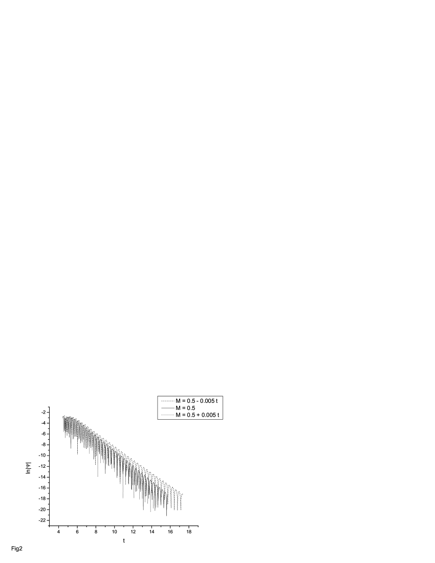
Figure 2: Temporal evolution of the field in the background of a BTZ black hole for $m=10$. The mass of the black hole $M(t)=M_{0}\pm 2At$, where $M_{0}=0.5$ and $2A=5\times 10^{-3}$ are constant coefficients. The field evolution for $M=M_{0}+2At$ and $M=M_{0}-2At$ are shown as the bottom curve and the top curve respectively. For comparison, the oscillation for $M=M_{0}$ is also displayed (the middle curve).

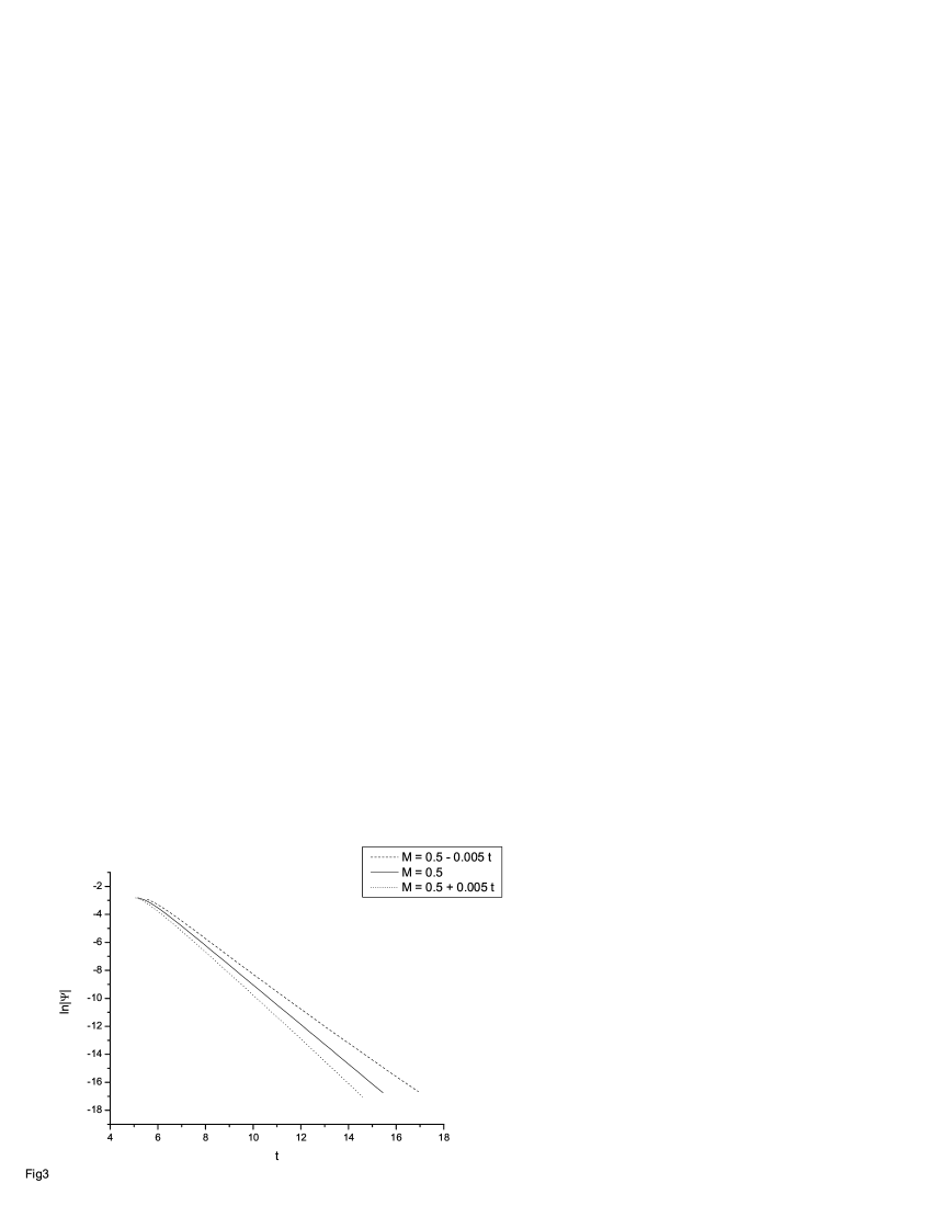
Figure 3: The same plot as Fig. 2. For clarity, the connected maxima of the oscillations are displayed. The imaginary frequency $\omega_{I}$ can be read from the decay time scale $\tau\sim 1/\omega_{I}$.

Figure 4: The frequency $\omega_{R}$ determined from the oscillation period in Fig. 2 is shown as a function of $t$.

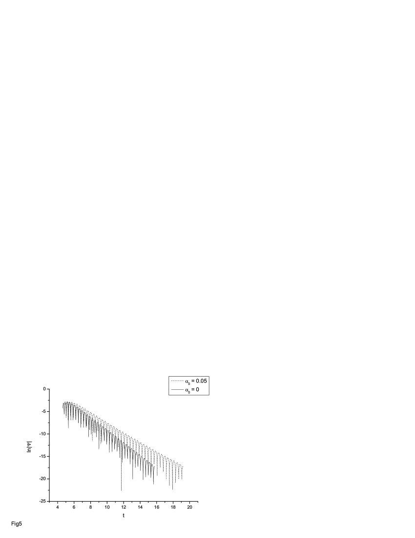
Figure 5: Temporal evolution of the field in the background of a evaporating BTZ black hole (upper curve). We use $\alpha_{0}=0.05$ and $b=2.0$ in our calculation. For comparison, the mode in the stationary background with $M=0.5$ ($\alpha_{0}=0$ and $b=2.0$) is also displayed (lower curve).

Figure 6: Same as Fig. 5. Only the connected maxima of the oscillations are displayed. The imaginary frequency $\omega_{I}$ can be read from the decay time scale $\tau\sim 1/\omega_{I}$.

Figure 7: The frequency $\omega_{R}$ determined from the oscillation period in Fig. 5 is shown as a function of $t$ for the evaporating black hole. For the stationary black hole $\omega_{R}$ is a constant.

References

- (1) K. D. Kokkotas and B. G. Schmidt, Living Rev. Rel. 2, (1999); H. P. Nollert, Class. Quant. Grav. 16, R159 (1999).
- (2) K. D. Kokkotas and B. F. Schwtz, Phys. Rev. D 37, 3378 (1988); N. Andersson, Proc. R. Soc. London A 442, 427 (1993); E. W. Leaver, Phys. Rev. D 41, 2986 (1990).
- (3) R. H. Price, Phys. Rev. D 5, 2419 (1972)
- (4) C. Gundlach, R. H. Price, and J. Pullin, Phys. Rev. D 49, 883 (1994)
- (5) S. Hod and T. Piran, Phys. Rev. D 58, 044018 (1998); R. Moderski and M. Rogatko, Phys. Rev. D 64, 044024 (2001); H. Koyama and A. Tomimatsu, Phys. Rev. D 63, 064032 (2001); L. H. Xue, B. Wang and R. K. Su, Phys. Rev. D 66, 024032 (2002).
- (6) P. R. Brady, C. M. Chambers, W. Krivan and P. Lagunas, Phys. Rev. D 55, 7538 (1997); P. R. Brady, C. M. Chambers, W. G. Laarakkers and E. Poisson, Phys. Rev. D 60, 064003 (1999).
- (7) E. Abdalla, B. Wang, A. Lima-Santos and W. G. Qiu, Phys. Lett. B 538, 435 (2002); E. Abdalla, K. H. C. Castello-Branco and A. Lima-Santos, Phys. Rev. D 66, 104018 (2002).
- (8) J. S. F. Chan and R. B. Mann, Phys. Rev. D 55, 7546 (1999); ibid 59, 064025 (1999).
- (9) G. T. Horowitz and V. E. Hubney, Phys. Rev. D 62, 024027 (2000); G. T. Horowitz, Class. Quant. Grav. 17, 1107 (2000).
- (10) B. Wang, C. Y. Lin and E. Abdalla, Phys. Lett. B 481, 79 (2000); B. Wang, C. Molina and E. Abdalla, Phys. Rev. D 63, 084001 (2001); J. M. Zhu, B. Wang and E. Abdalla, Phys. Rev. D 63, 124004 (2001); B. Wang, E. Abdalla and R. B. Mann, Phys. Rev. D 65, 084006 (2002).
- (11) V. Cardoso and J. P. Lemos, Phys. Rev. D 63, 124015 (2001).
- (12) S. Hod, Phys. Rev. D 66, 024001 (2002).
- (13) L. H. Xue, Z. X. Shen, B. Wang, R. K. Su, gr-qc/0304109
- (14) M. Banados, C. Teitelboim and J. Zanelli, Phy. Rev. Lett 69, 1849 (1992), M. Banados, M. Henneaux, C. Teitelboim, J. Zanelli, Phy. Rev. D 48, 1506 (1993); S. Carlip, Class. Quant. 2853 (1995)
- (15) E. S. C. Ching, P. T. Leung, W. M. Suen and K. Young, Phy. Rev. D 52, 2118 (1995); Phy. Rev. Lett 74, 2414 (1995).
- (16) B. Wang, J. M. Zhu, Mod. Phys. Lett. A 12, 1298 (1995)
- (17) D. Page, Phys. Rev. D 13, 198 (1976); W. A. Hiscock and L. D. Weems, Phys. Rev. D 41, 1142 (1990).