On the exact gravitational lens equation in spherically symmetric and static spacetimes

Abstract

Lensing in a spherically symmetric and static spacetime is considered, based on the lightlike geodesic equation without approximations. After fixing two radius values $r_{O}$ and $r_{S}$, lensing for an observation event somewhere at $r_{O}$ and static light sources distributed at $r_{S}$ is coded in a lens equation that is explicitly given in terms of integrals over the metric coefficients. The lens equation relates two angle variables and can be easily plotted if the metric coefficients have been specified; this allows to visualize in a convenient way all relevant lensing properties, giving image positions, apparent brightnesses, image distortions, etc. Two examples are treated: Lensing by a Barriola-Vilenkin monopole and lensing by an Ellis wormhole.

I Introduction

Theoretical work on gravitational lensing is traditionally done in a quasi-Newtonian approximation formalism, see, e.g., Schneider, Ehlers and Falco Schneider et al. (1992) or Petters, Levine and Wambsganss Petters et al. (2001), which is based, among other things, on the approximative assumptions that the gravitational field is weak and that the bending angles are small. Under these assumptions, lensing is described in terms of a “lens equation” that determines a “lens map” from a “deflector plane” to a “source plane”, thereby relating image positions on the observer’s sky to source positions. Although for all practical purposes up to now this formalism has proven to be very successful, there are two motivations for doing gravitational lens theory beyond the quasi-Newtonian approximation. First, from a methodological point of view it is desirable to investigate qualitative features of lensing, such as criteria for multiple imaging or for the formation of Einstein rings, in a formalism without approximations, as far as possible, to be sure that these features are not just reflections of the approximations. Second, lensing phenomena where strong gravitational fields and large bending angles are involved are no longer as far away from observability as they have been a few years ago. In particular, the discovery that there is a black hole at the center of our galaxy Falcke and Hehl (2003), and probably at the center of most galaxies, has brought the matter of lensing in strong gravitational fields with large bending angles closer to practical astrophysical interest. If a light ray comes sufficiently close to a black hole, the bending angle is not small; in principle, it may even become arbitrarily large, corresponding to the light ray making arbitrarily many turns around the black hole. Unboundedly large bending angles also occur e.g. with wormholes; the latter are more exotic than black holes, in the sense that up to now there is no clear evidence for their existence, but nonetheless considered as hypothetical candidates for lensing by many authors.

If one wants to drop the assumptions of weak fields and small angles, gravitational lensing has to be based on the lightlike geodesic equation in a general-relativistic spacetime, without approximations. In this paper we will discuss this issue for the special case of a spherically symmetric and static spacetime. In view of applications, this includes spherical non-rotating stars and black holes, and also more exotic objects such as wormholes and monopoles with the desired symmetries. The main goal of this paper is to demonstrate that in this case lensing without approximations can be studied, quite conveniently, in terms of a lens equation that is not less explicit than the lens equation of the quasi-Newtonian formalism.

Lensing without weak-field or small-angle approximations was pioneered by Darwin Darwin (1958, 1961) and by Atkinson Atkinson (1965). Whereas Darwin’s work is restricted to the Schwarzschild spacetime throughout, Atkinson derives all relevant formulas for an unspecified spherically symmetric and static spacetime before specializing to the Schwarzschild spacetime in Schwarzschild and in isotropic coordinates. All important features of Schwarzschild lensing are clearly explained in both papers. In particular, they discuss the occurrence of infinitely many images, corresponding to light rays making arbitrarily many turns around the center and coming closer and closer to the light sphere at $r=3m$. However, they do not derive anything like a lens equation.

The notion of a lens equation without weak-field or small-angle approximations was brought forward much later by Frittelli and Newman Frittelli and Newman (1999). It is based on the idea of parametrizing the light cone of an arbitrary observation event in a particular way. For a general discussion of this idea and of the resulting “exact gravitational lens map” in arbitrary spacetimes the reader may consult Ehlers, Frittelli and Newman Ehlers et al. (2003) or Perlick Perlick (2001). Here we are interested only in the special case of a spherically symmetric and static spacetime. Then the geodesic equation is completely integrable and the exact lens equation of Frittelli and Newman can be written quite explicitly. One can evaluate this equation from the spacetime perspective, as has been demonstrated by Frittelli, Kling and Newman Frittelli et al. (2000) for the case of the Schwarzschild spacetime, thereby getting a good idea of the geometry of the light cone. Here we will use an alternative representation, using the symmetry for reducing the dimension of the problem. After fixing two radius values $r_{O}$ and $r_{S}$, lensing for an observation event somewhere at $r_{O}$ and static light sources distributed at $r_{S}$ is coded in a lens equation, explicitly given in terms of integrals over the metric coefficients, that relates two angles to each other. This representation results in a particularly convenient method of visualizing all relevant lensing properties, as will be demonstrated with two examples.

The lens equation discussed in this paper should be compared with the lens equation for spherically symmetric and static spacetimes that was introduced by Virbhadra, Narasimha and Chitre Virbhadra et al. (1998) and then, in a modified form, by Virbhadra and Ellis Virbhadra and Ellis (2000). The Virbhadra-Ellis lens equation has found considerable interest. It was applied to the Schwarzschild spacetime Virbhadra and Ellis (2000) and later also to other spherically symmetric and static spacetimes, e.g. to a boson star by Da̧browski and Schunck Da̧browski and Schunck (2000), to a fermion star by Bilić, Nikolić and Viollier Bilić et al. (2000), to spacetimes with naked singularities by Virbhadra and Ellis Virbhadra and Ellis (2002), to the Reissner-Nordström spacetime by Eiroa, Romero and Torres Eiroa et al. (2002) and to a Gibbons-Maeda-Garfinkle-Horowitz-Strominger black hole by Bhadra Bhadra (2003). In the last two papers, the authors concentrate on light rays that make several turns around the center and they use analytical methods developed by Bozza Bozza (2002). The Virbhadra-Ellis lens equation takes an intermediary position between the exact lens equation and the quasi-Newtonian approximation. It makes no assumptions as to the smallness of bending angles, but it does make approximative assumptions as to the position of light sources and observer. For the Virbhadra-Ellis lens equation to be valid the spacetime must be asymptotically flat for $r\to\infty$ and both observer and light sources must be at positions where $r$ is large; moreover, one has to restrict to light sources close to the radial line opposite to the observer position, i.e., to the case that there is only a small misalignment. (The question of how one can free oneself from the latter assumption was addressed by Da̧browski and Schunck Da̧browski and Schunck (2000) and by Bozza Bozza (2003).) The lens equation to be discussed in the present paper is not restricted to the asymptotically flat case, and it makes no restriction on the position of light sources or observer.

II Derivation of the lens equation

We consider an arbitrary spherically symmetric and static spacetime. For our purpose it will be advantageous to write the metric in the form

$$g\,=\,A(r)^{2}\,\Big{(}\,S(r)^{2}\,dr^{2}\,+\,R(r)^{2}\,(d\vartheta^{2}+{\mathrm{sin}}^{2}\vartheta\,d\varphi^{2})\,-\,dt^{2}\,\Big{)}\,.$$ (1)

Here $\varphi$ and $\vartheta$ are the standard coordinates on the sphere, $t$ ranges over $\mathbb{R}$ and $r$ ranges over an open interval $\;]\,r_{\mathrm{min}}\,,\,r_{\mathrm{max}}\,[\;$ where $-\infty\leq r_{\mathrm{min}}<r_{\mathrm{max}}\leq\infty$. We assume that the functions $A$, $S$, and $R$ are strictly positive and (at least piecewise) differentiable on the interval $\;]\,r_{\mathrm{min}}\,,\,r_{\mathrm{max}}\,[\;$. As the lightlike geodesics are not affected by the conformal factor $A(r)^{2}$ (apart from their parametrizations), the lens equation will depend on the metric coefficients $S(r)$ and $R(r)$ only. We will see below that many qualitative features of the lens equation are determined by the coefficient $R(r)$ alone.

Figure 1: The figure shows the plane $\vartheta=\pi/2$. The observer, indicated by a dot, is situated at $r=r_{O}$, $\varphi=0$, the light sources are distributed at $r=r_{S}$. The lens equation relates the angle $\Theta$ which gives the image position on the observer’s sky to the angle $\Phi$ which gives the source position in the spacetime. The angle $\psi$ indicated in this picture is irrelevant for the lens equation but will be needed in Subsection IV.3.

For introducing our lens equation we have to fix two radius values $r_{O}$ and $r_{S}$ between $r_{\mathrm{min}}$ and $r_{\mathrm{max}}$. The index $O$ stands for “observer”, the index $S$ stands for “source”. We think of an observer at $r=r_{O}$, $\varphi=0$, $\vartheta=\pi/2$. It is our goal to determine the appearance, on the observer’s sky, of static light sources distributed on the sphere $r=r_{S}$.

By symmetry, we may restrict to the plane $\vartheta=\pi/2$. We consider past-oriented lightlike geodesics that start at time $t=0$ at the observer and terminate, at some time $t=-T<0$ which depends on the geodesic, somewhere on the sphere $r=r_{S}$. To each of those light rays we assign the angle $\Theta$, measured at the observer between the ray’s tangent and the direction of $\partial_{r}$, and the angle $\Phi$, swept out by the azimuth coordinate along the ray on its way from the observer to the source, see Figure 1. The desired lens equation is an equation of the form $\mathcal{F}(\Theta,\Phi)=0$ which relates image positions on the observer’s sky, given by $\Theta$, to source positions in the spacetime, given by $\Phi$ modulo $2\pi$. We restrict $\Theta$ to values between $-\pi$ and $\pi$; then $|\Theta|$ can be viewed as a colatitude coordinate on the observer’s celestial sphere. By symmetry, $\mathcal{F}(\Theta,\Phi)=0$ must be equivalent to $\mathcal{F}(-\Theta,-\Phi)=0$. For a given angle $\Theta$, neither existence nor uniqueness of an angle $\Phi$ with $\mathcal{F}(\Theta,\Phi)=0$ is guaranteed. Existence fails if the respective light ray never meets the sphere $r=r_{S}$; uniqueness fails if it meets this sphere several times. In the latter case the observer sees two or more images of light sources at $r_{S}$ at the same point on the sky, one behind the other. We will refer to images which are covered by other images as to “hidden images”. The lens equation can be solved for $\Phi$, thereby giving a lens map $\Theta\mapsto\Phi$, only if hidden images do not exist (or are willfully ignored).

To work out the lens equation we have to calculate the lightlike geodesics in the plane $\vartheta=\pi/2$ of the metric (1), which is an elementary exercise. As a conformal factor has no influence on the lightlike geodesics (apart from their parametrization), they are solutions of the Euler-Lagrange equations of the Lagrangian $\mathcal{L}=\frac{1}{2}\big{(}S(r)^{2}\dot{r}{}^{2}+R(r)^{2}\dot{\varphi}{}^{2}-\dot{t}{}^{2}\big{)}$, i.e.

$$\big{(}S(r)^{2}\dot{r}\big{)}\dot{\,}\,=\,S(r)\,S\,^{\prime}(r)\,\dot{r}{}^{2}\,+\,R(r)\,R\,^{\prime}(r)\,\dot{\varphi}{}^{2}\;,$$ (2)

$$\big{(}R(r)^{2}\dot{\varphi}\big{)}\dot{\,}\,=\,0\;,$$ (3)

$$\ddot{t}\,=\,0\;,$$ (4)

where an overdot denotes differentiation with respect to the curve parameter $s$. As an aside we mention that, by (2), a circular light ray exists at radius $r_{p}$ if and only if $R^{\prime}(r_{p})=0$. Comparing this condition with the equivalent but less convenient eq. (33) in Atkinson’s article Atkinson (1965) shows that it is advantageous to write the metric in the form (1). The relevance of circular light rays in view of lensing was discussed by Hasse and Perlick Hasse and Perlick (2002), also see Claudel, Virbhadra and Ellis Claudel et al. (2001) for related results.

To get the past-oriented light ray that starts at time $t=0$ at the observer in the direction determined by the angle $\Theta$ we have to impose the initial conditions

$$r|_{s=0}\,=\,r_{O}\;,\qquad\dot{r}|_{s=0}\,=\,\frac{\mathrm{cos}\,\Theta}{S(r_{O})}\;,$$ (5)

$$\varphi|_{s=0}\,=\,0\;,\qquad\dot{\varphi}|_{s=0}\,=\,\frac{\mathrm{sin}\,\Theta}{R(r_{O})}\;,$$ (6)

$$t|_{s=0}\,=\,0\;,\qquad\dot{t}|_{s=0}\,=\,-\,1\;.$$ (7)

For each $\Theta$, the initial value problem (2), (3), (4),(5), (6), (7) has a unique maximal solution

$$r=\mathsf{r}(\Theta,s)\;,\qquad\varphi=\phi(\Theta,s)\;,\qquad t=-s$$ (8)

where $s$ ranges from 0 up to some $s_{\mathrm{max}}(\Theta)$. Every image on the oberver’s sky of a light source at $r_{S}$ corresponds to a pair $(\Theta,\Phi)$ such that

$$r_{S}=\mathsf{r}(\Theta,T)\qquad\text{and}\qquad\Phi=\phi(\Theta,T)$$ (9)

with some parameter value $T\in\;]\,0,s_{\mathrm{max}}(\Theta)\,[\>$. In other words, we get the desired lens equation $\mathcal{F}(\Theta,\Phi)=0$ if we eliminate $T$ from the two equations (9).

We get an explicit expression for the lens equation, and for the travel time $T$, by writing the functions $\mathsf{r}(\Theta,s)$ and $\phi(\Theta,s)$ in terms of integrals. From the constant of motion

$$S(r)^{2}\,{\dot{r}}{}^{2}\,+\,R(r)^{2}\,{\dot{\varphi}}{}^{2}\,-\,{\dot{t}}{}^{2}\,=\,0$$ (10)

we find, with the help of (3), (4),(6), (7),

$$S(r)^{2}\,R(r)^{2}\,\dot{r}{}^{2}\,=\,R(r)^{2}-R(r_{O})^{2}{\mathrm{sin}}^{2}\Theta\;.$$ (11)

If $\dot{r}$ does not change sign, integration of (11) yields

$$s\,=\,\frac{|\mathrm{cos}\,\Theta|}{\mathrm{cos}\,\Theta}\,\int_{r_{O}}^{\mathsf{r}(\Theta,s)}\frac{R(r)\,S(r)\,dr}{\sqrt{R(r)^{2}-R(r_{O})^{2}\,\mathrm{sin}^{2}\Theta}}\>.$$ (12)

With $\mathsf{r}(\Theta,s)$ known, $\varphi=\phi(\Theta,s)$ is determined by integrating (3) with (6),

$$\phi(\Theta,s)\,=\,\int_{0}^{s}\frac{R(r_{O})\,\mathrm{sin}\,\Theta\,d\tilde{s}}{R\big{(}\mathsf{r}(\Theta,\tilde{s})\big{)}^{2}}\>.$$ (13)

(13) can be rewritten as an integral over $r$, with $\dot{r}=dr/ds$ substituted from (11). This gives us the lens equation in the form

$$\Phi\,=\,\frac{|\mathrm{cos}\,\Theta|}{\mathrm{cos}\,\Theta}\,\int_{r_{O}}^{r_{S}}\frac{R(r_{O})\,\mathrm{sin}\,\Theta\,S(r)\,dr}{R(r)\,\sqrt{R(r)^{2}-R(r_{O})^{2}\mathrm{sin}^{2}\Theta}}\>.$$ (14)

If $\dot{r}$ changes sign, (12) has to be replaced by a piecewise integration. Similarly, the substitution from the $s$-integration in (13) to an $r$-integration must be done piecewise. In this case, the lens equation is not of the form (14); in particular, it is not guaranteed that the lens equation can be solved for $\Phi$. In any case, we get exact integral expressions for the lens equation, and for the travel time $T$, from which all relevant lensing features can be determined in a way that is not less explicit than the quasi-Newtonian approximation formalism. This will be demonstrated by two examples in Section V. In Subsection V.1 we treat a particularly simple example where the metric coefficients $R(r)$ and $S(r)$ are analytic and the integral (12) can be explicitly calculated in terms of elementary functions. In this case it suffices to calculate (12) for arbitrarily small $s$ to get the whole function $r(\Theta,s)$ by maximal analytic extension; i.e., in this case it is not necessary to determine the points where $\dot{r}$ changes sign and to perform a piecewise integration.

III Discussion of the lens equation

In the first part of this section we want to discuss for which values of $\Theta$ the lens equation $\mathcal{F}(\Theta,\Phi)=0$ admits a solution. In other words, we want to determine which part of the observer’s sky is covered by the light sources distributed at $r=r_{S}$. We restrict to the case $r_{O}<r_{S}$. (The results for the case $r_{O}>r_{S}$ follow immediately from our discussion; we just have to make a coordinate transformation $r\to-r$ and, correspondingly, to change $\Theta$ into $\pi-\Theta$. The case $r_{O}=r_{S}$ can be treated by a limit procedure.)

For a light ray with one end-point at $r_{O}$ and the other at $r_{S}$ the right-hand side of (11) must be non-negative for all $r$ between $r_{O}$ and $r_{S}$. This condition restricts the possible values of $\Theta$ by $\mathrm{sin}^{2}\Theta\leq\mathrm{sin}^{2}\delta_{I}$ where

$$\mathrm{sin}\,\delta_{I}\,=\,{\mathrm{inf}}\,\big{\{}\,R(r)/R(r_{O})\,\big{|}\,r_{O}<r<r_{S}\,\big{\}}\;.$$ (15)

Note that our assumptions guarantee that this infimum is strictly positiv, $0<\delta_{I}\leq\pi/2$.

Furthermore, a light ray with $\pi/2<|\Theta|<\pi$ can arrive at $r_{S}$ only if it passes through a minimal radius value $\rho(\Theta)<r_{O}$. As (11) requires $R\big{(}\rho(\Theta)\big{)}^{2}=R(r_{O})^{2}\mathrm{sin}^{2}\Theta$, this can be true only if $\mathrm{sin}^{2}\Theta\geq\mathrm{sin}^{2}\delta_{II}$ where

$$\mathrm{sin}\,\delta_{II}\,=\,{\mathrm{inf}}\,\big{\{}\,R(r)/R(r_{O})\,\big{|}\,r_{\mathrm{min}}<r<r_{O}\,\big{\}}\;,$$ (16)

$0\leq\delta_{II}\leq\pi/2$. So in general the light sources at $r_{S}$ cover on the observer’s sky a disk of angular radius $\delta_{I}$ around the pole $\Theta=0$ and, if $\delta_{II}<\delta_{I}$, in addition a ring of angular width $\delta_{I}-\delta_{II}$ around the pole $\Theta=\pi\simeq-\pi$, see Figure 2. The two domains join if $\delta_{I}=\pi/2$.

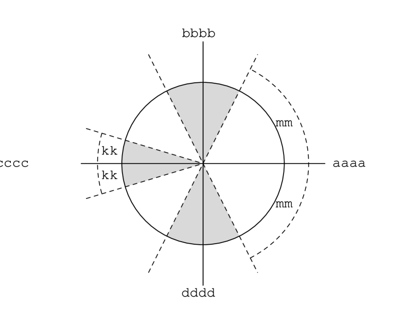
Figure 2: In the case $r_{O}<r_{S}$, the light sources cover the non-shaded region on the observer’s sky, with $\delta_{I}$ and $\delta_{II}$ given by (15) and (16), respectively. (For $r_{S}<r_{O}$ one gets an analogous picture, with $\Theta=0$ and $\Theta=\pi\simeq-\pi$ interchanging their roles.) If the spacetime is asymptotically flat and if $r_{S}$ is sufficiently large, this picture gives the socalled “escape cones” which have been calculated by Synge Synge (1966) for the Schwarzschild spacetime and by Pande and Durgapal Pande and Durgapal (1986) for an unspecified asymptotically flat spherically symmetric and static spacetime.

We see that the allowed values of $\Theta$ are determined by the metric coefficient $R$ alone. We will now demonstrate that $R$ alone also determines the occurrence or non-occurrence of hidden images. Hidden images occur if a light ray from $r_{O}$ intersects the sphere $r=r_{S}$ at least two times; between these two intersections it must pass through a maximal radius $\sigma(\Theta)>r_{S}$ which, by (11), has to satisfy $R\big{(}\sigma(\Theta)\big{)}^{2}=R(r_{O})^{2}\mathrm{sin}^{2}\Theta$. Such a radius $\sigma(\Theta)$ exists for all $\Theta$ with $\mathrm{sin}^{2}\Theta>C^{2}$ where

$$C\,=\,{\mathrm{inf}}\,\big{\{}\,R(r)/R(r_{O})\,\big{|}\,r_{S}<r<r_{\mathrm{max}}\,\big{\}}\;.$$ (17)

As $\Theta$ is restricted by $\mathrm{sin}^{2}\Theta\leq\mathrm{sin}^{2}\delta_{I}$, hidden images cannot occur if $C\geq\mathrm{sin}\,\delta_{I}$. The latter condition is satisfied in asymptotically flat spacetimes, where $R(r)\to\infty$ for $r\to r_{\mathrm{max}}\,(=\infty)$, if we choose $r_{S}$ sufficiently large. This is the reason why in the more special situation of the Virbhadra-Ellis lens equation Virbhadra and Ellis (2000) hidden images cannot occur.

In the rest of this section we discuss the question of multiple imaging and the occurrence of Einstein rings. For a light source at $r=r_{S}$, $\varphi=\varphi_{0}$, $\vartheta=\pi/2$ with $0<|\varphi_{0}|<\pi$, images on the observer’s sky are in one-to-one correspondence with solutions $\Theta$ of the equation

$$\mathcal{F}\big{(}\Theta,\varphi_{0}\,+\,2\,n\,\pi\big{)}\,=\,0$$ (18)

with $n\in\mathbb{Z}$. We call the integer $n$ the “winding number” of the corresponding light ray. An image with $n=0$ is called “primary” and an image with $n=-\varphi_{0}/|\varphi_{0}|$ is called “secondary”. Images with other values of $n$ correspond to light rays that make at least one full turn and have been termed “relativistic” by Virbhadra and Ellis Virbhadra and Ellis (2000). Note that different images of a light source may have the same winding number.

If we send $\varphi_{0}$ to 0 or to $\pi\simeq-\pi$, solutions $\Theta$ of equation (18) with $\mathrm{sin}\,\Theta\neq 0$ come in pairs $(\Theta,-\Theta)$. By spherical symmetry, every such pair gives rise to an Einstein ring. There are as many Einstein rings as the equation

$$\mathcal{F}(\Theta,i\,\pi)\,=\,0$$ (19)

admits solutions with positive integers $i$. Even integers $i$ correspond to Einstein rings of the source at $\varphi_{0}=0$, and odd integers $i$ correspond to Einstein rings of the source at $\varphi_{0}=\pi\simeq-\pi$.

IV Observables

To each solution $(\Theta,\Phi)$ of the lens equation we can assign redshift, travel time, apparent brightness and image distortion.

IV.1 Redshift

The general redshift formula for static metrics (see, e.g., Straumann Straumann (1984), p. 97) specified to metrics of the form (1) says that the redshift $z$ is given by

$$1\,+\,z\,=\,\frac{\,A(r_{O})\,}{A(r_{S})}$$ (20)

if the observer’s worldline is a $t$-line at $r=r_{O}$ and the source’s worldline is a $t$-line at $r=r_{S}$. In our situation $r_{O}$ and $r_{S}$ are fixed, so the redshift is a constant.

IV.2 Travel time

Recall that $(\Theta,\Phi)$ is a solution of the lens equation if and only if there is a parameter $T$ such that the equations (9) hold. This assigns a travel time $T$ to each solution $(\Theta,\Phi)$ of the lens equation. If there are no hidden images, the equation $\mathsf{r}(\Theta,T)=r_{S}$ gives $T$ as a single-valued function of $\Theta$.

IV.3 Angular diameter distance

Quite generally, determination of the angular diameter distance requires solving the Sachs equations for the optical scalars along lightlike geodesics, see e.g. Schneider, Ehlers and Falco Schneider et al. (1992). For the Schwarzschild metric, this has been explicitly worked out by Dwivedi and Kantowski Dwivedi and Kantowski (1972). Their method easily carries over to arbitrary spherically symmetric and static spacetimes as was demonstrated by Dyer Dyer (1977). In what follows we give a reformulation of these results in terms of our lens equation.

To that end we fix a solution $(\Theta,\Phi)$ of the lens equation and thereby a (past-oriented) light ray from the observer at $r_{O}$ to a light source at $r_{S}$. Around this ray, we consider an infinitesimally thin bundle of neighboring rays, with vertex at the observer. The angular diameter distance is defined as the square-root of the ratio between the cross-sectional area of this bundle at the light source and the opening solid angle at the observer. Owing to the symmetry of our situation there are two preferred spatial directions perpendicular to the ray: a radial direction (along a meridian on the observer’s sky) and a tangential direction (along a circle of equal latitude on the observer’s sky). Therefore, the angular diameter distance naturally comes about as a product of a radial part and a tangential part.

To calculate the radial part, we consider the infinitesimally neighboring ray which corresponds to an infinitesimally neighboring solution $(\Theta+d\Theta,\Phi+d\Phi)$ of the lens equation, i.e. $d\Phi$ and $d\Theta$ satisfy

$$\frac{\partial\mathcal{F}}{\partial\Theta}(\Theta,\Phi)\,+\,\frac{\partial\mathcal{F}}{\partial\Phi}(\Theta,\Phi)\,\frac{d\Phi}{d\Theta}\>=\>0$$ (21)

We define the radial angular diameter distance as

$$D^{r}_{\mathrm{ang}}\,=\,A(r_{S})\,R(r_{S})\,\mathrm{cos}\,\psi\,\frac{d\Phi}{d\Theta}$$ (22)

with $\psi$ given by Figure 1, i.e., $A(r_{S})\,R(r_{S})\,\mathrm{cos}\,\psi\,d\Phi$ measures, in the direction perpendicular to the original ray, how far the neighboring ray is away. By (3), (6) and (11), $\psi$ must satisfy

$$R(r_{O})\,\mathrm{sin}\,\Theta\,=\,R(r_{S})\,\mathrm{sin}\,\psi\,.$$ (23)

With $\psi$ given by (23) and $d\Phi/d\Theta$ given by (21), $D^{r}_{\mathrm{ang}}$ is determined by (22) for every solution $(\Theta,\Phi)$ of the lens equation. Note that $D^{r}_{\mathrm{ang}}$ is singular at those solutions of the lens equation where $\partial\mathcal{F}/\partial\Phi$ has a zero. If the lens equation can be solved for $\Phi$, we may view $D^{r}_{\mathrm{ang}}$ as a (single-valued) function of $\Theta$.

To calculate the tangential part we consider an infinitesimally neighboring light ray that results by applying a rotation around the axis $\varphi=0$, $\vartheta=\pi/2$. Such rotations are generated by the Killing vector field $K=\mathrm{sin}\,\varphi\,\partial_{\vartheta}+\mathrm{cot}\,\vartheta\,\mathrm{cos}\,\varphi\,\partial_{\varphi}$. At points with $\vartheta=\pi/2$, this Killing vector field takes the form $K\,=\mathrm{sin}\,\varphi\,A(r)\,R(r)\,g(\partial_{\vartheta},\partial_{\vartheta})^{-1/2}\,\partial_{\vartheta}$. Hence, if we rotate by an infinitesimal angle $d\beta$, the neighboring ray intersects the sphere $r=r_{S}$ at a distance $A(r_{S})\,R(r_{S})\,\mathrm{sin}\,\Phi\,d\beta$ from the original ray. Relating this distance to the angle $\mathrm{sin}\,\Theta\,d\beta$ between the two rays at the observer gives the tangential angular diameter distance

$$D^{t}_{\mathrm{ang}}\,=\,A(r_{S})\,R(r_{S})\,\frac{\,\mathrm{sin}\,\Phi\,}{\mathrm{sin}\,\Theta}\;.$$ (24)

By this equation, $D^{t}_{\mathrm{ang}}$ is uniquely determined for each solution $(\Theta,\Phi)$ of the lens equation. Again, $D^{t}_{\mathrm{ang}}$ may be viewed as a function of $\Theta$ if the lens equation can be solved for $\Phi$.

$D^{r}_{\mathrm{ang}}$ and $D^{t}_{\mathrm{ang}}$ together give the (averaged) angular diameter distance or area distance

$$D_{\mathrm{ang}}\,=\,\sqrt{\,|D^{r}_{\mathrm{ang}}\,D^{t}_{\mathrm{ang}}|\,}\;.$$ (25)

Note that both $D^{r}_{\mathrm{ang}}$ and $D^{t}_{\mathrm{ang}}$ may be negative. Images with $D^{r}_{\mathrm{ang}}\,D^{t}_{\mathrm{ang}}\,>\,0$ are said to have even parity and images with $D^{r}_{\mathrm{ang}}\,D^{t}_{\mathrm{ang}}\,<\,0$ are said to have odd parity. Images with odd parity show the neighborhood of the light source side-inverted in comparison to images with even parity.

A solution $(\Theta,\Phi)$ of the lens equation is called a radial critical point if $D^{r}_{\mathrm{ang}}=0$ and a tangential critical point if $D^{t}_{\mathrm{ang}}=0$. The latter condition is equivalent to $\mathrm{sin}\,\Phi=0$ and $\mathrm{sin}\,\Theta\neq 0$, i.e., to the occurrence of an Einstein ring. Note that (radial and tangential) critical points come in pairs, $(\Theta,\Phi)$ and $(-\Theta,-\Phi)$. Every such pair corresponds to a circle of equal latitude on the observer’s sky which may be called a (radial or tangential) critical circle, as in the quasi-Newtonian approximation formalism, see Schneider, Ehlers and Falco Schneider et al. (1992), p. 233. In the quasi-Newtonian formalism one usually introduces the inverse magnification factors $1/\mu^{r}$ and $1/\mu^{t}$ as substitutes for $D^{r}_{\mathrm{ang}}$ and $D^{t}_{\mathrm{ang}}\,$. In our situation, where there is no flat background metric, not even asymptotically, the magnification factors cannot be defined in a reasonable way, but working with $D^{r}_{\mathrm{ang}}$ and $D^{t}_{\mathrm{ang}}\,$ is completely satisfactory.

IV.4 Luminosity distance

In arbitrary spacetimes, the angular diameter distance $D_{\mathrm{ang}}$ is related to the (uncorrected) luminosity distance $D_{\mathrm{lum}}$ by the universal formula $D_{\mathrm{lum}}=(1+z)^{2}D_{\mathrm{ang}}$, see, e.g., Schneider, Ehlers and Falco Schneider et al. (1992) , eq. (3.80). With the redshift $z$ given by (20) and the angular diameter distance $D_{\mathrm{ang}}$ given by (25), we find

$$D_{\mathrm{lum}}\,=\,\frac{\,A(r_{O})^{2}\,}{A(r_{S})^{2}}\,\sqrt{\,|D^{r}_{\mathrm{ang}}\,D^{t}_{\mathrm{ang}}|\,}\;.$$ (26)

For an isotropically radiating light source with bolometric luminosity $L$, the total flux at the observer is $L/(4\pi D_{\mathrm{lum}}^{2})$, see again Schneider, Ehlers and Falco Schneider et al. (1992), eq. (3.79). Hence, if we distribute standard candles at $r=r_{S}$, their apparent brightness on the observer’s sky is proportional to $D_{\mathrm{lum}}^{-2}$.

IV.5 Image distortion

$D^{r}_{\mathrm{ang}}$ and $D^{t}_{\mathrm{ang}}$ immediately give the apparent distortion of images. For the sake of illustration, we may think of small spheres, with infinitesimal diameter $dD$, distributed with their centers at $r=r_{S}$. By definition of $D^{r}_{\mathrm{ang}}$ and $D^{t}_{\mathrm{ang}}$, each solution $(\Theta,\Phi)$ of the lens equation corresponds to an elliptical image of such a sphere on the observer’s sky, with the radial (meridional) diameter of the ellipse equal to $|d\Theta|=|dD/D^{r}_{\mathrm{ang}}|$ and with the tangential (latitudinal) diameter of the ellipse equal to $|d\beta|=|dD/D^{t}_{\mathrm{ang}}|$. Thus, we may use the ellipticity

$$\varepsilon\;=\;\frac{\,|d\Theta|\,-\,|d\beta|\,}{|d\Theta|\,+\,|d\beta|}\;=\;\frac{\,|D^{r}_{\mathrm{ang}}|\,-\,|D^{t}_{\mathrm{ang}}|\,}{\,|D^{r}_{\mathrm{ang}}|\,+\,|D^{t}_{\mathrm{ang}}|}$$ (27)

as a measure for image distortion.

V Examples

V.1 Lensing by a Barriola-Vilenkin monopole

We consider the metric

$$g\,=\,dr^{2}\,+\,k^{2}\,r^{2}\,(d\vartheta^{2}+{\mathrm{sin}}^{2}\vartheta\,d\varphi^{2})\,-\,dt^{2}\,$$ (28)

where $k$ is a positive constant. For $k=1$, this is just Minkowski spacetime in spherical coordinates. For $k<1$, there is a deficit solid angle and a singularity at $r=0\,$; the plane $t={\mathrm{const.}}$, $\vartheta=\pi/2$ has the geometry of a cone. Similarly, for $k>1$ there is a surplus solid angle and a singularity at $r=0$. For $k\neq 1$, the metric is non-flat. The Einstein tensor has non-vanishing components $G_{tt}\,=\,-\,G_{rr}\,=\,(1-k^{2})/r^{2}$, so the weak energy condition is satisfied (without a cosmological constant) if and only if $k\leq 1$. In that case it was shown by Barriola and Vilenkin Barriola and Vilenkin (1989) that the metric may be viewed as a model for the spacetime around a monopole resulting from breaking a global $O(3)$ symmetry. To within the weak-field approximation, basic features of lensing by such a monopole were discussed in the original paper by Barriola and Vilenkin Barriola and Vilenkin (1989) and also by Durrer Durrer (1994). In what follows we give a detailed account in terms of our exact lens equation. Note that the Virbhadra-Ellis lens equation Virbhadra and Ellis (2000) is not applicable to this case, at least not without modification, because for $k\neq 1$ the spacetime is not asymptotically flat in the usual sense.

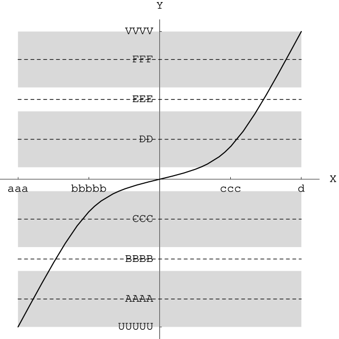
Figure 3: The lens equation (32) for the Barriola-Vilenkin monopole with $k=1/3.7$ and $r_{O}=0.77\,r_{S}$. Intersections with the dashed lines indicate Einstein rings. Shading distinguishes sources with $N(k)+1=4$ images from sources with $N(k)=3$ images.

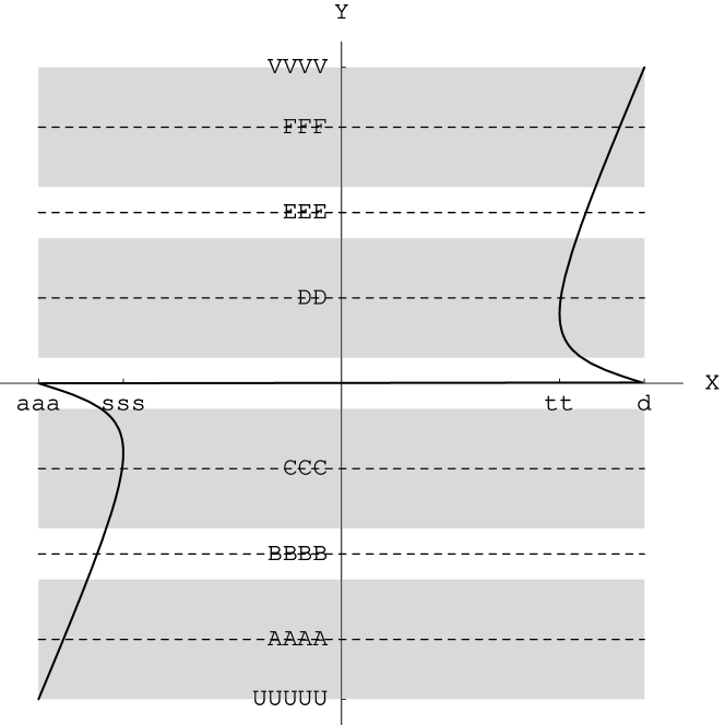
Figure 4: The lens equation (32) for the Barriola-Vilenkin monopole with $k=1/3.7$ and $r_{S}=0.77\,r_{O}$. Other than in the case $r_{O}<r_{S}$, the lens equation cannot be solved for $\Phi$, i.e., there are hidden images. The angle $\alpha$ is determined by $r_{S}\,=\,r_{O}\,\mathrm{sin}\,\alpha$ and $\pi/2<\alpha<\pi$. The picture shows that all Einstein rings, indicated by intersections with the dashed lines, are hidden. Shading distinguishes sources with $N(k)+1=4$ images from sources with $N(k)=3$ images; only one image of each source is non-hidden.

Figure 5: Tangential angular diameter distance $D_{\mathrm{ang}}^{r}$ (dashed) and radial angular diameter distance $D_{\mathrm{ang}}^{t}$ (solid) as functions of $\Theta$ for the Barriola-Vilenkin monopole with $k=1/3.7$ and $r_{O}=0.77\,r_{S}$. The dashed curve also gives the travel time $T=D_{\mathrm{ang}}^{r}$. Each zero of $D_{\mathrm{ang}}^{t}$ indicates an Einstein ring. Where $D_{\mathrm{ang}}^{t}$ and $D_{\mathrm{ang}}^{r}$ have the same sign, the images have even parity; where $D_{\mathrm{ang}}^{t}$ and $D_{\mathrm{ang}}^{r}$ have different signs, the images have odd parity, i.e., the neighborhood of each light source is shown side-inverted.

Comparison of (28) with (1) shows that the metric coefficients are given by

$$A(r)\,=\,1\;,\qquad S(r)\,=\,1\;,\qquad R(r)\,=\,k\,r$$ (29)

on the interval $r_{\mathrm{min}}=0<r<r_{\mathrm{max}}=\infty$. With these metric coefficients, the integrals (12) and (13) can be calculated in an elementary fashion, yielding the solution to the initial value problem in the form

$$\mathsf{r}(\Theta,s)\,=\,\sqrt{\,r_{O}^{2}\,+\,2\,r_{O}\,s\,\mathrm{cos}\,\Theta\,+\,s^{2}\,}\>,$$ (30)

$$\phi(\Theta,s)\,=\,\frac{1}{k}\,\frac{\,\mathrm{sin}\,\Theta\,}{|\mathrm{sin}\,\Theta|}\,\mathrm{arccos}\Big{(}\frac{\,r_{O}\,+\,s\,\mathrm{cos}\,\Theta}{\sqrt{\,r_{O}^{2}\,+\,2\,r_{O}\,s\,\mathrm{cos}\,\Theta\,+\,s^{2}\,}}\Big{)}\>.$$ (31)

For $\mathrm{sin}\,\Theta\,\neq\,0\,$, $s$ ranges from 0 to $\infty$, so $|\varphi|=|\phi(\Theta,s)|$ ranges from 0 to $|\Theta|/k$. Eliminating $T$ from the two equations (9) gives the lens equation,

$$r_{S}\,\mathrm{sin}(\Theta-k\Phi)\,-\,r_{O}\,\mathrm{sin}\,\Theta\>=\>0\;,$$ (32)

which is to be considered on the domain

$$-\pi<\Theta<\pi\>,\qquad k|\Phi|<|\Theta|\>.$$ (33)

We restrict to the case that the integer $N(k)$ defined by $N(k)\leq 1/k<N(k)+1$ is odd. The lens equation is plotted for the case $r_{O}<r_{S}$ in Figure 3 and for the case $r_{O}>r_{S}$ in Figure 4. (For producing the pictures we have chosen $k$ such that $N(k)=3$.) In either case we find that there are $N(k)$ Einstein rings. For a light source at $r=r_{S},\varphi=\varphi_{0},\vartheta=\pi/2$ with $0<|\varphi_{0}|<\pi$ there are $N(k)$ images if $|\varphi_{0}|\leq\big{(}1+N(k)-1/k\big{)}\pi$ (non-shaded regions in Figures 3 and 4) and $N(k)+1$ images otherwise (shaded regions in Figures 3 and 4).

Figure 6: Apparent brightness of standard candles for the Barriola-Vilenkin monopole with $k=1/3.7$ and $r_{O}=0.77\,r_{S}$. Instead of $D_{\mathrm{lum}}^{-2}$, which is proportional to the energy flux from point sources, we have plotted the magnitude $m=2.5\,\mathrm{log}_{10}(D_{\mathrm{lum}}^{2})+m_{0}$ used by astronomners. The constant $m_{0}$ has been chosen such that $m=0$ at $\Theta=0$. Einstein rings are infinitely bright in the ray optical treatment, $m=-\infty$.

In the following we concentrate on the case $r_{O}<r_{S}$. Then the lens equation can be solved for $\Phi$, giving a lens map

$$\Theta\>\longmapsto\>\Phi\,=\,\frac{1}{k}\,\left(\,\Theta\,-\,\mathrm{arcsin}\Big{(}\,\frac{r_{O}}{r_{S}}\,\mathrm{sin}\,\Theta\,\Big{)}\right)$$ (34)

on the domain $-\pi<\Theta<\pi$, i.e., in the notation of Figure 2 we have $\delta_{I}=\pi/2$ and $\delta_{II}=0$. In the case $k=1$ (flat spacetime), the lens map can be continuously extended into the point $\Theta=\pi\simeq-\pi$ (and by periodicity onto the full circle, $\Theta\in\mathbb{R}$ mod $2\pi$). For $k\neq 1$ the ray with $\Theta=\pi\simeq-\pi$ cannot pass through the singularity at $r=0$, so the lens map is not to be extended beyond the open interval $\,\>]-\pi,\pi\,[\>\,$. On this interval, $\Phi$ increases monotonously from $-\pi/k$ to $\pi/k$, see Figure 3. Thus, the range of the lens map is independent of $r_{O}$ and $r_{S}$. The ratio $r_{O}/r_{S}$ influences the shape of the graph of the lens map in the following way. For $r_{O}/r_{S}\to 0$ it becomes a straight line, $\Phi=\Theta/k$. For $r_{O}/r_{S}\to 1$ it becomes a broken straight line, $\Phi=0$ for $|\Theta|\leq\pi/2$ and $\Phi=(2\Theta-\pi)/k$ for $|\Theta-\pi|<\pi/2$. Note that linearity of the lens map implies that the angular distance on the observer’s sky between consecutive images is the same for all light sources.

Figure 7: The ellipticity $\varepsilon$ for the Barriola-Vilenkin monopole with $k=1/3.7$ and $r_{O}=0.77\,r_{S}$. If small spheres are distributed with their centers at $r=r_{S}$, this function describes their distortion into ellipses on the observer’s sky. $\varepsilon=0$ indicates circular images, $\varepsilon=-1$ images with no tangential extension (radial critical points), and $\varepsilon=1$ images with no radial extension (tangential critical points, i.e. Einstein rings).

As $\Phi$ is a (single-valued) function of $\Theta$, so are all observables. By evaluating the formulas derived in Section IV for the case at hand we find

$$z\,=\,0\>,$$ (35)

$$T\,=\,D_{\mathrm{ang}}^{r}\,=\,r_{O}\,\mathrm{cos}\,\Theta\,+\,\sqrt{\,r_{S}^{2}\,-\,r_{O}^{2}\mathrm{sin}^{2}\Theta\,}\>,$$ (36)

$$D_{\mathrm{ang}}^{t}\,=\,\frac{k\,r_{S}}{\,\mathrm{sin}\,\Theta\,}\>\mathrm{sin}\left(\,\frac{1}{k}\,\Big{(}\,\Theta\,-\,\mathrm{arcsin}\big{(}\,\frac{r_{O}\,\mathrm{sin}\,\Theta\,}{r_{S}}\,\big{)}\Big{)}\right)\>,$$ (37)

which gives $D_{\mathrm{lum}}$ and $\varepsilon$ as functions of $\Theta$ via (26) and (27). The observables are plotted in Figures 5, 6 and 7.

V.2 Lensing by an Ellis wormhole

The metric

$$g\,=\,dr^{2}\,+\,(r^{2}+a^{2})\,(d\vartheta^{2}+{\mathrm{sin}}^{2}\vartheta\,d\varphi^{2})\,-\,dt^{2}\;,$$ (38)

where $a$ is a positive constant, is an example for a traversable wormhole of the Morris-Thorne class, see Box 2 in Morris and Thorne Morris and Thorne (1988). It was investigated, already in the 1970s, by Ellis Ellis (1973) who called it a “drainhole”. Lensing in the Ellis spacetime was discussed, in a scattering formalism assuming that observer and light source are at infinity, by Chetouani and Clément Chetouani and Clément (1984). In the following we give a detailed account of lensing in this spacetime with the help of our lens equation.

By comparison of (38) with (1) we find

$$A(r)\,=\,1\;,\qquad S(r)\,=\,1\;,\qquad R(r)\,=\,\sqrt{r^{2}+a^{2}}\,.$$ (39)

where the radius coordinate $r$ ranges from $r_{\mathrm{min}}=-\infty$ to $r_{\mathrm{max}}=\infty$. (We do not identify the region where $r$ is positive with the region where $r$ is negative.) The function $R$ has a minimum at $r=0$, thereby indicating the existence of circular light rays at the neck of the wormhole. In the following we consider the case that observer and light sources are on different sides of the neck of the wormhole, $-\infty<r_{O}<0<r_{S}<\infty$.

Figure 8: The lens equation (42) for the Ellis wormhole. The angle $\delta_{I}(<\pi/2)$ is defined in (40). There are infinitely many Einstein rings, indicated by intersections with the dashed lines.

Figure 9: The travel time $T$ as a function of $\Theta$ for the Ellis wormhole. The axis $\Theta=0$ is met at $T_{0}=r_{S}-r_{O}$, see (44).

As a first step, we determine for which angles $\Theta$ the lens equation admits a solution, recall Figure 2. In the case at hand, the angles $\delta_{I}$ and $\delta_{II}$ defined by (15) and (16) are given by $\mathrm{sin}\,\delta_{I}=a/\sqrt{r_{O}^{2}+a^{2}}$ and $\delta_{II}=\pi/2>\delta_{I}$. Hence, the lens equation admits a solution for all angles $\Theta$ with $|\Theta|<\pi/2$ and

$${\mathrm{sin}}^{2}\Theta\,<\,\mathrm{sin}^{2}\delta_{I}\,=\,\frac{a^{2}}{r_{O}^{2}+a^{2}}\;.$$ (40)

Light sources distributed at $r=r_{S}$ illuminate a disk of angular radius $\delta_{I}<\pi/2$ on the observer’s sky. The apparent rim of the disk corresponds to light rays that spiral asymptotically towards $r=0$. As the constant $C$ defined by (17) satisfies $C\,=\,\sqrt{(r_{S}^{2}+a^{2})/(r_{O}^{2}+a^{2})}\,>\,a/\sqrt{r_{O}^{2}+a^{2}}\,=\,\mathrm{sin}\,\delta_{I}$, there are no hidden images, i.e., the lens equation can be solved for $\Phi$.

Figure 10: $D_{\mathrm{ang}}^{r}$ (dashed) and $D_{\mathrm{ang}}^{t}$ (solid) as functions of $\Theta$ for the Ellis wormhole. At each Einstein ring $D_{\mathrm{ang}}^{t}$ has a zero. To make the oscillatory behaviour of $D_{\mathrm{ang}}^{t}$ visible, we use $x=-\mathrm{log}\big{(}1-|\Theta|/\delta_{I}\big{)}$ instead of $\Theta$ on the abscissa; $|\Theta|$ ranges from 0 to $\delta_{I}$ if $x$ ranges from 0 to $\infty$. The axis is met at $D_{0}=\sqrt{r_{S}^{2}+a^{2}}\sqrt{r_{O}^{2}+a^{2}}\,a^{-1}\big{(}\mathrm{arctan}(r_{S}/a)-\mathrm{arctan}(r_{O}/a)\big{)}$, see (45) and (46).

Figure 11: The apparent brightness, measured in terms of magnitude $m=2.5\,\mathrm{log}_{10}(D_{\mathrm{lum}}^{2})+m_{0}$, as a function of $\Theta$ for the Ellis wormhole. The constant $m_{0}$ has been chosen such that $m=0$ at $\Theta=0$. We use the same coordinate $x$ as in Figure 10 on the abscissa. At each Einstein ring there is a singularity, $m=-\infty$.

With $\Theta$ restricted by (40) we read from (11) that $\dot{r}$ has no zeros along a ray that starts at $r=r_{O}$ and passes through $r=r_{S}$. Hence, (12) gives us $\mathsf{r}(\Theta,s)$ and thereby the travel time in terms of an elliptic integral,

$$s\,=\,\int_{r_{O}}^{\mathsf{r}(\Theta,s)}\frac{\sqrt{r^{2}+a^{2}\,}\,dr}{\sqrt{\,r^{2}\,+\,a^{2}\,\mathrm{cos}^{2}\Theta\,-\,r_{O}^{2}\,\mathrm{sin}^{2}\Theta\,}}\>.$$ (41)

Similarly, (14) gives us $\Phi$ as a (single-valued) function of $\Theta$ in terms of an elliptic integral and thereby the lens equation,

$$\Phi\,=\,\int_{r_{O}}^{r_{S}}\frac{\sqrt{r_{O}^{2}+a^{2}\,}\;{\mathrm{sin}}\,\Theta\;dr}{\,\sqrt{r^{2}+a^{2}\,}\,\sqrt{\,r^{2}\,+\,a^{2}\mathrm{cos}^{2}\Theta\,-\,r_{O}^{2}\,\mathrm{sin}^{2}\Theta\,}\,}\;,$$ (42)

see Figure 8. As $\Phi$ increases monotonously from $-\infty$ to $\infty$ on the domain $\>]-\delta_{I},\,\delta_{I}\,[\,$, there are infinitely many Einstein rings whose angular radii converge to $\delta_{I}$. If we fix a light source at $\varphi=\varphi_{0}$ with $0<|\varphi_{0}|<\pi$, Figure 8 gives us infinitely many images which can be characterized in the following way. For every $n\in\mathbb{Z}$ there is a unique $\Theta_{n}\in\>\;]-\delta_{I},\,\delta_{I}\,[\>$ such that $\mathcal{F}(\Theta_{n},\varphi_{0}+2n\pi)=0$, and $\Theta_{n}\to\pm\,\delta_{I}$ for $n\to\pm\,\infty$.

As $\Phi$ is a (single-valued) function of $\Theta$, so are all observables. By evaluating the formulas derived in Section IV for the case at hand we find

$$z\,=\,0\>,$$ (43)

$$T\,=\,\int_{r_{O}}^{r_{S}}\,\frac{\sqrt{r^{2}+a^{2}\,}\;dr}{\,\sqrt{\,r^{2}\,+\,a^{2}\,\mathrm{cos}^{2}\Theta\,-\,r_{O}^{2}\,\mathrm{sin}^{2}\Theta\,}\,}\;.$$ (44)

$$D_{\mathrm{ang}}^{r}\,=\,\int_{r_{O}}^{r_{S}}\,\frac{\,\sqrt{\,r_{S}^{2}+a^{2}\mathrm{cos}^{2}\Theta-r_{O}^{2}\mathrm{sin}^{2}\Theta\,}\;\sqrt{\,r_{O}^{2}+a^{2}\,}\;\sqrt{\,r^{2}+a^{2}\,}\;\mathrm{cos}\,\Theta\;dr}{\sqrt{r^{2}\,+\,a^{2}\,\mathrm{cos}^{2}\Theta\,-\,r_{O}^{2}\,\mathrm{sin}^{2}\Theta\,}^{\;3}}\>,$$ (45)

$$D_{\mathrm{ang}}^{t}\,=\,\frac{\sqrt{\,r_{S}^{2}+a^{2}\,}}{\,\mathrm{sin}\,\Theta\,}\>\mathrm{sin}\Big{(}\int_{r_{O}}^{r_{S}}\,\frac{\sqrt{\,r_{O}^{2}+a^{2}\,}\;{\mathrm{sin}}\,\Theta\;dr}{\,\sqrt{\,r^{2}+a^{2}\,}\;\sqrt{\,r^{2}\,+\,a^{2}\,\mathrm{cos}^{2}\Theta\,-\,r_{O}^{2}\,\mathrm{sin}^{2}\Theta\,}\;}\Big{)}\>,$$ (46)

which gives $D_{\mathrm{lum}}$ and $\varepsilon$ as functions of $\Theta$ via (26) and (27). The observables are plotted in Figures 9, 10, 11 and 12.

As there are infinitely many Einstein rings whose angular radii converge to $\delta_{I}$, the tangential angular diameter distance must have infinitely many zeros that converge to $\delta_{I}$. This is difficult to show in a picture unless one transforms $\Theta$ into a new coordinate $x$ that goes to infinity for $\Theta\to\delta_{I}$. If one chooses a logarithmic transformation formula, as has been done in Figure 10, one sees that in terms of the new coordinate $x$ the Einstein rings become equidistant. This feature is not particular to the Ellis wormhole; $\Phi$ as a function of $\Theta$ always diverges logarithmically when a circular light ray at a radius $r_{p}$ with $R^{\prime}(r_{p})=0$ and $R^{\prime\prime}(r_{p})>0$ is approached. The proof can be taken from Bozza Bozza (2002).

One may also treat the case that observer and light sources are on the same side of the neck of the wormhole. If the observer is closer to the neck than the light sources, $0<r_{O}<r_{S}<\infty$ or $-\infty<r_{S}<r_{O}<0$, the results are quite similar to the case above. The only difference is in the fact that the light sources appear as a disk of radius bigger than $\pi/2$, i.e., the disk covers more than one hemisphere. If the observer is farther from the neck than the light sources, $0<r_{S}<r_{O}<\infty$ or $-\infty<r_{O}<r_{S}<0$, there are hidden images. i.e., one does not get a single-valued lens map $\Theta\mapsto\Phi$.

The qualitative features of lensing by an Ellis wormhole are very similar to the qualitative features of lensing by a Schwarzschild black hole. The radii $r_{\mathrm{min}}=-\infty$, $r_{p}=0$, $r_{\mathrm{max}}=\infty$ in the Ellis case correspond respectively to the radii $r_{\mathrm{min}}=2m$, $r_{p}=3m$, $r_{\mathrm{max}}=\infty$ in the Schwarzschild case. As a matter of fact, we encounter these same features whenever the function $R$ has one minimum, $R^{\prime}(r_{p})=0$ and $R^{\prime\prime}(r_{p})>0$, and no other extrema on the considered interval.

Figure 12: The ellipticity $\varepsilon$ as a function of $\Theta$ for the Ellis wormhole. Again we have chosen the coordinate $x$ from Figure 10 on the abscissa. $\varepsilon$ is equal to 1 at the Einstein rings and smaller than 1 between the Einstein rings. However, beyond the third Einstein ring $\varepsilon$ stays so close to 1 that in the picture it looks like a constant function.

VI Concluding remarks

The lens equation and the formulas for redshift, travel time and radial angular diameter distance used in this paper refer to lightlike geodesics of the $(2+1)$-dimensional metric $A(r)^{2}\,\big{(}\,S(r)^{2}\,dr^{2}\,+\,R(r)^{2}\,d\varphi^{2}\,-\,dt^{2}\,\big{)}$, independently of whether this metric results from restricting a spherically symmetric and static spacetime to the equatorial plane. Therefore, these results apply equally well to the plane $z={\mathrm{const.}}$ of a cylindrically symmetric and static spacetime and, of course, to genuinely $(2+1)$-dimensional spacetimes with the assumed symmetries such as the BTZ black hole. (For lightlike – and timelike – geodesics in the metric of the BTZ black hole see Cruz, Martínez and Peña Cruz et al. (1994).) E.g., the metric $dr^{2}\,+\,k^{2}\,r^{2}\,d\varphi^{2}\,-\,dt^{2}$ results not only by restricting the spacetime of a Barriola-Vilenkin monopole to the plane $\vartheta=\pi/2$, as discussed in Subsection V.1, but also by restricting the cylindrically symmetric and static metric $dr^{2}\,+\,k^{2}\,r^{2}\,d\varphi^{2}\,+dz^{2}\,-\,dt^{2}$ to the plane $z=0$. The latter metric is well-known to describe the spacetime around a static string, see Vilenkin Vilenkin (1984), Gott Gott (1985) and Hiscock Hiscock (1985), and was investigated in detail already by Marder Marder (1959, 1962). Hence, if re-interpreted appropriately, the results of Subsection V.1 apply to light rays in the plane perpendicular to a static string. For treating all light rays in a cylindrically symmetric and static spacetime one may introduce a modified lens equation, replacing the sphere $r=r_{S}$ with a cylinder.

References

- Schneider et al. (1992) P. Schneider, J. Ehlers, and E. Falco, Gravitational lenses (Springer, Berlin, 1992).
- Petters et al. (2001) A. O. Petters, H. Levine, and J. Wambsganss, Singularity theory and gravitational lenses (Birkhäuser, Boston, 2001).
- Falcke and Hehl (2003) H. Falcke and F. W. Hehl, eds., The galactic black hole, Series in High Energy Physics, Cosmology and Gravitation (IOP, Bristol, 2003).
- Darwin (1958) C. Darwin, Proc. R. Soc. London, Ser. A 249, 180 (1958).
- Darwin (1961) C. Darwin, Proc. R. Soc. London, Ser. A 263, 39 (1961).
- Atkinson (1965) R. d. Atkinson, Astron. J. 70, 517 (1965).
- Frittelli and Newman (1999) S. Frittelli and E. T. Newman, Phys. Rev. D 59, 124001 (1999).
- Ehlers et al. (2003) J. Ehlers, S. Frittelli, and E. T. Newman, in Revisiting the foundations of relativistic physics: Festschrift in honor of John Stachel, edited by A. Ashtekar, R. Cohen, D. Howard, J. Renn, S. Sarkar, and A. Shimony (Kluwer, Dordrecht, 2003), vol. 234 of Boston studies in the philosophy of science.
- Perlick (2001) V. Perlick, Commun. Math. Phys. 220, 403 (2001).
- Frittelli et al. (2000) S. Frittelli, T. P. Kling, and E. T. Newman, Phys. Rev. D 61, 064021 (2000).
- Virbhadra et al. (1998) K. S. Virbhadra, D. Narasimha, and S. M. Chitre, Astron. Astrophys. 337, 1 (1998).
- Virbhadra and Ellis (2000) K. S. Virbhadra and G. F. R. Ellis, Phys. Rev. D 62, 084003 (2000).
- Da̧browski and Schunck (2000) M. P. Da̧browski and F. E. Schunck, Astrophys. J. 535, 316 (2000).
- Bilić et al. (2000) N. Bilić, H. Nikolić, and R. D. Viollier, Astrophys. J. 537, 909 (2000).
- Virbhadra and Ellis (2002) K. S. Virbhadra and G. F. R. Ellis, Phys. Rev. D 65, 103004 (2002).
- Eiroa et al. (2002) E. F. Eiroa, G. E. Romero, and D. F. Torres, Phys. Rev. D 66, 024010 (2002).
- Bhadra (2003) A. Bhadra, Phys. Rev. D 67, 103009 (2003).
- Bozza (2002) V. Bozza, Phys. Rev. D 66, 103001 (2002).
- Bozza (2003) V. Bozza, Phys. Rev. D 67, 103006 (2003).
- Hasse and Perlick (2002) W. Hasse and V. Perlick, Gen. Relativ. Gravit. 34, 415 (2002).
- Claudel et al. (2001) C.-M. Claudel, K. S. Virbhadra, and G. F. R. Ellis, J. Math. Phys. 42, 818 (2001).
- Synge (1966) J. L. Synge, Mon. Not. R. Astron. Soc. 131, 463 (1966).
- Pande and Durgapal (1986) A. K. Pande and M. C. Durgapal, Class. Quantum Grav. 3, 547 (1986).
- Straumann (1984) N. Straumann, General relativity and relativistic astrophysics (Springer, Berlin, 1984).
- Dwivedi and Kantowski (1972) I. H. Dwivedi and R. Kantowski, in Methods of local and global differential geometry in general relativity, edited by D. Farnsworth, J. Fink, J. Porter, and A. Thompson (Springer, Berlin, 1972), vol. 14 of Lecture Notes in Physics, pp. 126–130.
- Dyer (1977) C. C. Dyer, Mon. Not. R. Astron. Soc. 180, 231 (1977).
- Barriola and Vilenkin (1989) M. Barriola and A. Vilenkin, Phys. Rev. Lett. 63, 341 (1989).
- Durrer (1994) R. Durrer, Gauge invariant cosmological perturbation theory. A general study and its application to the texture scenario of structure formation (Gordon and Breach, Lausanne, 1994).
- Morris and Thorne (1988) M. S. Morris and K. S. Thorne, Am. J. Phys. 56, 395 (1988).
- Ellis (1973) H. G. Ellis, J. Math. Phys. 14, 104 (1973).
- Chetouani and Clément (1984) L. Chetouani and G. Clément, Gen. Relativ. Gravit. 16, 111 (1984).
- Cruz et al. (1994) N. Cruz, C. Martínez, and L. Peña, Class. Quantum Grav. 11, 2731 (1994).
- Vilenkin (1984) A. Vilenkin, Astrophys. J. 282, L51 (1984).
- Gott (1985) J. Gott, Astrophys. J. 288, 422 (1985).
- Hiscock (1985) W. A. Hiscock, Phys. Rev. D 31, 3288 (1985).
- Marder (1959) L. Marder, Proc. R. Soc. London, Ser. A 52, 45 (1959).
- Marder (1962) L. Marder, in Recent developments in general relativity, edited by Anonymous (Pergamon Press, Oxford, 1962), pp. 333–338.