Probing entropy bounds with scalar field spacetimes

Abstract

We study covariant entropy bounds in dynamical spacetimes with naked singularities. Specifically we study a spherically symmetric massless scalar field solution. The solution is an inhomogeneous cosmology with an initial spacelike singularity, and a naked timelike singularity at the origin. We construct the entropy flux 4-vector for the scalar field, and show by explicit computation that the generalised covariant bound $S_{L(B,B^{\prime})}\leq(A(B)-A(B^{\prime}))/4$ is violated for light sheets $L(B,B^{\prime})$ in the neighbourhood of the (evolving) apparent horizon. We find no violations of the Bousso bound (for which $A(B^{\prime})=0$), even though certain sufficient conditions for this bound do not hold. This result therefore shows that these conditions are not necessary.

I Introduction

Among the intriguing ideas that arise from black hole thermodynamics is the suggestion that there is an upper limit on the entropy that can be packed into a given volume $V$ with bounding area $A$. There are two independent but related arguments for an upper bound on entropy. The inputs for both arguments are that (i) the most entropic objects are black holes with entropy

$$S_{BH}={1\over 4l_{P}^{2}}\ A_{H},$$ (1)

where $l_{P}$ is the Planck length and $A_{H}$ is horizon area, and (ii) that there is a generalized second law of thermodynamics (GSL). This law states that any change in the entropy of the universe $S_{U}$ satisfies

$$\Delta S_{U}=\Delta S_{BH}+\Delta S_{Matter}\geq 0.$$ (2)

The black hole entropy formula is semiclassical, where gravity is classical and weak, and all other matter is quantum. Therefore bounds on the entropy of matter derived using this formula are considered valid in this regime, (where all three fundamental constants $G$, $c$, $\hbar$ present), and perhaps also in full quantum gravity; there are no purely classical entropy bounds using the inputs (i) and (ii). With this in mind, we work in units with $G=c=\hbar=1$.

The original entropy bound is due to Bekenstein bek , who considered the following gedanken experiment: Consider a box of linear dimension $L$ containing matter of energy $E$ at infinity, and entropy $S$. Lower the box adiabatically toward a black hole of radius $R_{BH}$ until it hovers just above the horizon, and then drop it into the hole. The entropy $S$ of the matter is lost to the black hole, and the horizon area increases. The GSL becomes

$$\Delta S_{U}={1\over 4}\ \Delta A_{H}-S={1\over 4}\ (8\pi R_{BH}\Delta R_{BH})-S\geq 0$$ (3)

This directly implies a bound on $S$ given by

$$S\leq 2\pi R_{BH}\Delta R_{BH},$$ (4)

if $\Delta R_{BH}$ is finite. The r.h.s is computed assuming that the energy of the box is redshifted by the adiabatic lowering to the black hole horizon. The result is the Beckenstein bound

$$S\leq 2\pi EL$$ (5)

A second and related bound, referred to as the area bound, is due to t’Hooftthooft ; suss :

$$S\leq{A\over 4}$$ (6)

The argument for this inequality starts by assuming that a bounded system has entropy $S>A/4$, and that it is not a black hole. A shell of matter is then collapsed on the system to convert it into a black hole with horizon area $A$. In this process the entropy of the shell is added to the system. But the final entropy is $A/4$, which contradicts the starting entropy assumption. The conclusion, as for the Beckenstein bound, is that the GSL assumption leads to an entropy bound.

Both these formulations are unsatisfactory in that their formulations are not covariant. In addition there are arguments to suggest that they do not apply to cosmological spacetimes. For example, the area bound is violated for closed spaces because the boundary of the system can be shrunk to zero while preserving the entropy content. (There are other criticisms of these bounds reviewed in Ref. brev .)

An attempt to find an entropy bound for cosmological spacetimes led Fischler and Susskind fs to suggest that matter entropy should be computed on past lightcones. This idea was made more general by Bousso b1 , who suggested a ”covariant bound” for matter entropy associated with non-expanding congruences of null geodesics (”light sheets”) emanating orthogonally from any two dimensional spacelike surface.

More precisely the covariant bound conjectured by Bousso is the following: Consider any spacelike two-surface $B$ in a spacetime satisfying Einstein’s equations and the dominant energy condition. Consider the congruences of orthogonal null geodesics associated with the surface that have non-positive expansion $\theta$. The light sheets $L(B)$ associated with the surface $B$ are defined to be these null congruences followed to a caustic, or to termination at a spacetime singularity, or to the point where $\theta$ becomes positive. The proposed bound is

$$S(L_{B})\leq{1\over 4}\ A(B)$$ (7)

where $S(L_{B})$ is the matter entropy computed on the light sheet $L_{B}$.

A related ”generalized covariant bound” (GCB) fmw is formulated by truncating the orthogonal null congruence associated with the surface $B$ before a cautic is reached, or before the expansion turns positive. The resulting truncated light sheet $L(B,B^{\prime})$ then has a second spatial two-surface boundary $B^{\prime}$. The proposed GCB is

$$S(L(B,B^{\prime}))\leq{1\over 4}\ (A(B)-A(B^{\prime})).$$ (8)

Entropy of the gravitational field itself is not included in any of these bounds, except indirectly via (1) in arguments for the bounds. In particular $S(L_{B})$ and $S(L(B,B^{\prime}))$ in the covariant bounds are associated purely with the stress-energy tensor of matter.

The formulation of the covariant bounds requires a classical spacetime with matter satisfying the dominant energy condition. Its direct application is therefore limited to situations where such a spacetime is given. The bounds have been tested in various cosmological spacetimes where the metric depends only on the time coordinate, and arguments have been given for its validity during black hole formation brev , where exact solutions are not known (with the exception of inflow Vaidya type metrics). These arguments hold even within the event horizon from where the singularity appears naked. Certain proofs of the bounds have been given with the main assumption that entropy is describable locally using an entropy flux vector subject to some conditions fmw .

Our purpose in this paper is to test the covariant bounds (7) and (8) directly in extreme situations close to curvature singularities in an inhomogeneous and time dependent setting. In the process we also examine the sufficient condition proofs of the bounds given in Ref. fmw , to see in what regions of the spacetime the conditions and bounds hold. The main input is a classical solution of Einstein’s equations with the requisite properties. We use an unusual exact spherically symmetric scalar field solution. This is the only time and radial coordinate $(t,r)$ dependent solution for scalar field collapse known analytically that does not have a homothetic symmetry (ie. where metric dependence is on the ratio $r/t$). As such it provides an interesting setting for exploring the covariant bounds. This spacetime is described in the next section. Section III contains a discussion of how the entropy flux vector for the massless scalar field is determined, and details of the entropy calculation on light sheets. Section IV contains a summary of the main results with discussion.

II Scalar field solution

This section contains a review of a scalar field solution presented in Ref. vmex . It also contains some additional details, including the conformal structure of the solution.

The Einstein-scalar field equations for massless minimally coupled scalars are

$$R_{ab}=8\pi\partial_{a}\phi\partial_{b}\phi.$$ (9)

A spherically symmetric time dependent solution is given by the metric

$$ds^{2}=t\left[-f(r)dt^{2}+f(r)^{-1}dr^{2}+r^{2}f(r)^{(1-a)/a}d\Omega^{2}\right]$$ (10)

with scalar field

$$\phi(r,t)={1\over 4\sqrt{\pi}}\ {\rm ln}\left[t^{\sqrt{3}}f(r)^{1/\sqrt{3}}\right].$$ (11)

where

$$f(r)=(1-2/r)^{a}$$ (12)

and

$$a=\pm\sqrt{3}/2.$$ (13)

The metric has no free parameters. The spacetime has an initial spacelike cosmological singularity at $t=0$, and a time like curvature singularity at $r=2$ corresponding to the origin

$$R(r,t)\equiv tr^{2}(1-2/r)^{(1-a)/a}=0.$$ (14)

The metric has a conformal Killing vector field $\psi^{a}=(\partial/\partial t)^{a}$, with

$${\cal L}_{\psi}g_{ab}={1\over t}\ g_{ab}.$$ (15)

It is not of the homothetic Killing field class, where the conformal factor is a constant rather than the $1/t$ in (15). Therefore the metric cannot be rewritten as functions of the ratio $r/t$. The spacetime contains future null infinity since the metric is conformal to Minkowski space at large $r$. The conformal diagram is in Fig. (1), which also contains a sketch of the apparent horizon surface.

Figure 1: Conformal diagram of the scalar field spacetime (10). The wedges indicate the light sheet directions. The white hole region is below the apparent horizon surface. The horizontal and vertical jagged lines denote respectively the $t=0$ spacelike and $R=0$ timelike curvature singularities.

The 3-surface foliated by trapped spheres, which describes the evolving apparent (or ”trapping” hay ) horizon, is obtained by computing the expansions associated with radial null directions. These (non-geodesic) future directed vectors are

$$l_{\pm}={\partial\over\partial t}\pm f(r){\partial\over\partial r},$$ (16)

where $\pm$ refers outgoing and ingoing radial directions. The future expansions $\theta_{\pm}$ of the $2-$sphere area form

$$\omega=R(r,t)^{2}{\rm sin}\theta\ d\theta\wedge d\phi$$ (17)

are defined by the Lie derivatives

$${\cal L}_{l_{\pm}}\omega=\theta_{\pm}\omega.$$ (18)

These are

$$\theta_{\pm}={1\over t}\pm{1\over t_{AH}},$$ (19)

where $t_{AH}(r)$ is the trajectory of the apparent horizon given by

$$t_{AH}(r)={r^{2}\over 2(r-1-a)}\ f(r)^{(1-a)/a}$$ (20)

Entropy calculations for light sheets associated with $2-$spheres in this spacetime require radial null geodesics. The radial ingoing null geodesic is

$$k^{a}=(1/ft,-1/t,0,0).$$ (21)

The future pointing null vector $l^{a}$ satisfying $l^{a}k_{a}=-1$ is

$$l^{a}=(1/2,f/2,0,0)$$ (22)

The expansion $\theta_{k}$ computed for the ingoing null geodesic $k^{a}$ using the formula

$$\theta_{k}=(g^{ab}+l^{a}k^{b}+k^{a}l^{b})D_{a}k_{b}$$ (23)

gives

$$\theta_{k}={1\over tf}\left({1\over t}-{1\over t_{AH}}\right),$$ (24)

which as expected differs from (19)by an overall positive factor.

Equations (19) or (24) show that spacetime is anti-trapped for $t<t_{AH}$ (white hole) and normal for $t>t_{AH}$. The timelike curvature singularity at $r=2\ (R=0)$ is therefore in the normal region of spacetime. (This is in contrast to black hole spacetimes where the singularity is in the trapped region.) A physical picture of what is happening in the spacetime emerges by considering the flow lines of the scalar field. These are determined by

$$\partial_{a}\phi={1\over 4\sqrt{\pi}}({\sqrt{3}\over t},{2a\over\sqrt{3}r^{2}(1-2/r)}).$$ (25)

This shows that the flow is future pointing since $t>0$. It is ingoing for $a=-\sqrt{3}/2$ and outgoing for $a=\sqrt{3}/2$. In the first case matter is emerging from the white hole region and flowing toward $R=0$, wheras in the second case matter emerges from the white hole and the timelike singularity at $R=0$ and flows out to infinity.

III Light sheet entropy

III.1 Entropy flux vector

In order to test the covariant entropy bounds for sample spacetimes it is necessary to associate entropy with the stress-energy tensor, which by itself only gives the principal pressures and energy density. Temperature and entropy are input with additional assumptions. Since the stress-energy tensor is a locally defined object, it is natural to attempt a local definition of entropy and entropy flux. This was first done by Tolman tol , who defined an entropy flux 4-vector $s^{a}$ for perfect fluid cosmological models. More recently, an $s^{a}$ was assumed for certain sufficient condition proofs of the covariant entropy bounds fmw ; bfm .

The typical example illustrating this is the perfect fluid where an equilibrium temperature for matter is introduced by a Stefan-Boltzmann equation relating energy density to temperature. The entropy flux 4-vector $s^{a}$ associated with equation of state $P=k\rho$ is constructed with the following inputs:

(i) The stress energy tensor is

$$T_{ab}=\rho u_{a}u_{b}+P(u_{a}u_{b}+g_{ab})$$ (26)

where $u_{a}$ is the fluid $4-$velocity. Therefore, since entropy goes where matter does, we can write

$$s^{a}=\alpha u^{a}$$ (27)

for some constant $\alpha$ to be determined.

(ii) The Stefan-Boltzmann equation for the perfect fluid may be derived from the observation that the equation of state $P=k\rho$ arises from the statistial mechanics of particles with energy-momentum dispersion relation of the form vs

$$\epsilon=a\omega^{b},$$ (28)

where $a$ and $b$ are constants. Computing the canonical emsemble partition function and total energy at temperature $T$ leads to the following relations for pressure, energy density and temperature vs :

$$P={b\over 3}\ \rho,$$ (29)

and

$$\rho=\sigma T^{(b+3)/b}.$$ (30)

$\sigma$ is the Stefan-Boltzman constant, and $V$ is the volume. Thus $P/\rho=k=b/3$, and $b=1$ gives the usual relations for radiation fluid.

(iii) the entropy density $s$ is found using (30) and the first law:

$$d\rho=\sigma\left({k+1\over k}\right)T^{1/k}{dT\over ds}ds=Tds,$$ (31)

so that

$$s=\sigma(k+1)T^{1/k}=(k+1){\rho\over T},$$ (32)

and the entropy flux vector field is

$$s^{a}=su^{a}=(k+1)\ {\rho\over T}u^{a}.$$ (33)

These results may be used to find the entropy density vector for the massless scalar field $\phi$ with stress-energy tensor

$$T_{ab}=\partial_{a}\phi\partial_{b}\phi-{1\over 2}g_{ab}(\partial\phi)^{2}$$ (34)

($(\partial\phi)^{2}=\partial_{a}\phi\partial^{a}\phi$) which locally may be rewritten in the form of a $k=1$ perfect fluid as

$$T_{ab}=-{1\over 2}(\partial\phi)^{2}u_{a}u_{b}-{1\over 2}(\partial\phi)^{2}(u_{a}u_{b}+g_{ab})$$ (35)

with

$$u_{a}={\partial_{a}\phi\over\sqrt{-(\partial\phi)^{2}}}.$$ (36)

The last equation means that this local identification with the perfect fluid is possible only if $\partial\phi$ is timelike. This is in fact the case for the solution presented in the last section.

The entropy flux 4-vector of the scalar field is therefore

$$s^{a}=2\ {\rho\over T}\ u^{a}=-{1\over T}\ (\partial\phi)^{2}u^{a}=\sqrt{2\sigma}\ \partial_{a}\phi,$$ (37)

where the last equality follows from Eqn. (29). Thus apart from the proportionality factor related to $\sigma$, the entropy flux vector is just $\partial_{a}\phi$. At this stage we choose for convenience the $k_{B}$ scale (which appears in $\sigma$) such that $\sqrt{2\sigma}=1$. (For comparison, the units and scale used in fmw ; bfm are $G=\hbar=c=k_{B}=1$.)

III.2 Entropy calculation

We consider closed two surfaces $B$ that are spheres with $R(r,t)=$ constant, and calculate the entropy on the assocaited light sheets using the entropy flux vector (37) for the above solution. The entropy density $s_{L}$ on a light sheet is given by

$$s_{L}=-s_{a}k^{a},$$ (38)

and the entropy computed

$$S_{L(B,B^{\prime})}=\int_{L(B,B^{\prime})}s_{L},$$ (39)

for light sheets originating on the 2-surfaces $B$ and ending on $B^{\prime}$.

It is useful to first check the three distinct sets of sufficient conditions for the covariant bounds given in fmw ; bfm for this spacetime. These relate the geodesic generators $k^{a}$, entropy flux vector $s^{a}$, and the stress-energy tensor $T_{ab}$. If one or more of these sets of conditions hold, then there is obviously no need to compute the entropy integrals. If they do not hold, it is of interest to see if the bounds are still true, since this would partially address the question of whether the sufficient conditions are also necessary.

The first condition fmw implies the generalized bound (8). It is

$$|s^{a}k_{a}|\leq\pi(\lambda_{\infty}-\lambda)T_{ab}k^{a}k^{b},$$ (40)

where $\lambda$ is the affine parameter defined by $k^{a}=(d/d\lambda)^{a}$, $\lambda_{\infty}$ is the finite parameter value where the light sheet ends, and the $s^{a}$ is a flux vector associated with the light sheet in question (rather than a more general one independent of the light sheet; see fmw ). This covariant condition is closely related to the Beckenstein bound (5).

The second set of conditions fmw implies only the weaker bound (7), and uses a general $s^{a}$ of the type derived in the last section. The conditions are

$$(s_{a}k^{a})^{2}\leq\alpha_{1}T_{ab}k^{a}k^{b}$$ (41)

and

$$|k^{a}k^{b}D_{a}s_{b}|\leq\alpha_{2}T_{ab}k^{a}k^{b},$$ (42)

where the constants $\alpha_{1}$ and $\alpha_{2}$ satisfy

$$(\pi\alpha_{1})^{1/4}+(\alpha_{2}/\pi)^{1/2}=1.$$ (43)

The third set of conditions bfm implies the stronger bound (8). Here, in addition to the condition on entropy flux given by (42), there is a restriction on the allowable starting surfaces $B$: only those surfaces are permitted for which

$$s^{a}k_{a}=0,$$ (44)

which means that the initial $2-$surface $B$ is in a region of zero entropy.

The first condition is difficult to test for the solution (10) because it is not possible to obtain the affine parameter $\lambda$ explicitly starting from the coordinates in which the solution is derived.

The second and third sets of conditions are straightforward to check. Condition (41) holds with $\alpha=1$. The flux condition (42) appears in Figure 2, which shows the ratio for $\alpha_{2}$. This ratio is not constant, so the sum condition (43) does not hold. Finally condition (44) of the third set does not hold on any $2-$surface in the spacetime, essentially because there is no matter and entropy free region.

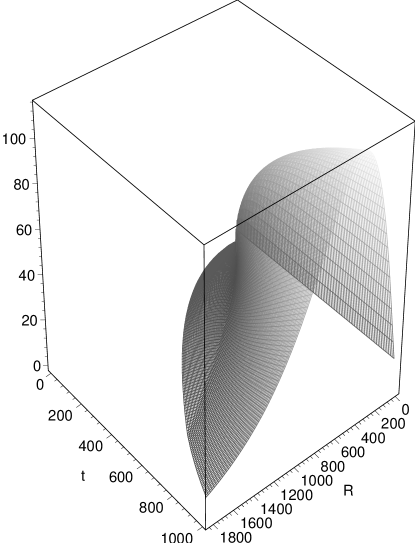
Figure 2: The ratio $\alpha_{2}$ in the entropy flux condition (42), for $\alpha=-\sqrt{3}/2$.

Despite the violations of these conditions, computing the entropy integral, outlined below, shows that (i) no counter-example of the Bousso bound(7) appears for all the cases considered, (ii) violations of the generalised bound (8) occur in a band region surrounding the apparent horizon surface, and (iii) the generalized bound holds in regions where $s^{a}k_{a}\neq 0$. These results indicate that neither the second nor third set of conditions are necessary for the validity of the Bousso bound (7).

The integral for the entropy on the light sheet is

$$S_{L}=\int_{L}s_{L}l^{a}\epsilon_{abcd}$$ (45)

where

$$\epsilon_{abcd} = \sqrt{-g}\ dt\wedge dr\wedge d\theta\wedge d\phi$$ (46)

$$= t^{2}r^{2}f^{(1-a)/a}{\rm sin}\theta\ dt\wedge dr\wedge d\theta\wedge d\phi.$$

With $l^{a}$ given by (22)

$$l^{a}\epsilon_{abcd} = t^{2}r^{2}(1-2/r)^{1-a}\ {\rm sin}\theta\ dr\wedge d\theta\wedge d\phi$$ (47)

$$-t^{2}r^{2}(1-2/r)\ {\rm sin}\theta\ dt\wedge d\theta\wedge d\phi$$

The integral is therefore

$$S_{L} = 2\pi\int_{r_{0}}^{r_{1}}r^{2}t(r)^{2}(1-2/r)^{1-a}s(t(r),r)\ dr$$ (48)

$$-2\pi\int_{t_{0}}^{t_{1}}r(t)^{2}t^{2}(1-2/r(t))\ s(t,r(t))\ dt$$

$$= 4\pi\int_{r_{0}}^{r_{1}}r^{2}t(r)^{2}(1-2/r)^{1-a}s(t(r),r)\ dr$$

for null geodesics $r(t)$ ( or $t(r))$ starting at coodinates $(t_{0},r_{0})$ and ending at $(t_{1},r_{1})$. The change in the area of the corresponding 2-spheres is

$$A(t,r)=4\pi tr^{2}\ (1-2/r)^{1-a}.$$ (49)

IV Results and Discussion

A selection of numerical results for entropy on light sheets appear in Tables 1 and 2. These were computed using integration routines in MAPLE in two stages. The first is the numerical integration to obtain the null geodesics $r(t)$ or $t(r)$, and the second uses this as input to compute the entropy integrals for a selection of starting times and radii $(t_{i},r_{i})$.

Table 1: This table shows the coordinates $(t,r,R)$ for spherical surfaces $B$ and $B^{\prime}$, the initial expansion $\theta_{i}$ on $B$, the area difference, and the computed light sheet entropy $S_{L}$. The first two rows verify the Bousso bound ($R_{f}=0$) for a small and a large sheet. The last two rows concern the generalized bound: the third row shows its validity for a small sheet, and the last row shows a violation for a large sheet with initial expansion $|\theta_{i}|<<1$. All numbers are for $\alpha=-\sqrt{3}/2$.

$(t_{i},r_{i},R_{i})$	$(t_{f},r_{f},R_{f})$	$\theta_{i}$	$\Delta A/4$	$S_{L}$
(1,5,3.10)	(2.31,2,0)	-6.3 $10^{-3}$	30.28	20.88
(15,30,108.95)	(38.16,2,0)	-5.5 $10^{-4}$	37288.21	21971.84
(30,30,154.07)	(30.09,29.9,153.77)	-1.3 $10^{-3}$	296.88	233.02
(14,31.5,110.86)	(28.32,16,75.17)	-1.7 $10^{-6}$	20861	22595

The main features of the results are the following: (i) The Bousso bound holds for all cases considered, (ii) the generalized bound is violated in cases where the magnitude of the initial expansion $\theta_{i}$ is sufficiently small, and (iii) the generalized bound holds for very small light sheets if $|\theta_{i}|$ is sufficiently large. Thus violations of this bound occur only in a band region around the apparent horizon surface.

Table 2: Similar data as for Table (1), but for $\alpha=\sqrt{3}/2$. These results are for the generalized bound where $R_{f}\neq 0$. The first row shows a violation of this bound for a large light sheet, where the initial expansion $|\theta_{i}|<<1$ on $B$. The second row shows that if this sheet is extended further, the bound begins to hold. The latter two rows show its validity for a small and a large sheet; for these cases $|\theta_{i}|$ is larger.

$(t_{i},r_{i},R_{i})$	$(t_{f},r_{f},R_{f})$	$\theta_{i}$	$\Delta A/4$	$S_{L}$
(16,30,119.44)	(32.32,15,84.46)	-4.0 $10^{-5}$	22411.07	25122
(16,30,119.44)	(38.15,10,60.85)	-4.0 $10^{-5}$	33190.46	27516
(40,30,188.86)	(40.1,29.9,188.47)	-1.0 $10^{-3}$	453.93	282
(40,30,188.86)	(72.6,3,23.74)	-1.0 $10^{-3}$	110284	26606

The basic intuition behind the covariant bounds is that entropy focusses light because entropy goes where matter goes. Therefore a large entropy density is associated with a smaller light sheet, and vice versa. Thus covariant entropy bounds are expected to hold even in regions of high energy density because this is compensated by the light sheets having smaller extents.

The violations of the generalized bound we find occur in regions of rather small $|\theta_{i}|$, which means that matter and entropy density are very low. It is therefore useful to see how the length scale $L\sim\rho^{-1/4}$ associated with the local energy density $\rho$ compares with the characteristic scale $\Delta R=R_{f}-R_{i}$ of the light sheet for the results in Tables 1 and 2. The intuition is that if $L<\Delta R$, then the characterization of entropy flows by the flux vector $s^{a}$ is a good approximation, and it is meaningful to compute entropy using the integral (39). (This issue has been discussed recently in bfm .)

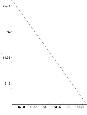
Figure 3: Plot of $L(R)=\rho(R)^{-1/4}$ for the light sheet in the third row of Table 1. The generalized bound holds for this small sheet even though $L>\Delta R(=0.3)$.

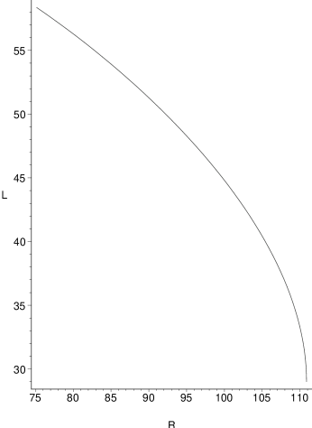
Figure 4: Plot of $L(R)=\rho(R)^{-1/4}$ for the light sheet in the forth row of Table 1. The generalized bound does not hold for this large ($\Delta R=35.7$) sheet.

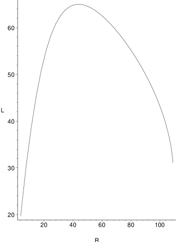
Figure 5: Plot of $L(R)=\rho(R)^{-1/4}$ for the light sheet in the second row of Table 1. The Bousso bound holds for this sheet (as it does for all cases considered).

Figures 3 and 4 show this variation respectively for the light sheets in rows three and four of Table 1. It is apparent from these figures that $L>\Delta R$ for both cases. For comparison, Figure 5 shows this variation for the second row of Table 1, which is a positive check of the Bousso bound. Here it is clear that the largest value of $L$ $(\sim 60)$ is less than $\Delta R$ $(\sim 110)$. Thus it is clear that this simple test is inconclusive as a means for eliminating counterexamples in inhomogeneous spacetimes, although it appears to work in an homogeneous spacetime bfm .

V Summary

We studied the covariant entropy bounds (7) and (8) in an inhomogeneous and time dependent scalar field spacetime. By explicit computation of entropy on light sheets, we find that the Bousso bound (7) holds in every case considered, and that the generalised bound (8) is violated if the expansion on the initial surface is sufficiently small.

The following conclusions may be drawn from these results: (i) The second set of sufficient conditions for the Bousso bound are violated for the spacetime we consider, due to violation of the sum condition (43). Nevertheless, the Bousso bound holds. This means that this set of conditions is not necessary. (ii) The violation of the generalized bound is not unambiguously attributable to the breakdown of the description of entropy by a local flux vector, since we have seen that this bound holds for small sheets where the characteristic wavelength of matter as measured by $\rho^{-1/4}$ is significantly larger than the extent $R_{f}-R_{i}$ of the light sheet. The flux condition (42), which is closely connected with the length scales argument used above fmw , also appears not to be a necessary condition for the generalized bound due to the example in Figure 3. Thus our results suggest that it is useful to determine what are the necessary conditions for both the Bousso and generalized bounds.

Since the very formulation of the covariant bounds requires a classical spacetime, the extent to which it gives insight into quantum gravity is rather limited. It would be of interest to see to what extent entropy bound formulations may be written down in quantum regimes where issues such as singularity avoidance can be addressed simultaneously. Our results indicate that it is not the singularities that threaten the bounds but rather the regions near the fairly classical apparent horizon surface, where there are violations of the generalised bound.

Acknowledgements I thank Don Marolf for comments. This work was supported by the Natural Science and Engineering Research Council of Canada.

References

- (1) J. D. Bekenstein, Generalized second law of thermodynamics in black hole physics, Phys. Rev. D 9, 3292 (1974); A universal upper bound on the entropy to energy ratio for bounded systems, Phys. Rev. D 23, 287 (1981).
- (2) G. t’Hooft, Dimensional reduction in quantum gravity, gr-qc/9310026.
- (3) L. Susskind, The world as a hologram, J. Math. Phys. 36 6377 (1995); hep-th/9409089.
- (4) R. Bousso, The Holographic Principle, Rev. Mod. Phys. 74, 825 (2002); hep-th/9906022.
- (5) W. Fischler and L. Susskind, Holography and cosmology hep-th/9806039.
- (6) R. Bousso, A covariant entropy conjecture, JHEP 07 004, (1999); hep-th/9905177.
- (7) E. Flanagan, D. Marolf, and R. Wald, Proof of classical versions of the Bousso entropy bound and of the Generalized Second Law, Phys. Rev. D 62 084035 (2000); hep-th/9908070.
- (8) V. Husain, E. Martinez and D. Nunez, Exact solution for scalar field collapse, Phys. Rev. D 50 (1994).
- (9) S. Hayward, The general laws of black hole dynamics, Phys. Rev. D 49, 6467 (1994); gr-qc/9303006.
- (10) R. Bousso, E. Flanagan, and D. Marolf, Simple sufficient conditions for the generalized covariant bound, hep-th/0305149.
- (11) R. C. Tolman, Relativity, thermodynamics and cosmology, (The Clarendon press, Oxford, 1934).
- (12) S. Das and V. Husain, AdS black holes, perfect fluids, and holography, hep-th/0303089.