Extended Lifetime in Computational Evolution of Isolated Black Holes

Abstract

Solving the 4-d Einstein equations as evolution in time requires solving equations of two types: the four elliptic initial data (constraint) equations, followed by the six second order evolution equations. Analytically the constraint equations remain solved under the action of the evolution, and one approach is to simply monitor them (unconstrained evolution).

The problem of the 3-d computational simulation of even a single isolated vacuum black hole has proven to be remarkably difficult. Recently, we have become aware of two publications that describe very long term evolution, at least for single isolated black holes. An essential feature in each of these results is constraint subtraction. Additionally, each of these approaches is based on what we call “modern,” hyperbolic formulations of the Einstein equations. It is generally assumed, based on computational experience, that the use of such modern formulations is essential for long-term black hole stability. We report here on comparable lifetime results based on the much simpler (“traditional”) $\dot{g}$ - $\dot{K}$ formulation.

With specific subtraction of constraints, with a simple analytic gauge, with very simple boundary conditions, and for moderately large domains with moderately fine resolution, we find computational evolutions of isolated nonspinning black holes for times exceeding $1000GM/c^{2}$.

We have also carried out a series of constrained 3-d evolutions of single isolated black holes. We find that constraint solution can produce substantially stabilized long-term single hole evolutions. However, we have found that for large domains, neither constraint-subtracted nor constrained $\dot{g}$ - $\dot{K}$ evolutions carried out in Cartesian coordinates admit arbitrarily long-lived simulations. The failure appears to arise from features at the inner excision boundary; the behavior does generally improve with resolution.

I Introduction

Binary black hole systems are expected to be the strongest possible astrophysical gravitational wave sources. In the final moments of stellar mass black hole inspiral, the radiation will be detectable in the current (LIGO-class) detectors. If the total binary mass is of the order of $10M_{\odot}$, the moment of final plunge to coalescence will emit a signal detectable by the current generation of detectors from very distant (Gpc) sources. The merger of supermassive black holes in the center of galaxies will be the dominant signal in the spaceborne LISA detector, and detectable out to large redshift.

Simulation of these mergers will play an important part in the prediction, detection, and the analysis of their gravitational signals in gravitational wave detectors. To do so requires a correct formalism which does not generate spurious singularities during the attempted simulation. Recent important workschKidteuk yo has been done in extending the computational lifetime of single isolated black hole simulations. We report here on such an extension which demonstrates that constraint subtraction by itself is adequate to produce very long-lived simulations. We demonstrate this even for a very simple (“traditional”) $\dot{g}$ - $\dot{K}$ formulation, with specific subtraction of constraints (which are analytically zero) for single isolated nonspinning black holes, with a simple analytic gauge (lapse and shift not “densitized”; see IV.1 below), with very simple boundary conditions, and for moderately large domains with moderately fine resolution.

We have also found that constrained 3-d evolution with densitized lapse can produce substantially stabilized long-term single holes, even for subtractions that differ from the values that we have found to be optimal in the unconstrained case, and we give some preliminary constrained evolution results.

However, in all cases we find that attempting to carry out the simulations on very large domains ($\pm 20M$, or larger) still yields eventually unstable simulations, by any of the methods reported here.

II $3+1$ Formulation of Einstein Equations

We take a Cauchy formulation (3+1) of the ADM type, after Arnowitt, Deser, and Misner ADM . In such a method the 3-metric $g_{ij}$ and its momentum $K_{ij}$ are specified at one initial time on a spacelike hypersurface, and evolved into the future. The ADM metric is

$${\rm d}s^{2}=-(\alpha^{2}-\beta_{i}\beta^{i})\,{\rm d}t^{2}+2\beta_{i}\,{\rm d}t\,{\rm d}x^{i}+g_{ij}\,{\rm d}x^{i}\,{\rm d}x^{j}$$ (1)

where $\alpha$ is the lapse function and $\beta^{i}$ is the shift 3-vector; these gauge functions encode the coordinatization.†

The Einstein field equations contain both hyperbolic evolution equations and elliptic constraint equations. The constraint equations for vacuum in the ADM decomposition are:

$$H=\frac{1}{2}[R-K_{ij}K^{ij}+K^{2}] = 0,$$ (2)

$$H^{i}=\nabla_{j}\left(K^{ij}-g^{ij}K\right) = 0.$$ (3)

Here $R$ is the 3-d Ricci scalar constructed from the 3-metric, and $\nabla_{j}$ is the 3-d covariant derivative compatible with $g_{ij}$. Initial data must satisfy these constraint equations; one may not freely specify all components of $g_{ij}$ and $K_{ij}$.

In this paper we are concerned only with single isolated black holes. From this point of view the problem is not solving the initial value equations, since the data are known analytically. Instead, the question is one of the stability of the solution as these data are evolved computationally. The evolution equations from the Einstein system are

$$\dot{g}_{ij}=-2\alpha K_{ij}+\nabla_{j}\beta_{i}+\nabla_{i}\beta_{j}$$ (4)

and

$$\dot{K}_{ij}=-\nabla_{i}\nabla_{j}\alpha+\alpha(R_{ij}-2K_{ik}K^{k}_{~{}j}+KK_{ij})+\beta^{k}\nabla_{k}K_{ij}+K_{ik}\nabla_{j}\beta^{k}+K_{jk}\nabla_{i}\beta^{k}$$ (5)

where a dot ( $\dot{}$ ) denotes the partial derivative with respect to time, and $R_{ij}$ is the 3-d Ricci tensor.

We call this form of the Einstein equations of ADM type, referring to the fundamental development ADM ; this specific form is called the $\dot{g}$ - $\dot{K}$ form. Here, Eq. (2)–Eq. (3), the constraint equations, are the vacuum Einstein equations ${}^{4}G_{00}=0$ and ${}^{4}G_{0i}=0$ respectively. Eq. (4)–Eq. (5), the evolution equations, are a first order form of the vacuum Einstein equations ${}^{4}R_{ij}=0$.

The true ADM form writes the evolution equations as ${}^{4}G_{ij}=0$, the space components of the 4-d Einstein tensor, rather than the Ricci tensor. Frittelli and Reula49Frittelli have shown that with certain (rather strong) assumptions, there is stable maintenance of the constraints under unconstrained evolution for Eq. (4)–Eq. (5), but only neutral stability for ${}^{4}G_{ij}=0$.

III Data Form

In this paper we consider only single isolated black holes, so the data setting problem is already solved; we use Kerr-Schild data, which describes a single isolated spinning or nonspinning black hole hole.

The Kerr-Schild KerrSchild form of a black hole solution describes the spacetime of a single black hole with mass, $m$, and specific angular momentum, $a=j/m$, in a coordinate system that is well behaved at the horizon:

$${\rm d}s^{2}=\eta_{\mu\nu}\,{\rm d}x^{\mu}\,{\rm d}x^{\nu}+2H_{KS}(x^{\alpha})l_{\mu}l_{\nu}\,{\rm d}x^{\mu}\,{\rm d}x^{\nu},$$ (6)

where $\eta_{\mu\nu}$ is the metric of flat space, $H_{KS}$ is a scalar function of $x^{\mu}$, and $l_{\mu}$ is an (ingoing) null vector, null with respect to both the background and the full metric,

$$\eta^{\mu\nu}l_{\mu}l_{\nu}=g^{\mu\nu}l_{\mu}l_{\nu}=0.$$ (7)

Comparing the Kerr-Schild metric with the ADM decomposition Eq. (1), we find that the $t=\hbox{\rm constant}$ 3-space metric is: $g_{ij}=\delta_{ij}+2H_{KS}l_{i}l_{j}$. Further, the ADM gauge variables are

$$\beta_{i}=2H_{KS}l_{0}l_{i},$$ (8)

and

$$\alpha=\frac{1}{\sqrt{1+2H_{KS}l_{0}^{2}}}.$$ (9)

The extrinsic curvature can be computed from Eq.(4):

$$K_{ij}=\frac{1}{2\alpha}[\nabla_{j}\beta_{i}+\nabla_{i}\beta_{j}-\dot{g}_{ij}],$$ (10)

Each term on the right hand side of this equation is known analytically; in particular, for a black hole at rest, $\dot{g}_{ij}=0$.

The general non-moving black hole metric in Kerr-Schild form (written in Kerr’s original rectangular coordinates) has

$$H_{KS}=\frac{mr}{r^{2}+a^{2}\cos^{2}\theta},$$ (11)

and

$$l_{\mu}=\left(1,\frac{rx+ay}{r^{2}+a^{2}},\frac{ry-ax}{r^{2}+a^{2}},\frac{z}{r}\right),$$ (12)

where $r,~{}\theta$ (and $\phi$) are auxiliary spheroidal coordinates, $z=r(x,y,z)\cos\theta$, and $\phi$ is the axial angle. $r(x,y,z)$ is obtained from the relation,

$$\frac{x^{2}+y^{2}}{r^{2}+a^{2}}+\frac{z^{2}}{r^{2}}=1,$$ (13)

giving

$$r^{2}=\frac{1}{2}(\rho^{2}-a^{2})+\sqrt{\frac{1}{4}(\rho^{2}-a^{2})^{2}+a^{2}z^{2}},$$ (14)

with

$$\rho=\sqrt{x^{2}+y^{2}+z^{2}}.$$ (15)

In the nonspinning case, one has $l_{i}=x_{i}/r$, so that $\alpha=\frac{1}{\sqrt{1+2m/r}}$, and $\beta_{i}=2mx_{i}/r$.

IV Constraint Subtraction

The difference between Eq. (4)–Eq. (5), and ${}^{4}G_{ij}=0$, is a specific subtraction of the constraint equations. This has led to the consideration by a number of groups, of constraint subtraction with coefficients chosen by numerical search, or by analytical estimate (perhaps combined with numerical search) to improve the long-term stability of the unconstrained evolution. We have carried out such a numerical search, and we use the following constraint subtraction:

$$-\alpha H(0.464\,g_{i\,j}\,+0.36\ K_{i\,j}\,)$$ (16)

on the right hand side of the $\dot{K}_{ij}$ equation (Eq. (5)). We have found that this subtraction substantially improves the unconstrained evolution of nonspinning single-hole data. For these evolutions we choose fixed (Dirichlet) outer boundary conditions set equal to the analytical value. In every case the simulation excises the interior of the black hole. One-sided differencing is used near the inner (mask) boundary, so no boundary condition is needed there, consistent with the property of the horizon as a causal boundary. The mask is specified at a radius of 0.75 M. The solution employs the SUNDIALS package for time integration SUNDIALS ; CVODES . The spatial discretization is fourth order, and the time evolution is typically fourth order (variable-order according to the relative and absolute error tolerances). This approach successfully stabilizes the evolutions for domains of $\pm 10M$, as shown in Figure 1. For larger domains, however, the system is increasingly shorter lived, as shown in Figure 2. As a simple measure of the quality of solution, we present the either the $l_{2}$ norm or rms norm of the Hamiltonian constraint constructed via a straightforward fourth order differencing scheme from the code results.

Although it is difficult to compare subtraction techniques across different formal representations of the Einstein equations, we do find typically much smaller coefficients of subtraction (of order $0.5$) than found for different formulations, e.g. schKidteuk with a constraint subtraction of order $-12.$ The BSSN formulation of yo is also substantially different from ours (there is a subtraction from the $\dot{g}_{ij}$ equation, for instance, which we do not have, and the subtraction from the $\dot{K}_{ij}$ equation is different from ours), though the coefficient of subtraction from $\dot{K}_{ij}$ for this approach is small, comparable to ours.

IV.1 Densitized Lapse

There is extensive evidence in the literature that a densitized lapse improves the hyperbolicitygr-qc/0402123 of the (at best) weakly hyperbolic ADM form of the Einstein equations. We implement densitized lapse for single black hole simulations by writing

$$\alpha=\alpha_{\rm analytic}(g/g_{\rm analytic})^{p},$$ (17)

where $\alpha_{\rm analytic}$ is the explicit lapse as a function of coordinates given by Eq. (9), $g_{\rm analytic}$ is the analytic Kerr-Schild $3-$metric determinant as a function of coordinates, ($g_{\rm analytic}=1+2Hl_{t}^{2}$, gr-qc/0002076 ), $g$ is the computational $3-$metric determinant, and $p$ is an adjustable positive constant usually taken to be $\frac{1}{3}$ or $\frac{1}{2}$. In fact we find that densitized lapse does not enhance constraint-subtracted lifetime, though it does contribute substantially to longer lifetime in constrained evolutions described below.

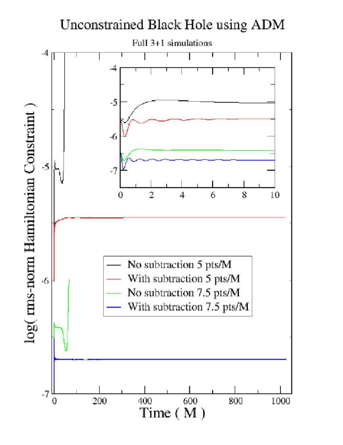
Figure 1: The log of the rms norm of the Hamiltonian constraint violations for constraint-subtracted and unsubtracted nonspinning black hole simulations with excision. The simulations were performed at resolutions of $M/5$ and $M/7.5$ on a domain size of $\pm 10M$. The long-lived runs employed optimal constraint subtraction (Eq. (16)). The short-lived run employed no subtraction.

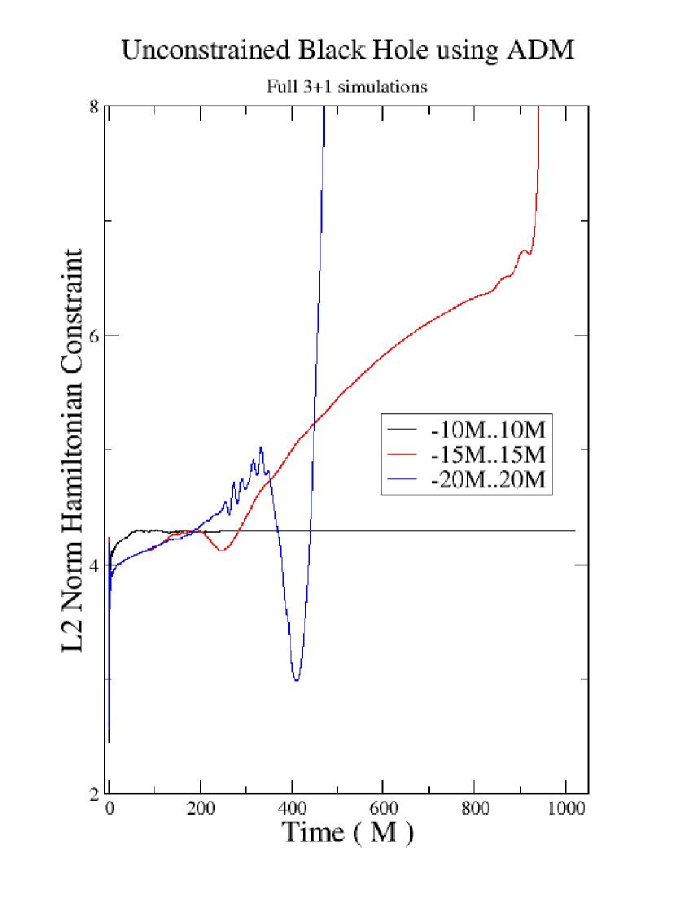
Figure 2: The $l_{2}$ norm of the Hamiltonian constraint violation for constraint-subtracted and unsubtracted nonspinning black hole simulations with excision performed at a resolution of $M/5$ on a domain sizes of $\pm 10M$, $\pm 15M$, or $\pm 20M$. All cases employed the optimal constraint subtraction (Eq. (16)). As the computational domain size increases, the simulation is increasingly shorter lived.

V Constrained Evolution

The evolution of Kerr-Schild data must continue to satisfy the constraint equations, Eqs. (2)–(3) as we evolve away from the initial data. However, if we choose nonoptimal (e.g. zero) constraint subtraction for even nonspinning black holes, the evolution leads to an eventual violation of the constraints. Hence we have investigated constrained evolution, solving the constraint equations as part of the time update of the evolution equations.

The postevaluated tracking of constraint errors [residual postevaluation] shown in Figures 1–2 used the direct discretization of the constraint equations Eq. (2) and Eq. (3). For constrained evolution we need instead to implement an accurate, efficient method of constraint solution. We adopt the conformal transverse-traceless method of York and collaborators YP -Bowen+York which consists of a conformal decomposition with a scalar $\phi$ that adjusts the metric, and a vector potential $w^{i}$ that adjusts the longitudinal components of the extrinsic curvature. The constraint equations are then solved for these new quantities $\phi$, $w^{i}$ such that the complete solution fully satisfies the constraints.

Applying this approach to constrained evolution, the metric and traceless extrinsic curvature in the middle of a timestep (after an explicit integration forward in time) are taken as conformal trial functions $\tilde{g}_{ij}$ and $\tilde{A}^{ij}$.

The physical metric at the end of the full timestep (i.e. after the constraint equation solve), $g_{ij}$, and the trace-free part of the extrinsic curvature at the end of the full timestep, $A_{ij}$, are related to the background fields through a conformal factor:

$$g_{ij} = \phi^{4}\tilde{g}_{ij},$$ (18)

$$A^{ij} = \phi^{-10}(\tilde{A}^{ij}+\tilde{(lw)}^{ij}).$$ (19)

Here $\phi$ is the conformal factor, and $\tilde{(lw)}^{ij}$ will be used to cancel any possible longitudinal contribution. $w^{i}$ is a vector potential, and

$$\tilde{(lw)}^{ij}\equiv\tilde{\nabla}^{i}w^{j}+\tilde{\nabla}^{j}w^{i}-\frac{2}{3}\tilde{g}^{ij}\tilde{\nabla_{k}}w^{k}.$$ (20)

The trace $K$ is not corrected:

$$K=\tilde{K}.$$ (21)

Writing the Hamiltonian and momentum constraint equations in terms of the quantities in Eqs. (18)–(21), we obtain four coupled elliptic equations for the fields $\phi$ and $w^{i}$ YP :

$$\tilde{\nabla}^{2}\phi = \left(1/8\right)\left[\tilde{R}\phi\right.+\frac{2}{3}\tilde{K}^{2}\phi^{5}-$$ (22)

$$\phi^{-7}\left(\tilde{A}{{}^{ij}}+(\tilde{lw})^{ij}\right)\left.\left(\tilde{A}_{ij}+(\tilde{lw})_{ij}\right)\right],$$

$$\tilde{\nabla}_{j}(\tilde{lw})^{ij} = \frac{2}{3}\tilde{g}^{ij}\phi^{6}\tilde{\nabla}_{j}\tilde{K}-\tilde{\nabla}_{j}\tilde{A}{{}^{ij}}.$$ (23)

These equations are solved to complete each time-update step. The resulting solved $g_{ij}$ and $K_{ij}$ are taken as the data for the next time-update. Notice that these equations require no specific gauge choice. A similar approach also can be applied to other formulations which generally have a larger number of constraints.

V.1 Elliptic Equation Boundary Conditions

A solution of the elliptic constraint equations requires that boundary data be specified on both the outer boundary and on the surfaces of any masked regions. For the elliptic solution here we can choose simple conditions, $\phi=1$ and $w^{i}=0$, on the masked region surrounding the singularity. Because we solve the problem on a finite domain, we also must provide an outer boundary condition for $\phi$ and $w^{i}$. For this demonstration of the technique, we choose the same conditions at the outer boundary of the domain: $\phi=1$ and $w^{i}=0$. In long term evolution we expect the evolved solution to converge (as the solution is refined) to a solution of the constraints, so a global solution $\phi=1$ and $w^{i}=0$ is expected in this analytic limit. For achievable resolutions, however, the quantities $\phi$ and $w^{i}$ deviate from this prediction.

VI Constrained Evolution Results

The elliptic constraint equations are solved either by a PETSc PETSC_1 ; PETSC_2 ; PETSC_3 GMRES solver or KINSOL SUNDIALS GMRES solver; the spatial differencing is fourth order. We present below (Figures 3 - 6) the results of preliminary constrained evolution of nonspinning black holes. Figure 3 shows the rms norm of Hamiltonian and momentum constraints for these simulations. Compared to the relatively short term crash of the unconstrained evolution, the constrained evolution clearly does stabilize single black hole evolutions in small domains, regardless of the precise subtraction. To fully understand the content of Figure 3, consider that, even if the residual limit in the solution of the constraint equations, Eq. (22) – Eq. (23), is set to extremely small values (it can be set very near to machine precision, meaning that the discretized matrix form of equations Eq. (22) – Eq. (23) can be solved to fractional errors of order $10^{-15}$), the post-evaluations of the constraint residuals will typically show the expected $zero$ only to the internal discretization accuracy (here fourth order). This is why the constrained solution shown in Figure 3 shows a finite (but convergent) level of Hamiltonian constraint violation.

Figures 4-6 show a constrained $\dot{g}-\dot{K}$ evolution with densitized lapse, at three resolutions ($M/5,M/7.5,M/10$). The $M/5$ evolution became unstable before $t=100M$. The $M/7.5$ run began showing large residuals at $t\approx 350M$. The $M/10$ run shows better behavior than $M/7.5$, at least initially It shows a similar late time instability which tracks (at smaller error) the behavior of the $M/7.5$ case, but around $150M$ ceases to be convergent; see Figure 5. Figure 6 shows the 2d $z=0$ behavior of the residual component $G_{xx}$ at $t=100M$. The “red-blue” pattern of the features near the excision mask indicate that most of the error develops there. The residual becomes more asymmetrical at later times.

VII CORRECTNESS OF CONSTRAINED EVOLUTION

The constraint maintenance approach uses what has been called in magnetohydrodynamics, a projection methodprojection . This method for constrained evolution raises questions about the meaning of the solutions obtained. This is sometimes put bluntly: “Accepting that the method finds solutions of the full Einstein system, how do we know that the found solution is the right one?” By this is meant that the constraint solution step may somehow move the solution back to an “erroneous” point on the space of constraint solutions. For instance, it might be possible that although the evolution substep and the constraint substep are individually convergent computational processes, the result of combining them is in some manner not convergent. (In the much simpler MHD case there are analytical proofs that projection minimizes the resultant error in the magnetic field, in a convergent way.projection )

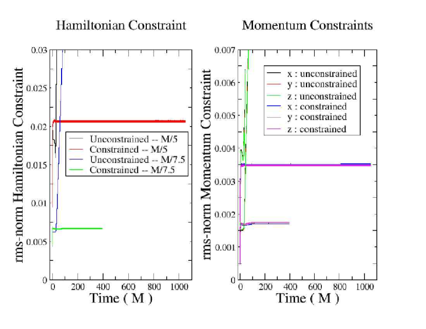
Figure 3: The rms norm of the Hamiltonian and momentum constraints for simulations of a Schwarzschild (nonspinning) black hole with excision. None of the simulations used any constraint subtraction. The simulations were performed at resolutions of either $M/5$ or $M/7.5$ on a domain size of $\pm 5M$. The long-lived runs employed constrained evolution as described in the text. The short-lived runs were unconstrained.

There are several parts to the response. (It will be clear that we do not pretend to a rigorous analytical proof.) To begin with, we have constructed completely independent “residual evaluators” for the full Einstein systemchoptuikSB . These evaluate the Einstein tensor, working just from the metric produced by the computational solution. They are completely different from the way the equations are expressed in the constrained evolution code. As we show in Figures 4,5, the resulting residual is in every case initially small (order of truncation error) and convergent. Thus we have achieved a computational solution to the Einstein system. Note that our full Einstein equation residual evaluator checks both the constraints (Einstein equations at one time), and the evolution equations connecting different time steps.

The residual evaluators are written to return fourth order accurate results. Since they have now been verified and show convergence of the solution, we appeal to the assumption that the Einstein system is not singular at the solution manifold. Thus we expect that the computational result converges to the analytical solution of the Einstein equations. We have converged to a spacetime configuration. Physical consistency and generality imply that it is the physically unique one that contains the initial data slice. We also note that, as in the situation in Figure 5, the convergence is eventually lost in some simulations; these simulations are no longer solving Einstein’s equations.

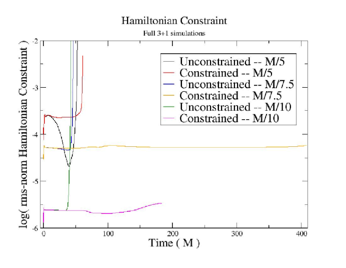
Figure 4: The log of the rms norm for the Hamiltonian constraint in simulations evolving a nonrotating Kerr-Schild black hole with a spatial domain of [$-10M...10M$] at three resolutions: $M/5,M/7.5,$ and $M/10.$ The excision radius was $0.5M$ in all constrained and unconstrained cases. All simulations used a densitized lapse with $p=\frac{1}{3}$. The constraints were solved in the constrained evolution cases every $0.05M$ everywhere on the domain except those points where $r<2.0M$. Independent residual evaluations for the constrained cases with resolution M/7.5 and M/10 are found in Figure 5

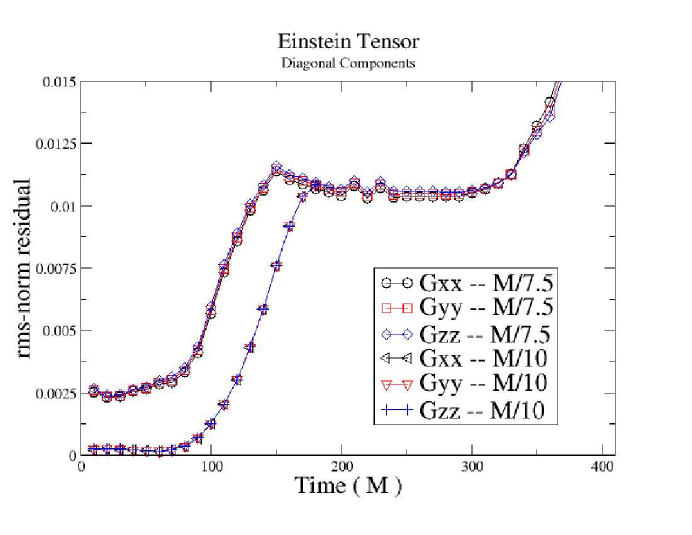
Figure 5: The rms norm of the diagonal spatial components of the Einstein tensor for the M/7.5 and M/10 constrained simulations presented in Figure 4

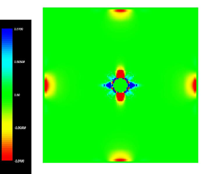
Figure 6: The z = 0 plane of the Einstein tensor component $G_{xx}$ at time $100M$ for the $M/7.5$ constrained evolution presented in Figures 4, 5.

It is of interest to ask why our approach has not been implemented previously. A number of factors were at work. It has been universally assumed that the computational overhead of elliptic solvers is excessive. Choptuik ChoptuikPC indicates a time penalty of $\times 2$, incurred by a fully constrained $2d$ evolution, compared to free evolution. This cost is justified by the much longer physical lifetimes achieved in the ($2d$) evolutions of Ref gr-qc0301006 ; Choptuik’s factor of two in time is considered a small penalty. However, in previous implementations of constrained ($2d$) evolution, one additionally had the problem that the solvers were restricted, for instance to conformally flat situations. This required strong gauge constraints on the evolution, and meant that generally one re-solved a strongly nonlinear equation (comparable to the initial value problem), on each time step. But we have found, even working with straightforward package solvers, that the penalty for our approach is only of order 30%. This is because our constraint solver (developed for Kerr-Schild superposed initial data), is in fact completely general with no form restrictions on the background. (There are, of course, general conditions on the elliptic equations to allow their solution restrictions , but we have encountered no difficulties in working with physically realistic configurations).

Thus our elliptic solver can use backgrounds that are strongly nonflat. They may be strongly nonflat, but they are already very close to constraint solution. This is so because they arise from evolving one timestep with an accurate time integrator; we use a package integrator which is typically fourth order accurate in time, and the spatial discretization is also fourth order. There is thus only a very small correction arising from the elliptic solve, and minimal outer iteration is required. Further, we take note of the fact that our explicit time integration has a certain inherent order of truncation error. Thus we do not in fact set the residual limit for the elliptic solve anywhere near machine accuracy. Instead we set it so that it produces errors which are consistent in size with the evolution truncation error. This reduces the internal iteration in the solver to a very small number. Finally, computational resources are now becoming adequate for constrained 3-d evolution. $1$Tflop/sec Computers are now accessible, making this work plausible. It will always be the case that constrained evolution is more computation- and memory- intensive than unconstrained, but the time has arrived that interesting constrained evolutions are possible. Further, ongoing computational infrastructure improvements will make this level of computation generally accessible. Well within a decade, desktop access to $10$ Tflop/sec will mean that constrained evolutions at LISA- or LIGO- relevant resolutions will become unexceptional.

VIII Discussion

We have demonstrated that the analytical formulation is not critical to long term evolution of single black holes, if the correct constraint subtraction is used. Thus, “modern” approaches that pose explicitly hyperbolic approaches are not essential; “traditional” $\dot{g}$ - $\dot{K}$ methods produce comparably long evolutions. The evidence seems to be that there are many formulations and subtraction schemes that lead to long-term single black hole stability; we have found an especially simple one.

However, we have found, consistent with theoretical estimates, that the precise subtraction is critical (a fraction to two or three decimals). To attack this problem, we have carried out periodic solution of the elliptic constraint equations as part of the time integration, to enable fully constrained evolutions of the Einstein equations. Our initial results demonstrate dramatic improvement of long term stability of a nonspinning black hole simulation. Because we solve the constraints, constraint subtraction is irrelevant in this case. We are beginning exploration of the constrained evolution approach in spacetimes involving single moving, and multiple interacting black holes. We find substantial improvement from constraint solving in every simulation, but we have not achieved infinite-lived $\dot{g}-\dot{K}$ simulations, even with densitized lapse (which is known to improve the hyperbolicity of the system of equations). We have begun an approach where the inner excision is made at a constant coordinate surface that coincides with the apparent horizon (essentially spherical, or spheroidal coordinates) near the excision regionmattDiss . This approach addresses concerns about the validity of the stair-step (LEGO) excision region (gr-qc/0302072 ). (Additionally the best long-lived isolated black hole simulation to date has been carried out by Ref schKidteuk with a pseudo-spectral method with apparent horizon conforming coordinates.)

Our approach uses coordinates which are spherical near the hole, with a cartesian region further away. It is hoped that this approach may exhibit some of the good properties and long lifetime of the codes described in schKidteuk .

References

- (1) Mark A. Scheel, Lawrence E. Kidder, Lee Lindblom, Harald P. Pfeiffer, Saul A. Teukolsky, “Toward stable 3D numerical evolutions of black-hole spacetimes,” Phys. Rev. D66 124005 (2002)[arXiv:gr-qc/0209115].
- (2) Hwei-Jang Yo, Thomas W. Baumgarte, Stuart L. Shapiro, “Improved numerical stability of stationary black hole evolution calculations,” Phys. Rev. D66 084026 (2002) [arXiv:gr-qc/0209066].
- (3) R. Arnowitt, S. Deser, and C. Misner in Witten, Gravitation, an Introduction to Current Research (Wiley, New York 1962).
- (4) Frittelli, S., and Reula, O., “First-order symmetric-hyperbolic Einstein equations with arbitrary fixed gauge”, Phys. Rev. Lett., 76, 4667-4670, (1996).
- (5) R. Kerr and A. Schild, “Some Algebraically Degenerate Solutions of Einstein’s Gravitational Field Equations,” in Applications of Nonlinear Partial Differential Equations in Mathematical Physics, Proc. of Symposia B Applied Math., Vol XVII (1965); “A New Class of Solutions of the Einstein Field Equations”, Atti del Congresso Sulla Relitivita Generale: Problemi Dell’Energia E Onde Gravitazionala G. Barbera, Ed. (1965).
- (6) A. Hindmarsh, R. Serban and C. Woodward, “SUNDIALS home page”, http://www.llnl.gov/CASC/sundials/ (2002).
- (7) A. Hindmarsh and R. Serban, “User Documentation for CVODES”, (Center for Applied Scientific Computer, Lawrence Livermore National Laboratory, 2002).
- (8) A. Taylor and A. Hindmarsh, “User Documentation for KINSOL, A Nonlinear Solver for Sequentail and Parallel Computers”, (Center for Applied Scientific Computer, Lawrence Livermore National Laboratory, 1998).
- (9) Gabriel Nagy, Omar E. Ortiz and Oscar A. Reula “Strongly hyperbolic second order Einstein’s evolution equations”, gr-qc/0402123 (2004).
- (10) J. York and T. Piran “The Initial Value Problem and Beyond”, Spacetime and Geometry: The Alfred Schild Lectures, R. Matzner and L. Shepley Eds. University of Texas Press, Austin, Texas. (1982); G. Cook, “Initial Data for the Two-Body Problem of General Relativity”, Ph.D. Dissertation, The University of North Carolina at Chapel Hill (1990).
- (11) N. Ó. Murchadha and J. W. York, Jr., Phys. Rev. D10, 428 (1974); N. Ó. Murchadha and J. W. York, Jr., Phys. Rev. D10, 437 (1974); N. Ó. Murchadha and J. W. York, Jr., Gen. Relativ. Gravit. 7 257 (1976).
- (12) J. W. York, Jr., Phys. Rev. Lett. 82, 1350 (1999).
- (13) J. R. Wilson and G. J. Mathews, Phys. Rev. Lett. 75, 4161 (1995); J. R. Wilson and G. J. Mathews, and P. Marronetti, Phys. Rev. D54, 1317 (1996)
- (14) J. Bowen and J. W. York, Phys. Rev. D21, 2047 (1980).
- (15) Mijan F. Huq, Matthew W. Choptuik and Richard A. Matzner, “Locating Boosted Kerr and Schwarzschild Apparent Horizons” Physical Review D66, 084024 (2002).
- (16) M. Choptuik, Personal communication.
- (17) S. Balay, K. Buschelman, W. D. Gropp, D. Kaushik, M. Knepley, L. C. McInnes, B. F. Smith and H. Zhang, “PETSc home page”, http://www.mcs.anl.gov/petsc (2001).
- (18) S. Balay, K. Buschelman, W. D. Gropp, D. Kaushik, M. Knepley, L. C. McInnes, B. F. Smith and H. Zhang, “PETSc Users Manual”, ANL-95/11 - Revision 2.1.5 (Argonne National Laboratoy, 2002).
- (19) S. Balay, K. Buschelman, W. D. Gropp, D. Kaushik, M. Knepley, L. C. McInnes, B. F. Smith and H. Zhang, “Efficient Management of Parallelism in Object Oriented Numerical Software Libraries”, Modern Software Tools in Scientific Computing, E. Arge, A. M. Bruaset, and H. P. Langtangen, editors, (Birkhauser Press, 1997), pp. 163-202.
- (20) Gioel Calabrese, Luis Lehner, David Neilsen, Jorge Pullin, Oscar Reula, Olivier Sarbach, Manuel Tiglio, “Novel finite-differencing techniques for numerical relativity: application to black hole excision”, Classical and Quantum Gravity 20 L245-L252 (2003).
- (21) G. Toth “The B Constraint in Shock-Capturing Magnetohydrodynamics Codes” Jour. Comp. Phys. 161 605 (2002).
- (22) Personal communication (2003).
- (23) M. W. Choptuik, E. W. Hirschmann, S. L. Liebling, and F. Pretorius, “An Axisymmetric Gravitational Collapse Code” Class. Quant. Grav. 20, 1857-1878 (2003).
- (24) Y. Choquet-Bruhat, J. Isenberg and J. W. York, Phys. Rev. D61 084034 2000
- (25) Matthew Anderson, “Constrained Evolution in Numerical Relativity” Ph.D. dissertation, The University of Texas at Austin (2004).