Formation of Schwarzschild black hole from the scalar field collapse in four-dimensions.

Abstract

We obtain a new self-similar solution to the Einstein’s equations in four-dimensions, representing the collapse of a spherically symmetric, minimally coupled, massless, scalar field. Depending on the value of certain parameters, this solution represents the formation of naked singularities and black holes. Since the black holes are identified as the Schwarzschild ones, one may naturally see how these black holes are produced as remnants of the scalar field collapse.

Since the first analytical model of gravitational collapse proposed, using general relativity [1], many works have been done in this area. An important model is the one where the collapsing matter is represented by a massless scalar field and the space-time has a spherical symmetry (Einstein-scalar model). D. Christodoulou has pioneered analytical studies of that model [2]. In particular, he showed that for a self-similar scalar field collapse there are initial conditions which result in the formation of black holes, naked singularities and bouncing solutions.

Many analytical results obtained by Christodoulou have been confirmed, by numerical studies of the Einstein-scalar model, by M. W. Choptuik [3]. Other authors have investigated the Einstein-scalar model numerically and analytically confirming the above results [4]. In particular, we may mention the works in references [5], [6]. There, the authors were able to reproduce qualitatively, in an analytical solution [7], the results derived numerically in [3].

The Roberts solution [7], has two arbitrary parameters $\alpha$ and $\beta$. In the work in reference [5], the author fixed $\beta=1$ and let $\alpha$ vary in the range $[1/4,-\infty]$. Once $\beta$ is fixed, $\alpha$ determines also the scalar field strength. It will be zero for $\alpha=1/4$ and it will increase for decreasing values of $\alpha$. The scalar field eventually diverges for $\alpha\to-\infty$. Starting with $\alpha=1/4$, the scalar field is zero and one has Minkowski space-time. Then, for $0<\alpha<1/4$, although the field is non-longer zero its strength is not enough to initiate the collapse. The space-time in this case represents a bouncing. For $\alpha=0$ the gravitational collapse begins and a naked singularity is formed at $r=0$. If one increases even further the field strength by letting $\alpha$ takes values in the range $-\infty<\alpha<0$, one has the black hole formation. Therefore, if one turns the scalar field on and gradually increases its strength one will see all the collapse stages described above. Suppose now, one decides to turn the scalar field off, which will eventually happen for one has a limited amount of energy. One will see all the collapse stages described above, in the reverse order. Starting with the black hole and finishing with the Minkowski space-time. So, we may conclude that the Roberts solution does not produce an eternal black hole that will be left as a remnant of the scalar field collapse. Once the scalar field is turned off one loses all trace of the collapse. It is not difficult to see that one may obtain the above result even if one let $\beta$ vary in an appropriate range.

One expects that the Schwarzschild black hole results from the collapse of a spherical symmetric neutral scalar field. So far, the only way to obtain this black hole as the result of the scalar field collapse was by joining an analytical solution to the Einstein-scalar equations that represents the collapse with the Vaidya solution [8]. Of course, this procedure generates the Schwarzschild black hole since it is a particular case of the Vaidya one. In reference [8], the authors joined the Roberts solution [7] with the exterior Vaidya solution.

In the present paper we would like to present a new solution to the Einstein’s equation representing the self-similar, spherically symmetric, collapse of a minimally coupled, neutral, massless, scalar field, in four-dimensions. As we shall see this solution has two parameters, in the same way as Roberts’ solution. Depending on the value of these parameters, we may have the formation of naked singularities and black holes. Since the black holes are identified as the Schwarzschild ones, we shall see how these black holes are produced as remnants of the scalar field collapse.

We shall start by writing down the ansatz for the space-time metric. As we have mentioned before, we would like to consider the spherically symmetric, self-similar, collapse of a massless scalar field in four-dimensions. Therefore, we shall write our metric ansatz as,

$$ds^{2}\,=\,-\,2e^{2\sigma(u,v)}dudv\,+\,r^{2}(u,v)d\Omega^{2}\,,$$ (1)

where $\sigma(u,v)$ and $r(u,v)$ are two arbitrary functions to be determined by the field equations, $(u,v)$ is a pair of null coordinates varying in the range $(-\infty,\infty)$, and $d\Omega^{2}$ is the line element of the unit sphere.

The scalar field $\Phi$ will be a function only of the two null coordinates and the expression for its stress-energy tensor $T_{\alpha\beta}$ is given by [9],

$$T_{\alpha\beta}\,=\,\Phi,_{\alpha}\Phi,_{\beta}\,-\,{1\over 2}g_{\alpha\beta}\Phi,_{\lambda}\Phi^{,_{\lambda}}\,.$$ (2)

where , denotes partial differentiation.

Now, combining Eqs. (1) and (2) we may obtain the Einstein’s equations which in the units of Ref. [9] and after re-scaling the scalar field, so that it absorbs the appropriate numerical factor, take the following form,

$$2(rr,_{uv}\,+\,r,_{u}r,_{v})\,+\,e^{2\sigma}\,=\,0\,,$$ (3)

$$2rr,_{vv}\,-\,4rr,_{v}\sigma,_{v}\,=\,-\,r^{2}(\Phi,_{v})^{2}\,,$$ (4)

$$2rr,_{uu}\,-\,4rr,_{u}\sigma,_{u}\,=\,-\,r^{2}(\Phi,_{u})^{2}\,,$$ (5)

$$2(r^{2}\sigma,_{uv}\,+\,rr,_{uv})\,=\,-\,r^{2}(\Phi,_{u}\Phi,_{v})\,,$$ (6)

The equation of motion for the scalar field, in these coordinates, is

$$r\Phi,_{uv}\,+\,r,_{u}\Phi,_{v}\,+\,r,_{v}\Phi,_{u}\,=\,0\,.$$ (7)

The above system of non-linear, second-order, coupled, partial differential equations (3)-(7) can be solved if we impose that it is continuously self-similar. More precisely, the solution assumes the existence of an homothetic Killing vector of the form,

$$\xi\,=\,u{\partial\over\partial u}\,+\,v{\partial\over\partial v}\,,$$ (8)

Following Coley [10], equation (8) characterizes a self-similarity of the first kind. We can express the solution in terms of the variable $z=v/u$.

In order to obtain our solution, we shall implement the self-similarity in the above equations (3-7) in a slightly different way than previous works [5], [6]. We shall write the unknown functions as: $\Phi(u,v)=\Phi(z)$, $\sigma(u,v)=\sigma(z)$ and $r(u,v)=r(z)$. It is clear that the main difference between our work and previous ones is in the way we write $r$. The system of equations (3-7) will have the mentioned self-similarity if we re-write $e^{2\sigma}$ in (1) in the following way,

$$e^{2\sigma}\,=\,f,_{u}f,_{v}\,,$$ (9)

where $f=f(u,v)$ is an arbitrary function of the null coordinates $u$ and $v$. $f$ will also be written as $f(z)$ when we implement the self-similarity.

In terms of $z$ and taking in account (9), the system of equations (3-7) becomes,

$$2r(r^{\prime}\,+\,zr^{\prime\prime})\,+\,2z(r^{\prime})^{2}\,+\,zF^{2}\,=\,0\,,$$ (10)

$$2zr^{\prime\prime}\,-\,{2r^{\prime}\over F}(F\,+\,2zF^{\prime})\,=\,-\ zr(\Phi^{\prime})^{2}\,,$$ (11)

$$2zr^{\prime\prime}\,+\,2r^{\prime}\,+\,{2r\over F^{2}}[FF^{\prime}\,+\,zFF^{\prime\prime}\,-\,z(F^{\prime})^{2})]\,=\,-\ zr(\Phi^{\prime})^{2}\,,$$ (12)

$$(zr^{2}\Phi^{\prime})^{\prime}\,=\,0\,,$$ (13)

where ^′ means differentiation with respect to $z$, $f^{\prime}\equiv F$ and equations (4) and (5) reduce to equation (11).

The above system, equations (10-13), can be greatly simplified if we re-write it in terms of the new variable $t\equiv\ln z$. The resulting equations are,

$$(r^{2})^{\cdot\cdot}\,=\,-\,e^{2t}F^{2}\,,$$ (14)

$$2\ddot{r}\,-\,4\dot{r}\left(1\,+\,{\dot{F}\over F}\right)\,=\,-\,r\dot{\Phi}^{2}\,,$$ (15)

$$2\ddot{r}\,+\,2r\left({\dot{F}\over F}\right)^{\cdot}\,=\,-\,r\dot{\Phi}^{2}\,,$$ (16)

$$(r^{2}\dot{\Phi})^{\cdot}\,=\,0\,,$$ (17)

where the $\cdot$ means differentiation with respect to $t$.

We solve the system of equations (14-17) by initially writing down a second order differential equation for $r$ in the following way. First of all, we subtract equation (15) from equation (16) and manipulate it in order to find,

$$1\,+\,{\dot{F}\over F}\,=\,{C\over r^{2}}\,,$$ (18)

where $C$ is a real integration constant. Later, for a particular situation, we shall be able to identify the physical meaning of $C$. Then, we differentiate equation (14) once with respect to $t$ and introduce, in the differentiated equation, the value of $-e^{2t}F^{2}$ from equation (14) and the information coming from equation (18). Finally, we integrate the resulting equation to find,

$$r^{3}\ddot{r}\,-\,2Cr\dot{r}\,=\,B\,,$$ (19)

where $B$ is a real integration constant.

The physical meaning of $B$ may be understood if we eliminate $F$ and its derivatives from either one of the equations (15) or (16), with the aid of equation (18). They give the same result, which is,

$$\dot{\Phi}\,=\,{\sqrt{-2B}\over r^{2}}\,.$$ (20)

It is easy to see that equation (17) also leads to the same result above.

Observing equation (20), we learn that $B$ is a constant associated with the scalar field strength. More than that, we also learn that it cannot take positive values. Its domain is restricted to $[0,-\infty]$. It is important to notice that equation (20) gives us a way to compute the scalar field once we know $r$ as a function of $t$.

In order to understand the meaning of the real constant $C$ in equation (18), we shall consider the simplified situation where $B=0$. From equation (20) we see that $\Phi$ is a constant. Without lost of generality we may set this constant to zero. It means that we are now dealing with a spherically symmetric vacuum solution to the Einstein’s equations, so from Birkhoff’s theorem that solution is necessarily a piece of the Schwarzschild space-time [11].

We may identify the role played by $C$ in the Schwarzschild space-time by first solving equation (19) for the present situation. This gives,

$$t\,=\,{r\over D}\,+\,{2C\over D^{2}}\ln(Dr\,-\,2C)\,+\,E\,,$$ (21)

where $D$ and $E$ are integration constants. Now, using the general expression of $e^{2\sigma}$, which is derived from equation (9) and has the following value,

$$e^{2\sigma}\,=\,{-e^{2t}F^{2}\over uv}\,,$$ (22)

we may compute $g_{uv}$ for our present situation. With the aid of equations (14) and (21), we get,

$$e^{2\sigma}\,=\,{2D(Dr\,-\,2C)\over uvr}\,.$$ (23)

Finally, we may evaluate the coordinate independent quantity $g^{\alpha\beta}r,_{\alpha}r,_{\beta}$, for the present situation, and compare it with the same quantity evaluated for the Schwarzschild space-time. Using the values of $r$ from equation (21) and $g^{uv}$ easily derived from equation (23), we have,

$$g^{\alpha\beta}r,_{\alpha}r,_{\beta}\,=\,{(Dr\,-\,2C)\over Dr}\,.$$ (24)

Since the same quantity for the Schwarzschild space-time is $1-2M/r$, where $M$ is the Schwarzschild mass, we conclude that if we set $D=1$, $C$ may be identified as the Schwarzschild mass. It is important to notice that this identification also tell us that $C$ should not be negative in the general case ($B,C\neq 0$). If it were negative we would not be able to recover the Schwarzschild space-time as a limiting case of the general case. It is important to mention at this point that if one sets $C=0$ and $B=0$ one gets Minkowski space-time.

With the aid of equations (21) and (23), for $D=1$ and $C=M$, we may write the line element equation (1) for the Schwarzschild solution,

$$ds^{2}\,=\,-\,{4\over uv}\left(r\,-\,{2M\over r}\right)dudv\,+\,r^{2}(u,v)d\Omega^{2}\,.$$ (25)

One may transform this line element equation (25) to the usual one in terms of the ($\bar{t},r$) coordinates,

$$ds^{2}\,=\,-\,\left(1\,-\,{2M\over r}\right)d\bar{t}^{2}\,+\,{dr^{2}\over\left(1\,-\,{2M\over r}\right)}\,+\,r^{2}d\Omega^{2}\,.$$ (26)

In order to do that one has to use equation (21) and the coordinate transformation $\bar{t}=\ln(uv)$.

Let us consider the general case ($B,M\neq 0$). Equation (19) cannot be solved analytically, as far as we know, therefore we solve it numerically. This equation can be written in the following suggestive form,

$$\left(\dot{r}\,+\,{2M\over r}\right)^{\cdot}\,=\,{B\over r^{3}}\,.$$ (27)

Equation (27) reduces to the equation governing the case $B=0$ when we set $r\to\infty$. This means that $r(t)$ in the general case behaves asymptotically in the same manner as $r(t)$ in the Schwarzschild space-time. Therefore, the space-times in the general case are asymptotically flat.

Then, taking in account this result we search for numerical solutions of equation (19) which asymptotically satisfy equation (21) and its derivative with respect to $t$, both with $D=1$. From Eq. (21) we obtain that in the limit $r\to\infty$ we have $r(t)=t$ and $\dot{r}(t)=1$. We have noticed that for a large number of different asymptotic values of $r$ one obtains the same qualitative behavior of the solutions. In Figure $1$, we exemplify this fact by tracing two graphics $r\times t$ for the space-time with $M=1$ and $B=-40$, which we shall call $ST140$. In the first one, Figure $1(a)$, we set the asymptotic value of $r$ to $10^{6}$. Therefore, the asymptotic conditions to solve Eq. (19) are $r(10^{6})=10^{6}$ and $\dot{r}(10^{6})=1$. In Figure $1(b)$, we set the asymptotic value of $r$ to $10^{3}$. As a matter of definitiveness we have chosen in our calculations the same set of asymptotic conditions of Figure $1(a)$.

For real, positive values of $M$ and real, negative values of $B$ we find an infinity set of solutions satisfying the above conditions. We shall call this set $S$. The $r(t)$’s, of the space-times in $S$, have the following behavior. They start collapsing from $+\infty$ initially linearly with $t$ and then deviating from this regime until they reach $r=0$, for certain values of $t$. These values of $t$ depend in an unknown manner on $B$ and $M$. In Figure $2(a)$, we can see $r$ as a function of $t$ for the space-time $ST140$ and in Figure $2(b)$ for the space-time with $M=3$ and $B=-70$, which we shall call $ST370$.

From the curvature scalar $R$ for the space-times in $S$, which is given by,

$$R\,=\,{-2B\over r^{2}(r^{2}\dot{r}^{2}\,+\,2Mr\dot{r}\,+\,B)}\;,$$ (28)

we can see that $r=0$ is a physical singularity. Performing a numerical investigation of a sufficiently large number of space-times in $S$ we conclude that $r=0$ is the only physical singularity of these space-times. In Figure $3(a)$, we can see how $R$ behaves as a function of $t$ for the space-time $ST140$ and in Figure $3(b)$ for the space-time $ST370$

Now, we may look for the presence of an apparent horizon in the solutions in $S$. We do that by investigating any change of sign in the quantity, $g^{\alpha\beta}r,_{\alpha}r,_{\beta}$. This quantity has the below value for the space-times in $S$,

$$g^{\alpha\beta}r,_{\alpha}r,_{\beta}\,=\,{r^{2}\dot{r}^{2}\over r^{2}\dot{r}^{2}\,+\,2Mr\dot{r}\,+\,B}\,.$$ (29)

Performing a numerical investigation of a sufficiently large number of space-times in $S$ we conclude that they do not develop an apparent horizon. For large values of $t$, $g^{\alpha\beta}r,_{\alpha}r,_{\beta}$ equation (29) is a positive constant which has the value $1$. As $t$ decreases, it grows positive until it blows up at the $r=0$ singularity. Figure $4(a)$ shows the curve $g^{\alpha\beta}r,_{\alpha}r,_{\beta}$ versus $t$ for the space-time $ST140$ and Figure $4(b)$ for space-time $ST370$. We may also conclude, from the above result, that $r=0$ is a time-like singularity.

Finally, we solve equation (20) for the space-times in $S$, together with the condition that $\Phi$ asymptotically vanishes. Using the same asymptotic values of $r$ and $t$, mentioned above, this condition translates to $\Phi(10^{6})=0$. Performing a numerical investigation of a sufficiently large number of space-times in $S$ we find a scalar field with the following behavior. It grows negative from zero at $t\to\infty$, initially very slowly, then more quickly as we diminish $t$. As we approach the physical singularity $\Phi$ grows negative very quickly and finally blows up at the singularity. Figure $5(a)$ shows $\Phi$ as a function of $t$ for the space-time $ST140$ and Figure $5(b)$ for the space-time $ST370$. It is not difficult to verify numerically that, in the asymptotic region, $\Phi$ is $C^{N}$ and its derivatives with respect to $t$ vanish as $t\to\infty$.

As a matter of completeness we mention that the particular case $M=0$, $B<0$, has an analytical solution with the same qualitative behavior of the numerical solution of the general case ($M>0$, $B<0$). The main difference is that in the first case if one takes $B=0$ one obtains flat space-time instead of Schwarzschild space-time. Also, it is not difficult to see numerically that the so-called ‘bouncing solutions’, present in the collapse solutions of References [2], [3], [5], [6], can only appear from equation (19) for the unphysical situation of $M>0$, $B>0$.

Collecting together all the above results we conclude that for the infinite number of space-times in $S$, parametrized by the constants $M$ ($M>0$) and $B$ ($B<0$), $\Phi$ will collapse to $r=0$ without the formation of an apparent horizon. Since $r=0$ is a physical singularity for all elements of $S$, this collapse will give rise to naked singularities. These singularities are time-like and the space-times are asymptotically flat. Combining together the above properties of these naked singularities with the fact that they define a region of non-zero measure in the parameter space of solutions, we can say that they qualify as possible counter-examples to the weak [12], [13] and strong [14] cosmic censorship conjectures. An issue that will be further investigated elsewhere.

It is important to describe the space-times in $S$ in terms of the original null coordinates ($u,v$). We start this program by noticing that, since $t=\ln{(v/u)}$ we have the following different ways to obtain the limit $t\to\infty$ if $(u,v)$ are non-negative. They are: (i) $v\to\infty$ while $u$ remains finite and (ii) $u\to 0$ while $v$ is non-zero. We may also have the limit $t\to\infty$ if $(u,v)$ are non-positive. Once they are physically equivalent to (i) and (ii) above, we shall restrict our attention to non-negatives $(u,v)$. Another important information is the location of $r=0$ in the ($u,v$) coordinates. As we have seen above, there is a certain $t$, let’s say $t_{0}$, associated with the physical singularity. In terms of ($u,v$), $r=0$ is the straight line passing through the origin with the equation: $u=\exp{(-t_{0})}v$. Collecting together the above information, we see that the space-times in $S$ may be described as a piece of the $u\geq 0$ and $v\geq 0$ sector in $(u,v)$ coordinates. Since, in the surface $u=0$ the space-times are flat, we may extend them, smoothly, to the region $u<0$ as Minkowski space-times. Figure $6$ shows the conformal diagram for a typical space-time in $S$. We may see that the space-time is divided, naturally, in two distinct regions. The first one is the Minkowskian region where $u<0$ (I). Then, we have the collapse region where $v>0$ and $u>0$ (II). We can interpret this diagram in the following way: the scalar field starts collapsing from $u=0$, the initial data surface in the present coordinates. The space-time is flat and $\Phi$ and its derivatives are zero at $u=0$. Then, $\Phi$ decreases with $u$ until it blows up at the singularity $r=0$.

Finally, let us see one way to obtain the Schwarzschild black hole as the remnant of the scalar field collapse described by the solutions in $S$. Each solution in $S$ depends on two real parameters $M\geq 0$ and $B\leq 0$. From equation (20) one can see that $B$ determines the scalar field strength. Therefore, starting from Minkowski space-time $M=B=0$ at $u=0$ one turn the scalar field collapse on by increasing $M$ and diminishing $B$. The scalar field strength increases and a time-like naked singularity is formed at $r=0$. Suppose now one fixes the value of $M=M_{0}$ and starts decreasing the scalar field strength by making $B\to 0$. When $B=0$ the scalar field collapse ends and we are left with a Schwarzschild black hole of mass $M_{0}$.

We would like to thank FAPEMIG for the invaluable financial support.

	(a)	(b)

FIG. 1.: Graphics of $r\times t$ for the space-time ST140 with two different values of $t_{\infty}$. (a) $t_{\infty}=10^{6}$, (b) $t_{\infty}=10^{3}$.

	(a)	(b)

FIG. 2.: Graphics of $r\times t$ for space-times with different values of $B\mbox{ and }M$. (a) ST140, (b) ST370.

	(a)	(b)

FIG. 3.: Graphics of $R\times t$ for space-times with different values of $B\mbox{ and }M$. (a) ST140, (b) ST370.

	(a)	(b)

FIG. 4.: Graphics of $g^{ab}r,_{a}r,_{b}\times\,t$ for space-times with different values of $B\mbox{ and }M$. (a) ST140, (b) ST370.

	(a)	(b)

FIG. 5.: Graphics of $\Phi\times t$ for space-times with different values of $B\mbox{ and }M$. (a) ST140, (b) ST370.

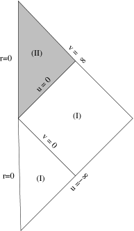
FIG. 6.: Conformal diagram for a typical naked singularity solution. The null surface $u=0$ separates the Minkowskian region (I) from the collapse region (II) where lies the time-like singularity at $r=0$.

REFERENCES

- [1] J. R. Oppenheimer and H. Snyder, Phys. Rev. D 56, 455 (1939).
- [2] D. Christodoulou, Commun. Math. Phys. 105, 337 (1986); 106, 587 (1986); 109, 591 and 613 (1987); Commun. Pure Appl. Math. XLIV 339 (1991); XLVI, 1131 (1993); Ann. Math. 140, 607 (1994).
- [3] M. W. Choptuik, Phys. Rev. Lett. 70, 9 (1993).
- [4] For a review of works in gravitational collapse, including scalar field collapse, see: T. P. Singh in Classical and Quantum Aspects of Gravitation and Cosmology ed. G. Date and B. R. Iyer (Institute of Mathematical Sciences, Madras, 1996), gr-qc/9606016 and A. Wang, Braz. J. Phys. 31, 188 (2001).
- [5] P. R. Brady, Class. Quantum Grav. 11, 1255 (1994).
- [6] Y. Oshiro, K. Nakamura and A. Tomimatsu, Prog. Theor. Phys. 91, 1265 (1994).
- [7] M. D. Roberts, Gen. Rel. Grav. 21, 907 (1989).
- [8] A. Wang and H. P. de Oliveira, Phys. Rev. D 56, 753 (1997).
- [9] C. W. Misner, K. S. Thorne and J. A. Wheeler, Gravitation, (Freeman, New York, 1973).
- [10] A. A. Coley, Class. Quantum Grav. 14, 87 (1997).
- [11] G. D. Birkhoff, Relativity and Modern Physics, (Harvard University Press, Cambridge, Mass., 1923).
- [12] R. Penrose, Revista del Nuovo Cimento 1, 252 (1969).
- [13] For a review see: R. M. Wald, Gravitational Collapse and Cosmic Censorship, gr-qc/9710068.
- [14] R. Penrose, in General Relativity, an Einstein Centenary Survey, eds. S. W. Hawking and W. Israel (Cambridge University Press, Cambridge, 1979).