RADIATION FROM BODIES WITH EXTREME ACCELERATION II: KINEMATICS

Abstract

When applied to a dipole source subjected to acceleration which is violent and long lasting (“extreme acceleration”), Maxwell’s equations predict radiative power which augments Larmor’s classical radiation formula by a nontrivial amount. The physical assumptions behind this result are made possible by the kinematics of a system of geometrical clocks whose tickings are controlled by cavities which are expanding inertially. For the purpose of measuring the radiation from such a source we take advantage of the physical validity of a spacetime coordinate framework (“inertially expanding frame”) based on such clocks. They are compatible and commensurable with the accelerated clocks of the accelerated source. By contrast, a common Lorentz frame with its mutually static clocks won’t do: it lacks that commensurability. Inertially expanding clocks give a physicist a window into the frame of a source with extreme acceleration. He thus can locate that source and measure radiation from it without being subjected to such acceleration himself. The conclusion is that inertially expanding reference frames reveal qualitatively distinct aspects of nature which would not be accessible if static inertial frames were the only admissible frames.

I INTRODUCTION

Minkowski spacetime with its Lorentz geometry is the geometrical framework for most physical measurements, in particular those involving radiation and scattering processes. Indeed, the asymptotic “in” and “out” regions of the scattering matrix, as well as the asymptotic “far-field” regions of a radiator reflect this fact.

If the scatterer or radiation source is accelerated linearly and uniformly, then the standard approach is to characterize its coaccelerating coordinate frame in terms of a one-parameter family of instantaneous Lorentz frames, any one of which provides the necessary “in” and “out” or “far-field” regions for the measurements of the scattered and emitted radiation.

However, suppose the acceleration is extreme, i.e.

• the acceleration, say $g$, lasts long enough for the scatterering/radiation source to acquire relativistic velocities and

• is large enough to do this within one cycle of its characteristic frequency $\omega$ so that

  $$\frac{g}{\omega}\sim\textrm{(speed of light)}~{}.$$

Under such a circumstance no physicist who insists on using a given asymptotic Lorentz frame as his observation platform can escape from a number of difficulties trying to execute his measurements.

First of all, there is the distortion problem. Relative to any Lorentz frame a signal emitted by, say, an accelerated dipole would be subjected to a time-dependent Doppler shift (“Doppler chirp”). The received signal starts out with an extreme blue shift and finishes with an extreme red shift. Such a distortion prevails not only in the time domain, but also in the spatial domain of that Lorentz frame. Once this distorted signal has been acquired by the observer in his Lorentz frame, he is confronted with the task of applying a time and/or space transformation to remove this distortion. He must reconstruct the signal in order to recover with 100% fidelity the original signal emitted by the source. Such a task is tantamount to changing from his familiar set of clocks and meter rods, which make up his Lorentz frame, to a new set of clocks and units of length relative to which the signal presents itself in undistorted form with 100% fidelity.

Second, there is the problem of the trajectory of the accelerated source. In order to have a “far field” region, the source must be much smaller than one wavelength. If the acceleration lasts long enough, the source will reach within one oscillation the asymptotically distant observer where the measuring equipment is located and thus vitiate its status as being located in the “far field” region: there no longer is large sphere that surrounds the source.

Finally, during such an acceleration process the source would be emitting plenty of information about itself (in the form of spectral power, angular distribution, etc.). However, to acquire this information the Maxwell field must be measured in the radiation zone. It lies outside a sphere centered around the source with radius one wave length. (Inside this sphere the radiation field is inextricably mixed up with the “induction” field.) Measuring the Maxwell field consists of relating its measured amplitude to the synchronized clocks and measuring rods. But this is precisely what cannot be done if the wavelength is larger than (acceleration)^-1 of the accelerated source. In that case the far field falls outside the semi-infinite domain Misner et al. (1973a) where the events are characterized uniquely by the clocks that are synchronized with the accelerated clock of the source. Put differently, the semi-finite size of the “local coordinate system of the accelerated source” Misner et al. (1973b) does not allow an observer to distance himself far enough from the source to identify the radiative field in the far zone.

Aside from removing the above ambiguities, the purpose of this note is to identify the spacetime framework which accommodates Maxwell’s field equations applied to a uniformly and linearly accelerated radiation source. One such application is the radiation observed in response to a dipole source. The observed radiation rate is given by the familiar Larmor formula but augmented due to the unique source-induced spacetime framework. This enhanced Larmor radiation formula is the result of a straightforward calculation based on this framework. There are no arbitrary hypotheses. The formula is given by Gerlach (2001):

$$\left(\begin{array}[]{c}\textrm{flow of radiant}\\ \textrm{energy into the}\\ \textrm{direction of acc'n}\end{array}\right)=\frac{2}{3}\left[\left(\frac{d^{2}D}{d\tau^{2}}\right)^{2}+\left(\frac{dD}{d\tau}\right)^{2}\right]$$ (1)

Here

$$D=\left(\begin{array}[]{c}\textrm{proper}\\ \textrm{dipole}\\ \textrm{moment}\end{array}\right)\times\left(\begin{array}[]{c}\textrm{proper acc'n}\\ \textrm{of the}\\ \textrm{dipole}\end{array}\right)$$

is the geometrical dipole moment. It is the time dependent magnitude of a dipole source pointing along the direction of acceleration, which is linear and uniform. Furthermore,

$$\tau=\left(\textrm{geometrical (dimensionless, ``Rindler'') time}\right)~{},$$

and the quantity

$$\left(\begin{array}[]{c}\textrm{flow of radiant}\\ \textrm{energy into the}\\ \textrm{direction of acc'n}\end{array}\right)=\left(\begin{array}[]{c}\textrm{linear density of}\\ \textrm{longitudinal component}\\ \textrm{of radiated momentum}\end{array}\right)~{}.$$

is defined by the conserved $\tau$-momentum in boost-invariant sector $F$,

$$\displaystyle\int_{-\infty}^{\infty}d\tau \overbrace{\int_{0}^{\infty}\int_{0}^{2\pi}T_{~{}\tau}^{\xi}\xi\,rdrd\theta}^{\textrm{evaluated at }\xi=const.\textrm{ in }F}=$$

$$\displaystyle\int_{-\infty}^{\infty}d\tau \left(\begin{array}[]{c}\textrm{linear density of}\\ \textrm{longitudinal component}\\ \textrm{of radiated momentum}\end{array}\right).$$

Formula (1) expresses a causal link between what happens at the accelerated source and the radiant energy observed on the other side of event horizon. The $\tau$-coordinate is the key. It is a symmetry trajectory on both sides of this horizon. This enables it to serve as the same standard for reckoning changes in the source in $I$ as for reckoning changes in the location in $F$.

What is the spacetime framework, i.e. the nature of the arrangement of measuring rods and clocks which makes this formula possible? Even if the spacetime framework for the accelerated dipole source is clear, comprehending Eq.(1) entails asking: (i) What is the spacetime framework for the observer who measures the radiation? (ii) What is the relationship between his framework and that of the source?

As depicted in Figure 1, the source traces out a world line which is hyperbolic relative to a globally free-float observer, one with a system of inertial clocks in a state of relative rest to one another. However, the observed energy given by Eq.(1) is to be measured by a different observer, one whose clocks, even though also inertial, have nonzero expansion relative to one another.

We shall find that the arrangement of clocks and rods of such an observer is confined to future sector $F$ of Figure 1. This sector is separated by the history of a one-way membrane (“event horizon”) from the spacetime domain, sector $I$, of the source. The purpose of this article is to establish a physical bridge between the two, and bolt them together into a single arena appropriate for the measurement of attributes of bodies subjected to extreme acceleration, Eq.(1) being one of them.

Figure 1: Acceleration-induced partitioning of spacetime into four boost-invariant sectors. They are centered around the reference event $(t_{0},z_{0})$ so that $U=(t-t_{0})-(z-z_{0})$ and $V=(t-t_{0})+(z-z_{0})$ are the retarded and advanced time coordinates for this particular quartet of boost (a.k.a. “Rindler”) sectors. The meaning of the boost coordinates $\xi$ and $\tau$ is inferred from the expressions for the invariant interval $-dt^{2}+dz^{2}=-\xi^{2}d\tau^{2}+d\xi^{2}$ in $I$ & $II$ and $-dt^{2}+dz^{2}=\xi^{2}d\tau^{2}-d\xi^{2}$ in $F$ & $P$. The emitted radiation given by Eq.(1) applies to a point-like source whose world line traces out the hyperbola in sector $I$.

The above questions do not deal with the inertia of bodies, nor with the dynamics of material particles, nor with the dynamics of the Maxwell field equations. Instead, they address kinematical aspects of the source and the observer by introducing geometrical clocks which are commensurable.

II GEOMETRICAL CLOCKS

The measurement of radiation and other electrodynamical processes depends on establishing a quantitative relationship ($x\rightarrow\vec{E}(x),\vec{B}(x)$) between the electromagnetic field and a coordinate reference system. Such a system consists of identically constructed clocks, which, for a freely floating reference system Taylor and Wheeler (1992), are (i) synchronized and (ii) separated by a standard unit (rigid meter rod) of length. However, measurements based on standard atomic clocks and on standard atomic units of length have a number of disadvantages.

First of all, they do not take advantage of the fact that the speed of light furnishes a unique and universal relation between the standard of time and the standard of length.

Second, for an accelerated reference system the (pseudo) gravitational frequency shift frustrates the synchronization of clocks indicating proper time.

Third, the pseudo gravitational redshift changes the wavelength of light and hence brings about discrepancies between the atomic standard of length based on a fixed number of wavelengths of Krypton 86 (more recently, of iodine stabilized He-Ne laser light) and the atomic standard based on a fixed number of platinum atoms (rigid platinum-iridium meter stick in Paris).

Last, but not least, there are regions which simply don’t lend themselves to being probed by rigid bodies, if for no other reason than that the assumed rigidity of material meter rods loses its meaning when the acceleration becomes high enough.

The methods of Doppler radar and pulse radar do not suffer from any of these disadvantages. Moreover, it is possible to formulate the entire kinematics of special relativity in terms of the methods of radar.

II.1 Radar Units

Fundamentally, physics, including the kinematics of moving bodies, is based on measurements. The class of measurements we shall focus on are those made by identically constructed “radar units”, each in its state of acceleration, which may be zero, in which case it is in a state of “free-float”. The meaning of “radar units” is that each one of them has

• a Doppler radar which emits a standard frequency wave train, controlled by an atomic clock of neglegible size (“atomic wrist watch”),

• a frequency analyzer capable of measuring and recording the Fourier spectrum of the reflected Doppler signal or of the pulse train emitted by another radar unit,

• a reflecting surface so as to make the radar unit visible to the radar of the other units,

• a coincidence pulse radar which consists of a transponder (receiver+transmitter), which upon receiving a pulse will emit without any delay a replica of this pulse, and

• a recording device which counts and is capable of storing the intensity of the received pulses.

The coincidence pulse capability implies that if there are two radar units, then a pulse striking one of them initiates a process of a pulse bouncing back and forth between the two radar units. This is depicted in Figures 2 and 3, where the two radar units are labelled A and B.

II.2 Fourier Compatibility

A fundamental property of every pair of radar units is their compatibility with respect to frequency measurements. More precisesly, one has the following definition:

Two radar units are said to be Fourier compatible if and only if a continuous wave train emitted by one radar unit produces a return signal which has a sharp Fourier spectrum at the second radar unit. If the return signal is not spectrally sharp (within prespecified bounds), then the two units are said to be Fourier incompatible.

A pair of Fourier compatible radar units, say A and B, is characterized by two frequency shift factors. The transmission process A $\rightarrow$ B is characterized by

$$k_{AB}\equiv$$

$$\frac{\textrm{(frequency of atomic clock at B)}}{\textrm{(frequency of atomic clock at A, but observed at B)}}~{},$$

while the reverse transmission process B $\rightarrow$ A is characterized by

$$k_{BA}\equiv$$

$$\frac{\textrm{(frequency of atomic clock at A)}}{\textrm{(frequency of atomic clock at B, but observed at A)}}~{}.$$

The numbers $k_{AB}$ and $k_{BA}$ are, of course, the familiar Doppler frequency shift factors if A and B are freely floating units, and the pseudo-gravitational frequency shift factors if A and B are uniformly and collinearly accelerated units. For the former one has $k_{AB}=k_{BA}$, while for the latter one has $k_{AB}=1/k_{BA}$.

These frequency shifts (“Fourier compatibility factors”) are strictly kinematical aspects of A and B. They involve neither the inertia nor the dynamics of material particles. Nevertheless, they do distinguish between free-float and acceleration. Indeed this distinction is encoded into the the relation between the frequency shifts associated with the reflection process A $\rightarrow$ B $\rightarrow$ A for monochromatic radiation. There one has

$$k_{A\rightarrow B\rightarrow A}\equiv k_{A\rightarrow B}k_{B\rightarrow A}=k_{AB}k_{BA}$$

$$=\left\{\begin{array}[]{cc}(k_{AB})^{2}&\begin{array}[]{c}\textrm{whenever A $\&$ B}\\ \textrm{are floating freely}\end{array}\\ {}\hfil&{}\hfil\\ 1&\begin{array}[]{c}\textrm{whenever A $\&$ B}\\ \textrm{are in states of}\\ \textrm{uniform collinear acc'n}\end{array}\end{array}\right.$$

For example, it is clear that all freely floating (“inertial”) units are Fourier compatible. So are the units which are linearly and uniformly accelerated and have the same future and past event horizons. However, an accelerated unit and one in a state of free float are not Fourier compatible. Neither are two units if one of them undergoes non-uniform acceleration. Such units measure a Doppler chirp instead of a constant Doppler shift when they receive the wave train reflected by the other.

II.3 Geometrical Clocks

Time and space acquire their meaning from measurements, i.e. identifications of a relationship by means of a unit that serves as a standard of measurement. The measurement process we shall focus on is based on the emission, reflection, and reception of radar pulses generated by a standard geometrical clock.

Such a clock consists of a pair of Fourier compatible radar units, say, A and B. Their reflective surfaces form the two ends of a one-dimensional cavity with its evenly spaced spectrum of allowed standing wave modes in between. The operation of the geometrical clock hinges on having an electromagnetic pulse travel back and forth between the reflective ends of the cavity. The back and forth travel rate is determined by the separation between the cavity ends. This rate need not, of course, be constant in relation to the atomic clocks carried at either end. A geometrical clock with mutually receding ends would exemplify such a circumstance.

The definition of a geometrical clock is therefore this: it is a one-dimensional cavity

• whose bounding ends are Fourier compatible and

• which accommodates an electromagnetic pulse bouncing back and forth between the left and right end of the cavity.

This bouncing action forms the tick-tock events of the clock. If the cavity is expanding inertially, these events are located at

$$\begin{array}[]{clc}(t,z)=be^{n\Delta\tau}&(1,0)&\left(\begin{array}[]{c}n=\textrm{even}\\ \textrm{``tick''}\end{array}\right)\\ (t,z)=be^{(n+1)\Delta\tau}&(\cosh\Delta\tau,\sinh\Delta\tau)&\left(\begin{array}[]{c}n+1=\textrm{odd}\\ \textrm{``tock''}\end{array}\right)\end{array}$$ (6)

along the two straight world lines of radar units A and B in spacetime sector $F$. Here

$$e^{\Delta\tau}=k_{AB}$$

is the Doppler frequency shift factor and $\Delta\tau$ is the fixed comoving separation between A and B. The constant $b$ is the Minkowski time when the geometrical clock strikes zero.

For a clock with ends subjected to accelerations $1/b$ and $1/be^{\Delta\tau}$, the ticking events are located at

$$\begin{array}[]{clc}(t,z)=b&(\sinh n\Delta\tau,\cosh n\Delta\tau)&\left(\begin{array}[]{c}n=\textrm{even}\\ \textrm{``tick''}\end{array}\right)\\ (t,z)=be^{\Delta\tau}&(\sinh(n+1)\Delta\tau,\cosh(n+1)\Delta\tau)&\left(\begin{array}[]{c}n+1=\textrm{odd}\\ \textrm{``tock''}\end{array}\right)\end{array}$$ (7)

along the two hyperbolic world lines of A and B in boost-invariant sector $I$. Here

$$e^{\Delta\tau}=k_{AB}$$

is the pseudo-gravitational frequency shift factor between them, and $\Delta\tau$ is the boost time between a “tick” and a “tock”.

The spacetime history of such clocks and their bouncing pulses are exhibited in Figures 2 and 3.

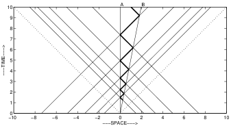
Figure 2: Spacetime history of an inertially expanding clock and the null trajectories of trains of emitted and received pulses (light lines) whose emission and reception is controlled by the internal pulse (heavy line) bouncing back and forth between A and B.

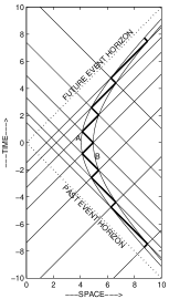
Figure 3: Spacetime history of an accelerated clock and the null trajectories of trains of emitted and received pulses (light lines) whose emission and reception is controlled by the internal pulse (heavy line) bouncing back and forth between A and B.

To serve its purpose, a geometrical clock AB emits and receives pulses of radiation. When the internal pulse strikes radar unit A its transmitter and its receiver are turned on only for the duration of the pulse. This causes A to emit a pulse and to register the reception of a pulse from the outside, if there is one coming. When the internal pulse has bounced back to B, an analogous emission and reception process takes place at radar unit B. It follows that that the tick-tock action of the internally bouncing clock pulse determines a set of external pulses moving to the right and to the left. The history of these pulses together with the clock that controls them is depicted by Figures 2 and 3 for an inertially expanding and accelerating clock respectively.

III PRINCIPLES OF MEASUREMENT

Geometrical clocks play a fundamental role in the development of the measurement of space and time. However, in order not to appear arbitrary, following Rand and Peikoff, we shall remind ourselves telegraphically of the nature of measurement from a perspective which requires no specialized knowledge and no specialized training.

A process of measurement involves two concretes: the thing being measured and the thing that is the standard of measurement. The relationship between the two is reciprocal: either one may serve as a standard. Measurements pertain to the attributes of these concretes. The choice of one of them as a standard is based on having its attribute serve as a unit of measurement. The process of measurement consists of establishing a relationship to this unit which serves as a standard of measurement.

Within certain limits the choice of a standard is optional. However, the primary standard must be in a form (e.g. platinum meter rod in Paris, or Cesium clock at N.I.S.T. in Boulder, Colorado, etc.) easily accessible to a physicist and it must represent the specific attribute which serves as a unit of measurement (e.g. 1 meter of length, or 1 second = 9,192,631,770 Cesium cycles of time, etc.). Moreover, once a standard has been chosen, it becomes immutable for all subsequent measurements. Any chosen standard satisfies this principle. A standard gets copied in the form of secondary standards. Their purpose is to establish – usually by a process of counting – a quantitative relationship between the standard and any other instance of the attribute of the thing to be measured.

Whenever certain concretes have attributes which can be related to the same standard of measurement, one says that these concretes are commensurable. The importance of commensurability lies in the fact that it is an equivalence relation: If concrete $\mathcal{A}$ is commensurable with concrete $\mathcal{B}$, then $\mathcal{B}$ is commensurable with $\mathcal{A}$; if $\mathcal{A}$ is commensurable with $\mathcal{B}$, and $\mathcal{B}$ is commensurable with $\mathcal{C}$, then $\mathcal{A}$ is commensurable with $\mathcal{C}$. Using this fact, and omitting explicit reference to the specific measurement of their attributes, but retaining their existence, a physicist integrates these concretes into an equivalence class.

Thus, based on commensurability with a standard rod, one forms an equivalence class, the concept length. Or, based on commensurability with an entity undergoing a periodic process, one forms another equivalence class, the concept time.

A century ago physicists thought that the concept of length and of time required two independent standards, one for each. But in 1905 it was realized that these two standards are not independent. In fact, they are related by a universal conversion factor, the speed of light in vacuum. Thus starting in 1983 both length and time have been defined by referring to a single standard, a unit of time as determined by the tickings of a Cesium atomic clock.

By having such a clock control the pulse repetition rate of a mode-locked femtosecond-laser, one generates a phase-coherent train of pulses Udem et al. (2002). Introduce this train into the one-dimensional resonance cavity of a geometrical clock with ends at relative rest as shown in Figure 4. A resonance condition is obtained when (twice) the length of that cavity is adjusted to equal the spacing in that train of pulses. This resonance condition accomplishes two things:

1. It establishes the relationship between a Cesium-controlled standard of time, i.e. the duration between successive femtosecond pulses, and the corresponding standard of length, i.e. the size of the resonance cavity.

2. It makes the geometrical clock into a single representative of a standard of time and of the space measurements. The periodic tickings of the pulse bouncing back and forth inside provides copies of that standard of time, while the adjusted cavity size furnishes that standard of length.

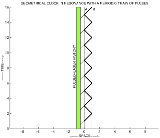
Figure 4: Free-float geometrical clock driven at resonance by a periodic train of pulses. The partial transmissivity of partial reflector A admits part of their amplitude into the interior of geometric clock AB. When their period matches the reflection time inside the clock, resonance prevails, and they form a single pulse which bounces back and forth (heavy zig-zag line) inside AB. This bouncing is the ticking of the geometrical clock. The ticking interval is the standard of time, while the spatial extent of AB is the associated standard of length. Note that the picture omits, among others, the laser pulses reflected from A and the partially transmitted pulses emerging from B.

IV COMMENSURABILITY

Recall that a geometrical clock is defined as a pair of radar units whose emission of monochromatic wave trains yields two well defined mutual frequency shift factors ($k_{AB}$ at B and $k_{BA}$ at A) and whose reflective surfaces support an electromagnetic pulse bouncing back and forth between them.

Geometrical clocks differ from one another by virtue of their differing frequency shift factors and hence their differing ticking rates. Moreover, these rates are in general not even uniform. Nevertheless a comparison of these clocks is possible. The general idea is to consider the ratio of their ticking rates. These ratios open the door to identifying a commensurable property even among certain geometrical clocks which run nonuniformly relative to their resident atomic clocks. The implementation of this endeavor is best done in two steps: first for adjacent clocks, then for distant ones.

IV.1 Adjacent Clocks

To compare the operation of two adjacent geometrical clocks, AB and BC one notes that they have radar unit B in common. Assume that all three radar units A, B, and C move collinearly along the $z$ axis. The common radar unit B has electromagnetic pulses bouncing off it. There are those from A and those from C. Consider $a$ consecutive pulses from A and $c$ consecutive pulses from C:

$$\begin{array}[]{c}{}\hfil\\ \textrm{pulses at B coming from A:}{}{}{}{}\end{array} \begin{array}[]{c}{}\hfil\\ \bullet\end{array}\cdots~{}\begin{array}[]{c}p_{i}\\ \bullet\end{array}\overbrace{\begin{array}[]{c}p_{i+1}\\ \bullet\end{array}\begin{array}[]{c}p_{i+2}\\ \bullet\end{array}\begin{array}[]{c}p_{i+3}\\ \bullet\end{array}~{}\cdots~{}\begin{array}[]{c}p_{i+a}\\ \bullet\end{array}}^{a}~{}\begin{array}[]{c}p_{i+a+1}\\ \bullet\end{array}~{}\cdots~{}\begin{array}[]{c}{}\hfil\\ \bullet\end{array}\cdots$$

$$~{}~{}~{}~{}~{}~{}\rule[2.27621pt]{99.58464pt}{0.45525pt}~{}\textrm{(time)}~{}\rule[2.27621pt]{99.58464pt}{0.45525pt}\!\!\!\!\!\!\rightarrow~{}$$

$$\begin{array}[]{c}{}\hfil\\ \textrm{pulses at B coming from C:}{}{}{}{}\end{array} \begin{array}[]{c}{}\hfil\\ \bullet\end{array}\cdots\,\begin{array}[]{c}~{}q_{j}\\ \bullet\end{array}~{}\underbrace{\begin{array}[]{c}~{}q_{j+1}\\ \bullet\end{array}~{}~{}~{}\begin{array}[]{c}q_{j+2}\\ \bullet\end{array}\begin{array}[]{c}{}\hfil\\ {}\hfil\end{array}\cdots~{}\begin{array}[]{c}q_{j+c}\\ \bullet\end{array}}_{c}\begin{array}[]{c}q_{j+c+1}\\ \bullet\end{array}~{}\cdots~{}\begin{array}[]{c}{}\hfil\\ \bullet\end{array}\cdots~{}.$$

These sequences are depicted in Figures 5 and also in 6. We say that these two sequences are matched relative to B, and we write

$$\{p_{i},p_{i+1},\cdots,p_{i+a}\}_{B}\sim\{q_{j},q_{j+1},\cdots,q_{j+c}\}_{B}~{},$$

if and only if they have – within a prespecified accuracy – coincident starting ($p_{i}$ and $q_{j}$) and coincident termination ($p_{i+a}$ and $q_{j+c}$) pulses. The subscript B on these sequences serves as a reminder that the pulses are being counted at radar unit B.

The electromagnetic pulses impinging on B get partially reflected and partially transmitted. Thus for every pulse sequence $\{p_{i},p_{i+1},\cdots,p_{i+a}\}_{B}$ measured at B there are corresponding sequences $\{p_{i},p_{i+1},\cdots,p_{i+a}\}_{A}$ and $\{p_{i},p_{i+1},\cdots,p_{i+a}\}_{C}$ measured at A and C respectively. Thus one has the following proposition (“Invariance of matched sequences”):

The property of being matched is invariant as each sequence of pulses travels from one radar unit to another, i.e. if

$$\{p_{i},p_{i+1},\cdots,p_{i+a}\}_{B}\sim\{q_{j},q_{j+1},\cdots,q_{j+c}\}_{B}~{},$$

then

$$\{p_{i},p_{i+1},\cdots,p_{i+a}\}_{A}\sim\{q_{j},q_{j+1},\cdots,q_{j+c}\}_{A}$$

and

$$\{p_{i},p_{i+1},\cdots,p_{i+a}\}_{C}\sim\{q_{j},q_{j+1},\cdots,q_{j+c}\}_{C}~{}.$$

The validity of this proposition is an expression of the principle of the constancy of the speed of light, that is, of the fact that light pulses cannot overtake each other. If two pulses, say $p_{i}$ and $q_{j}$, are coincident on the world line of radar unit B, then they are still coincident after they have travelled to the world line of any other radar unit, regardless of its motion.

As measured by atomic clock B, the ticking rates of geometrical clocks AB and BC need not be uniform, and in general they are not. This is evident from Figure 5. This deficiency is remedied by calibrating the rate of pulses coming from C in terms of AB. Thus for every $c$-sequences of pulses departing from C and arriving and counted at B, there is a matched $a$-sequence generated by clock AB also at B. The ratio

$$\frac{c}{a}=\frac{\textrm{(\# of ticks of clock BC)}}{\textrm{(\# of ticks of clock AB)}}$$ (10)

is the normalized ticking rate of clock BC. The normalization is relative to clock AB. Conversely, the inverse of Eq.(10),

$$\frac{a}{c}=\frac{\textrm{(\# of ticks of clock AB)}}{\textrm{(\# of ticks of clock BC)}}$$ (11)

is the ticking rate of AB normalized relative to BC. Because of the invariance of matched sequences, it does not matter whether the ratios, Eqs.(10)-(11), were measured at radar unit A, B, or C.

We say that the adjacent clocks AB and BC are normalizable if both ratio (10) and ratio (11) are non-zero for every matched pair of $a$ and $c$-sequences along the world lines of the two adjacent clocks. A basic and obvious aspect of normalizability for adjacent clocks is its reciprocal property: If AB is normalizable relative to BC, then BC is normalizable relative to AB. Thus all collinear clocks AB, BC, BD, BE, $\cdots$, which share radar unit B, are mutually normalizable.

Of particular utility are clocks which are commensurable. Their distinguishing property is obtained by subdividing the set of normalizable geometrical clocks further and selecting those whose normalized ticking rates, Eq.(10) or (11), are constant for all matched starting and termination pulses. Such clocks allow one to view the boost-invariant accelerated and the boost-invariant expanding inertial frames from a single perspective, which is developed in Section VII.

Before giving the precise general definition of commensurability (Section IV.2, we interrupt the developement by illustrating the above constellation of definitions, applying them to various combinations of inertial and accelerated clocks.

Nota bene: For the purpose of verbal shorthand we shall allow ourselves to refer to “geometrical clocks” simply as “clocks”. However, for atomic clocks we shall use no such shorthand. Thus clocks without the adjective “atomic” are understood to be geometrical clocks, while atomic clocks are always referred to by means of the modifier “atomic”.

IV.1.1 Commensurable Inertial Clocks

Consider a pair of clocks AB and BC, where all three radar units A, B, and C are freely floating, and radar unit B is common to AB and BC, as in Fig. 5.

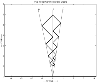
Figure 5: Two adjacent geometrical clocks consisting of inertially expanding cavities AB and BC, each containing a pulse bouncing back and forth. Depicted in this diagram are sequences of 2 pulses coming from A and impinging on B which are matched by corresponding sequences of 3 pulses coming from C. The ratio $c/a=3/2$ is the ticking rate of BC normalized to that of AB. The fact that this ratio stays constant throughout the history of the two clocks makes them commensurable.

What is the ratio $c/a$ of two matched pulse sequences impinging on radar unit B and coming from radar units A and C? This ratio is determined by the following mini-calculation:

Let A emit two pulses separated by

$$\Delta\xi$$

as measured by atomic clock A. Due to the relative motion of A and B these two pulses, once received at B, have time separation

$$k_{AB}\Delta\xi$$

as measured by atomic clock B. Here $k_{AB}$ is a positive (“Doppler”) factor whose magnitude expresses the motion of A relative to B. There are now two time intervals: the one between the emitted pulses and the one between the received pulses. These intervals are proportional to the wavelengths of emitted and received monochromatic radiation. Their ratio,

$$\frac{k_{AB}\Delta\xi}{\Delta\xi}=k_{AB}$$

is the Doppler shift factor. The two radar units are understood to be at rest relative to each other whenever $k_{AB}=1$. They are receding (resp. approaching) each other whenever $k_{AB}>1$ (resp. $k_{AB}<1$), which expresses a Doppler red (resp. blue) shift. It is clear that this Doppler shift of clock AB controls the rate at which the back-and-forth bouncing pulse produces ticks at radar unit B. In fact, the pulse arrival times of $a$ consecutive pulses coming from A are

$$\xi,\,k_{AB}^{2}\xi,\cdots,\,k_{AB}^{2a}\xi.$$

Similarly, the arrival times of $c$ consecutive pulses coming from radar unit C, which is part of clock BC, are

$$\xi,\,k_{BC}^{2}\xi,\cdots,\,k_{BC}^{2c}\xi.$$

These two pulse sequences have coincident initial pulse arrival times $\xi$. If these two sequences are “matched”, then their final pulse arrival times, $k_{AB}^{2m}\xi=k_{BC}^{2n}\xi$, also coincide. Under this circumstance the length of these two pulse sequences as measured by atomic clock B are the same. Consequently,

$$k_{AB}^{2a}\xi-\xi=k_{BC}^{2c}\xi-\xi,$$

or

$$\frac{c}{a}=\frac{(1/\log k_{BC})}{(1/\log k_{AB})}.$$ (12)

This is the ticking rate of clock CB normalized relative to clock AB. This ticking rate is a constant independent of the starting time $\xi$ of the two matched pulse sequences. Consequently, clock AB is commensurable with BC.

IV.1.2 Commensurable Accelerated Clocks

Again consider a pair of clocks AB and BC.

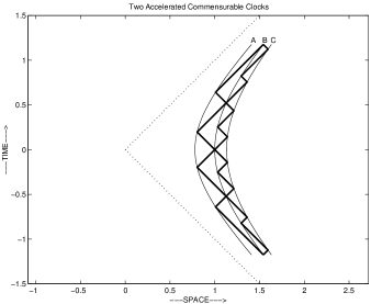
Figure 6: Two adjacent geometrical clocks consisting of collinearly accelerated cavities AB and BC, each containing a pulse bouncing back and forth. Depicted in this diagram is a sequence of 4 pulses coming from A and impinging on B which are matched by a sequence of 8 pulses coming from C. The ratio $c/a=8/4$ is the ticking rate of BC normalized to that of AB. The fact that this ratio stays constant throughout the history of the two clocks makes them also commensurable, just like those in Figure 5

But this time have all three of their radar units accelerate collinearly to the right with respective constant accelerations $1/\xi_{A}$, $1/\xi_{B}$, and $1/\xi_{C}$ respectively, and with common future and past event horizons, as in Figure 6. To make the discussion concrete, assume that $0<\xi_{A}<\xi_{B}<\xi_{C}$.

Consider the ticking produced by a pulse bouncing back and forth in clock AB. The proper time between two successive ticks at A is

$$\xi_{A}\times\left(\begin{array}[]{c}\textrm{boost coordinate}\\ \textrm{time between ticks}\end{array}\right)=\xi_{A}\times 2\log(\xi_{B}/\xi_{A})~{},$$

while at B it is

$$\xi_{B}\times\left(\begin{array}[]{c}\textrm{boost coordinate}\\ \textrm{time between ticks}\end{array}\right)=\xi_{B}\times 2\log(\xi_{B}/\xi_{A})~{},$$

Their ratio

$$\frac{2\,\xi_{B}\log(\xi_{B}/\xi_{A})}{2\,\xi_{A}\log(\xi_{B}/\xi_{A})}=\frac{\xi_{B}}{\xi_{A}}\equiv k_{AB}$$ (15)

is the pseudo-gravitational frequency shift factor. Similarly, for clock BC one has

$$\frac{\xi_{C}}{\xi_{B}}\equiv k_{BC}~{}.$$ (16)

These two frequency shift factors control the rate at which pulses arrive at B from A and C respectively. In fact, the two corresponding matched pulse sequences are

$$0,2\,\xi_{B}\log(\xi_{B}/\xi_{A}),\cdots,2\,a\xi_{B}\log(\xi_{B}/\xi_{A})$$

and

$$0,2\,\xi_{B}\log(\xi_{C}/\xi_{B}),\cdots,2\,c\xi_{B}\log(\xi_{C}/\xi_{B})~{},$$

where the last pulse arrival time is the same, i.e.

$$2\,a\xi_{B}\log(\xi_{B}/\xi_{A})=2\,c\xi_{B}\log(\xi_{C}/\xi_{B})~{},$$

or with the help of Eqs.(15) and (16)

$$\frac{c}{a}=\frac{(1/\log k_{BC})}{(1/\log k_{AB})}~{}.$$ (17)

This is the ticking rate of clock BC normalized relative to clock AB. This ticking rate is a constant independent of the starting time of the two matched pulse sequences. Consequently, accelerated clocks AB and BC are also commensurable.

IV.2 Distant Clocks

To compare the operation of two distant clocks, AB and CD, note that they have four different radar units. Assume them to be moving collinearly along the $z$-axis such that A and D are the outer pair, and B and C the inner pair, as in Figures 7 and 8

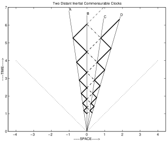
Figure 7: Two distant inertially expanding geometrical clocks. Clock CD can be calibrated in terms of AB because CD and AB are commensurable: Taking into account the ticking rate of the intermediate clock BC, one sees that the ratio of their rates is a constant, namely 1:1. Because this ratio happens to be unity, these two commensurable clocks are said to have the additional property of being identically constructed.

One says that two distant (nonadjacent) clocks AB and CD are commensurable, or more briefly

$$AB\approx CD~{},$$

if and only if

• Radar units A and B are visible for all times to radar units C and D and

• AB is commensurable with BC, and BC is commensurable with CD.

Being “visible” means that, by using its pulse radar, C can always see B on its radar screen, i.e. BC forms a geometrical clock. Thus two clocks AB and CD are commensurable if the clock formed by radar units B and C is commensurable with both of its neighbors, AB and CD.

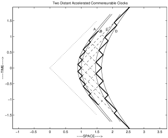
Figure 8: Two distant accelerated geometrical clocks. Clock CD can be calibrated in terms of AB because CD and AB are commensurable: Taking into account the ticking rate of the intermediate clock BC, one sees that the ratio of their rates is $\frac{1}{3}\times\frac{3}{1}=\frac{1}{1}$ in this figure. Because this ratio happens to be unity, these two commensurable clocks are said to have the additional property of being identically constructed.

According to this definition, one uses the constancy of the rate of clock CD normalized to that of clock BC,

$$\frac{(1/\log k_{CD})}{(1/\log k_{BC})}=const~{},$$

and the constancy of the rate of clock BC normalized to that of clock AB,

$$\frac{(1/\log k_{BC})}{(1/\log k_{AB})}=const~{},$$

to establish that the rate of clock CD normalized to that of clock AB,

$$\frac{(1/\log k_{CD})}{(1/\log k_{AB})}=const~{},$$ (18)

is also a constant, and therefore that CD is commensurable with AB. One sees from Eqs.(12) and (17) that this criterion for commensurability holds for both inertial and accelerated clocks, as is depicted in Figures 7 and 8.

Commensurability of distant clocks subsumes that of adjacent clocks as a special case. This follows from simply letting the space between clocks AB and CD in Figures 7 and 8 shrink to zero so that the final result is two adjacent clocks as in Figures 5 and 6. The commensurability is readily preserved throughout this limiting process.

Commensurability is a relation which satisfies the following three properties:

1. AB $\approx$ AB

2. AB $\approx$ CD implies CD $\approx$ AB

3. AB $\approx$ CD together with CD $\approx$ EF implies AB $\approx$ EF

A physicist can choose one of these commensurable clocks as his primary standard. It is a dual function device : It represents a temporal standard and a spatial standard at the same time. The spatial extent of the clock is determined uniquely by its ticking rate, a light pulse bouncing back and forth between the clock’s two ends.

V MEASURING EVENTS VIA RADAR

Assume the physicist has chosen a standard clock whose cavity ends have relative frequency shift factor

$$k_{AB}\equiv e^{\Delta\tau}~{}.$$

This Fourier compatibility factor controls the clock rate, which in turn controls the times that outgoing pulses leave the clock and the times that the receiver is turned on to allow the reception and recording of incoming pulses.

Events have a commensurable property, a property which is reducible (by a process of counting) to a standard of length and of time. The common method of measuring events, and historically the first, relies on counting replicas of a standard of length and synchronized replicas of a standard of time in order to identify an event in terms of coordinates. The standard of length and of time were considered distinct and independent of each other. But Einstein, by a process of hard work, noticed that (i) it takes an act of using ones visual faculties, and hence a familiarity with the properties of light, and that (ii) one must have a clear understanding of what is meant by “looking at clocks which are synchronized”, before one can claim to have measured an event.

With that observation it became clear that the standard of length and the standard of time cannot be chosen independently, but are related by the speed of light.

Suppose radar had been invented before 1905. Then using the method of radar to measure events would have forced a physicist to confront and solve the problem of using synchronized clocks before 1905. He would have immediately found from his observations that the standard of length is related to the standard of time. Further more, by following Bondi Trautman et al. (1965), the physicist would have immediately formulated the kinematics of special relativity, saving himself the hard work that Einstein had to do.

Both the method of radar and the common method for measuring an event have been formulated for radar sets, clocks, and measuring rods which are unaccelerated and static relative to one another. Can one extend these two formulations and will they remain equivalent if on drops these restrictions? The following sections give an affirmative answer.

V.1 The Radar Method

Let $n_{1}$ be the integer that labels a pulse emitted by radar unit B. If that pulse gets reflected, or partially reflected, by a scattering event, then let $n_{2}$ be the integer which the clock assigns to the reflected pulse as it enters the radar receiver. These two integers,

$$(n_{1},n_{2})~{},$$ (19)

generated by this radar ranging process are the radar coordinates of the scattering event. They assign a unique spacetime location to the scattering event, namely $(t,z)$ as determined by

$$\begin{array}[]{cc}T_{1}-Z_{1}=t-z&\textrm{(pulse moving to the right)}\\ T_{2}+Z_{2}=t+z&\textrm{(pulse moving to the left)}\end{array}$$ (20)

Here $(T_{1},Z_{1})$ and $(T_{2},Z_{2})$ are those two events at radar unit B which mark the emission and the reception of a pulse at B.

V.1.1 Inertially Expanding Clock

If B is controlled by the ticking of an inertially expanding clock, then these events are

$$(T,Z)=be^{n\Delta\tau}(1,0),~{}~{}~{}~{}~{}~{}~{}n=n_{1},n_{2}~{}.$$

These two events are marked by a square and a diamond in Figure 9. The constant $b$ is the proper time corresponding to $n=0$.

It follows from Eqs.(20) that the scattering event measured by B is

$$(t,z)=$$

$$be^{\Delta\tau(n_{1}+n_{2})/2}\left(\cosh\frac{n_{2}-n_{1}}{2}\Delta\tau~{},~{}\sinh\frac{n_{2}-n_{1}}{2}\Delta\tau\right)$$

These three events, $(T_{1},Z_{1})$, $(t,z)$ and $(T_{2},Z_{2})$, are marked in Figure 9 by a square, a circle, and a diamond.

V.1.2 Accelerated Clock

Similarly, if B is controlled by an accelerated clock, then the corresponding three events are

$$(T,Z)=b(\sinh{n\Delta\tau},\cosh{n\Delta\tau}),~{}~{}~{}~{}~{}~{}~{}n=n_{1},n_{2}~{}.$$

and

$$(t,z)=$$

$$be^{\Delta\tau(n_{1}-n_{2})/2}\left(\sinh\frac{n_{2}+n_{1}}{2}\Delta\tau~{},~{}\cosh\frac{n_{2}+n_{1}}{2}\Delta\tau\right).$$

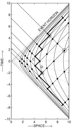
Figure 10: Lattice of spacetime graduation events (heavy dots) as determined and calibrated by a single geometrical clock CD which is accelerating. The spacetime history of the e.m. pulse bouncing inside this clock is the heavy zig zag line between the two hyperbolas C and D. The clock is bounded by these two hyperbolas, the histories of the two accelerating reflectors which keep the e.m. pulse trapped inside the clock. The other hyperbolas indicate the accelerated reflector histories of identically constructed clocks, if they were to form an array of adjacent geometrical clocks. The straight lines (lightly dotted) are the times simultaneous with the tickings of the standard clock CD. The 45⁰ lines emanating to the left from C and to the right from D are the histories of the two trains of pulses escaping from C and D, with those escaping from C ultimately crossing the event horizon of clock CD. The fact that CD is a standard clock implies that all graduation events of the calibrated lattice lie on these histories. Based on the method of pulsed radar, each graduation event (e.g. the encircled dot) is labelled by two unique integers, namely two numbered ticks (the dots in the square and in the diamond) of the clock. They are CD’s “radar coordinates” of that graduation event.

They are marked in an analogous way in Figure 10.

Equation (V.1.1) or (V.1.2) relates in mathematical form a scattering event to the ticking of a single geometrical clock chosen as a standard. This relationship has been established by the method of radar in terms of the integers $n_{1}$ and $n_{2}$.

V.2 The Common (Non-Radar) Method

There is, of course, the more common and familiar method. It does not use radar. Instead, it uses two distinct standards, namely, identically constructed clocks and standard rods Taylor and Wheeler (1992). The measuring procedure itself, we recall, consists of (i) locating the event by counting standard rods, and (ii) determining its time by counting at that location the ticks of the clock, which is synchronized to the standard clock.

One is now confronted with a question of consistency: Is this common non-radar method compatible with the radar method, even if the spacetime framework is based on inertially expanding or accelerated clocks?

Consider the common method of measuring an event. It consists of starting with a geometrical clock having a spacetime history as depicted in Figure 2 or 3. Such a clock is a standard of time and of length. Thus a physicist forms a spatial array of adjacent clocks AB, BC,$\cdots$, EF,$\cdots$ which are identically constructed and synchronized. The definition is as follows:

• Clocks AB, XY, $\cdots$ are said to be identically constructed if their frequency shift factors are all the same:

  $$k_{AB}=k_{XY}=\cdots\equiv e^{\Delta\tau}~{}.$$ (23)

This definition is illustrated in Figures 7 and 8.

The ticking of adjacent clocks is synchronized by synchronizing the pulses impinging on their shared radar unit. This procedure guarantees synchronization of all clocks. It is exemplified in Figure 7. There the three clocks AB, BC, and CD have the phases of their internal pulses adjusted to tick in synchrony.

Suppose standard clock AB has its $n$th (resp. $(n+1)$st) ticking event at its left (resp. right) radar unit A (resp. B). These events are exhibited by Eq.(6) or (7). Then, by induction, the left radar unit of the $M$th identically constructed clock has its $N$th ticking event at

$$(t,z) = be^{N\Delta\tau}\left(\cosh M\Delta\tau~{},~{}\sinh M\Delta\tau\right)~{}~{}~{}~{}(\textrm{for the }M\textrm{th inertially expanding clock})$$ (24)

$$(t,z) = be^{M\Delta\tau}\left(\sinh N\Delta\tau~{},~{}\cosh N\Delta\tau\right)~{}~{}~{}~{}(\textrm{for the }M\textrm{th accelerated clock})$$ (25)

Having formed a linear array of such clock, the physicist uses the lattice of events generated by their tick-tock actions as a standard to measure an arbitrary event. The common method of measuring an event consists of counting (i) how many clocks separate it from the standard clock ($M=0$), and (ii) how many clock ticks elapse before this event happens. The result of these two counts is the pair of integers

$$\begin{array}[]{cc}M=m&\left(\begin{array}[]{c}\textrm{result of}\\ \textrm{spatial measurement}\end{array}\right)\\ {}\hfil&{}\hfil\\ N=n&\left(\begin{array}[]{c}\textrm{result of}\\ \textrm{temporal measurement}\end{array}\right).\end{array}$$ (26)

They comprise the measurement of the given event in units of time and spatial extent as furnished by the standard geometrical clock.

V.3 Its Equivalence With The Radar Method

Now compare Eq.(24) with Eqs.(26) and (V.1.1) or Eq.(25) with Eqs.(26) and (V.1.2). Observe that for both cases

$$m = \frac{n_{2}-n_{1}}{2}$$ (27)

$$n = \frac{n_{2}+n_{1}}{2}~{}.$$ (28)

One sees that the radar method is equivalent to the common method provided one identifies the radar pulse data $(n_{2}-n_{1})/2$ with the $m$th distant clock, and $(n_{2}+n_{1})/2$ with its $n$th ticking event. This equivalence is new. It extends the fundamental and familiar result based on a lattice array of free-float clocks to (i) the case of an array of inertially expanding clocks and to (ii) the case of a array of accelerated clocks. Put differently, it gives physical validity to the concepts “inertially expanding frame” and “accelerated frame”.

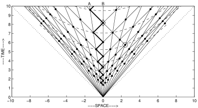
Figure 9: Lattice of spacetime graduation events (heavy dots) determined and calibrated by a single geometrical clock AB which is expanding inertially. The spacetime history of the e.m. pulse bouncing inside this clock is the heavy zig zag line left of the middle. The clock is bounded by two straight lines A and B, the histories of the receding reflectors which keep the e.m. pulse trapped inside the clock. The other straight lines indicate the receding reflector histories of identically constructed clocks, if they were to form an array of adjacent geometrical clocks. The hyperbolas (dashed lines) are the times simultaneous with the tickings of the standard clock AB. The 45⁰ lines emanating to the left from A and to the right from B are the histories of the two trains of pulses escaping from A and B. The fact that AB is a standard clock implies that all graduation events of the calibrated lattice lie on these histories. Based on the method of pulsed radar, each graduation event (e.g. the encircled dot) is labelled by two unique integers, namely two numbered ticks (the dots in the square and in the diamond) of the clock.They are AB’s “radar coordinates” of that graduation event.

VI IDENTICALLY CONSTRUCTED CLOCKS AS SYMPATHETICALLY RESONATING CAVITIES

The existence of identically constructed clocks – or entities which have the properties of such clocks – is essential for establishing a coordinate frame. This is true not only for coordinate frames which are freely floating, but also for those which are based on clocks which are inertially expanding or accelerated.

One’s success in realizing such clocks in the laboratory or identifying them nature is increased considerably by the fact that their existence is a manifestation of sympathetically resonating cavities.

This resonance behavior occurs when radiation is trapped in two weakly interacting cavities with identical normal mode spectra. This behavior plays the decisive role in the operation and synchronization of these clocks. There are two complementary, but equivalent, ways of understanding sympathetic resonance: in terms of travelling pulses and in terms of normal modes.

VI.0.1 Travelling Pulses

Consider two identically constructed clocks AB and CD, which are characterized by the same frequency shift factors $k_{AB}$ and $k_{BA}$:

$$\begin{array}[]{c}k_{AB}=k_{CD}\\ k_{BA}=k_{DC}\end{array}$$ (29)

Each of Figures 7 and 8 is an example of the spacetime history of two such clocks.

Let e.m. pulses from the first ticking clock enter, by partial transmission, the empty cavity of the second clock, which is initially not ticking (no e.m. pulse inside). Then these entering pulses will start a ticking process in this clock. Because of Eq.(29), this process is in perfect synchrony with the impinging pulses. They come precisely at the right moment and have the right phase so as to augment the interior pulse amplitude from one tick to the next . As a result, CD starts ticking in sympathy with AB.

If there is no event horizon between the two clocks, then the process can be reversed, and AB ticks in sympathy with CD. When both processes happen simultaneously, we say that the sympathetic resonance of AB and CD is mutual. In that case the pulses carry information both ways. This allows the synchronization of the two identically constructed clocks.

VI.0.2 Normal Modes

The complementary, but equivalent (via Fourier synthesis), perspective on this resonance is to note that the two clocks have identical normal mode spectra. More explicitly, the cavities have their ends moving in such a way that the normal modes, which are governed by the wave equation

$$-\frac{1}{\xi^{2}}\frac{\partial^{2}\psi}{\partial\tau}+\frac{1}{\xi}\frac{\partial}{\partial\xi}\xi\frac{\partial\psi}{\partial\xi}=0~{},$$

vibrate (as a function of $\tau$) at the same respective rates in the two cavities. For two accelerated clock cavities AB and CD this equality is achieved by the condition

$$\ln\xi_{B}-\ln\xi_{A}=\ln\xi_{D}-\ln\xi_{C}~{}~{}~{}\left(\begin{array}[]{c}\textrm{acc'd cavities in}\\ \textrm{spacetime sector}~{}I\end{array}\right),$$ (30)

because it yields

$$\psi\sim e^{-i\omega_{n}\tau}\sin(\omega_{n}\ln\xi),~{}~{}\omega_{n}=\frac{n\pi}{\ln\xi_{B}-\ln\xi_{A}}~{}.$$

For the circumstance of two inertially expanding clock cavities AB and CD this is achieved by the condition

$$\tau_{B}-\tau_{A}=\tau_{D}-\tau_{C}~{}~{}~{}\left(\begin{array}[]{c}\textrm{expanding inertial}\\ \textrm{cavities in}\\ \textrm{spacetime sector}~{}F\end{array}\right),$$ (31)

because it yields

$$\psi\sim\sin(\omega_{n}\tau)\,\xi^{i\omega_{n}},~{}~{}\omega_{n}=\frac{n\pi}{\tau_{B}-\tau_{A}}~{}.$$

The first condition is precisely the conditions for clocks AB and CD in $I$ to be identically constructed, the second one for clocks in $F$. Indeed, using Eq.(15), the definition of $k_{AB}$, one sees that Eq.(30) reads

$$\ln k_{AB}=\ln k_{CD}~{},$$ (32)

which coincides with Eq.(29). Similarly, using the definition

$$k_{AB}=e^{(\tau_{B}-\tau_{A})}$$ (33)

for an inertially expanding cavity in spacetime sector $F$, one sees that Eq.(31) reads

$$\ln k_{AB}=\ln k_{CD}~{},$$ (34)

which again coincides with Eq.(29).

The results expressed by Eqs.(32) and (34) can therefore be summarized by the simple statement: Identically constructed clocks are those with cavities having identical eigenvalue spectra. This means that the frequencies of the field oscillators in one cavity coincide with the frequencies of those in the other.

If there is a weak mutual interaction between the cavities (i.e. the reflectors at the cavity ends are slightly transmissive), then there is a coupling among each pair of normal modes (field oscillators), one in each of the two cavities. If cavity AB starts out with all the field energy, then this coupling mediates the excitation of the field oscillators in CD at their respective frequencies. They will start oscillating in sympathy with those of AB.

The sum of all the (normal mode) amplitudes of these field oscillators forms a bouncing pulse in CD. The fact that the sympathetic resonance makes these amplitudes increase with time implies that the bouncing pulse in CD does the same.

To summarize: An analysis in terms of bouncing pulses or in terms of normal modes leads to the same conclusion: The physical process of the transfer of time (a train of clock ticks) between identically constructed clocks is the process of sympathetic resonance between their cavities.

VII TRANSFER OF TIME ACROSS FROM AN ACCELERATED TO AN INERTIALLY EXPANDING CLOCK

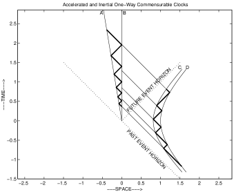
Figure 11: One-way commensurability between inertially expanding clock AB and accelerated clock BC, each containing its pulse bouncing back and forth. Depicted in this diagram is a sequence of 5 high intensity pulses coming from A and impinging on B which are matched by a sequence of 4 low intensity pulses coming across the event horizon from C. The ratio $m/n=5/4$ is the ticking rate of AB normalized to that of CD. The fact that this ratio stays constant throughout the history of the two clocks makes them one-way commensurable.

Commensurability is a more basic property than the property of clocks being synchronized. Before one tries to synchronize two clocks, one must first ascertain that they are commensurable.

Furthermore, two commensurable clocks cannot be synchronized unless there is a two-way interaction between them. In the context of an inertially expanding or an accelerated coordinate frame (Figure 9 or 10) such an interaction consists of a radar (to and fro) signal between each pair of clocks, say AB and CD as in Figures 7 or 8. Such a radar signal accommodates a two-way transfer of time: AB transmits its tick number to CD, and CD sends via the return pulse its own tick number back to AB. With this mutual knowledge the two clocks can be relabelled, if necessary, to give synchronized time.

However, if there is an event horizon between clocks AB and CD, then qualitatively new considerations enter.

On one hand, at most only a one-way transfer of time is possible. The establishment of a time synchronous to both of them is out of the question.

On the other hand, that event horizon brings with it a pleasant surprise: an accelerated clock and an inertially expanding clock, which at first sight seem to be incommensurable, are in fact commensurable when there is an event horizon between them. In particular one clock can (via sympathetic resonance) exert a one-way control over the other. Here is why:

As one can see from Figure 1 there is an event horizon that separates the clocks in spacetime sector $I$ from those in spacetime sector $F$. But the problem with taking advantage of a one-way transfer of time from CD in $I$ to AB in $F$ seems to be that the clock in $I$ is accelerated while the one in $F$ is inertially expanding. At first sight there seems to be no way that the two are commensurable as defined on page 7 in section IV.2. One must note, however, that that definition was based on a two-way transfer of time (“AB is radar-visible to CD”). This was necessary. Indeed, the definition of boost-invariant sector $I$ as well as $F$ (“equivalence classes of geometrical clocks that can be synchronized”) depended on it.

To accommodate the context of an event horizon as a one-way membrane between clocks AB and CD, we enlarge the concept “commensurability” by defining the concept “one-way commensurability”. This is done by dropping the requirement that radar units B and C be in two-way contact, and by saying that one-way contact, say from C to B, is good enough. The result of doing this is illustrated in Figure 11.

Accelerated clock CD moves along the line of sight of inertially expanding clock AB. This clock is characterized by Doppler shift factor $k_{AB}$. Clock CD, whose radar units are accelerated with constant accelerations $1/\xi_{C}$ and $1/\xi_{D}$ to the right, is characterized by the pseudo-gravitational frequency shift factor

$$k_{CD}=\frac{\xi_{D}}{\xi_{C}}$$

between them. As shown in Figure 11, clock CD sends pulses on a one-way journey to AB. There are no return pulses. Nevertheless, one can compare a sequence of $a$ pulses at B from A with a matched sequence of $c$ pulses from CD. The result is

$$\frac{a}{c}=\frac{(1/\log k_{AB})}{(1/\log k_{CD})}~{}.$$ (35)

This is the ticking rate of inertial clock AB normalized relative to accelerated clock CD. This ticking rate is a constant independent of the starting time of the two matched pulse sequences. Consequently, inertial clock AB is one-way commensurable with accelerated clock BC.

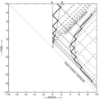
Figure 12: One-way transfer of time from clock CD to clock AB. This transfer is achieved by the ticking of CD causing sympathetic tickings in clock AB. This process is brought about by e.m. pulses travelling from CD across the future event horizon to AB (solid thin 45^∘ lines). They strike B at precisely the same rate and with the same phase as AB’s clock pulse (heavy zigzag line) bouncing repeatedly off B.

Equation (35) is a remarkable result for a number of reasons. First of all, there is its constancy. Contrast this with the tickings of the comoving atomic clocks at radar units B, which is floating freely, and C, which is accelerated. They yield

$$\frac{\textrm{(\# of ticks of atomic clock C but observed at B)}}{\textrm{(\# of ticks of atomic clock B)}}~{},$$

a corresponding rate which is a Doppler chirp towards the red as seen by a physicist comoving with the free-float atomic clock at B. By contrast, the constancy of Eq.(35) expresses the fact that the slowdown in the proper ticking rate of geometrical clock AB compensates precisely for the slowdown in the proper rate of pulses arriving at B from C.

Second, if $n/m=1$, i.e.

$$k_{AB}=k_{CD}~{},$$ (36)

then the process of transferring a train of clock pulses from across its future event horizon to clock AB (“one way transfer of time”) is a process of tickings in cavity CD bringing about sympathetic tickings in cavity AB. The implementation of this transfer is depicted in Figure 12. Thus, following the discussion in Section VI, one concludes that, even though CD is accelerated while AB is expanding inertially, (i) the two cavities are identically constructed from perspective of their normal mode spectra, and that (ii) AB and CD are ticking at the same rate as measured at B.

VIII TRANSFER OF RADAR DATA ACROSS AN EVENT HORIZON

Third, if clock CD controls the emission and reception of radar pulses to locate a scattering event in $I$ (filled circle in Figure 13), then upon being transferred to AB, these pulses can be used by AB to reconstruct an image of that event’s location in $F$ (unfilled circle in Figure 13). By applying this reconstruction to scattering events lying on, say, a time-like hyperbola in $I$, (dashed curve in Figure 13), one finds that its image in $F$ is a straight line in $F$ (dashed line in Figure 13). Similarly, a spacelike straight line of simultaneity gets reconstructed as a spacelike hyperbola of simultaneity in F.

Mathematically this reconstruction assumes its simples form when expressed in terms of the null coordinates

$$U=t-z$$

$$V=t+z$$

of Figure 1:

$$I \longrightarrow F$$

$$\left(\begin{array}[]{c}\textrm{Scattering}\\ \textrm{event in }I\end{array}\right):~{}(U_{I},V_{I}) \sim\!\rightarrow \left(\begin{array}[]{c}\textrm{Image of}\\ \textrm{scattering}\\ \textrm{event in }F\end{array}\right):~{}(U_{F},V_{F})=\left(\frac{b^{2}}{-U_{I}},V_{I}\right)$$

$$(\textrm{hyperbola in }I):~{}U_{I}V_{I}=const. \longrightarrow \left(\begin{array}[]{c}\textrm{Straight}\\ \textrm{line in }F\end{array}\right):~{}\frac{V_{F}}{U_{F}}=\frac{-const.}{b^{2}}$$

$$\left(\begin{array}[]{c}\textrm{Straight}\\ \textrm{line in }I\end{array}\right):~{}\frac{V_{I}}{U_{I}}=const. \longrightarrow (\textrm{hyperbola in }F):~{}U_{F}V_{F}=-b^{2}\times const.$$

Physically this reconstruction is based entirely on $1/b$, the acceleration of radar unit C of clock CD, and Eq.(36), the common frequency shift factor, which is best expressed in terms of the change in the boost coordinate $\tau$,

$$e^{\Delta\tau}\equiv k_{AB}=k_{CD}~{}.$$

Let

$$n_{2}=n+m$$

$$n_{1}=n-m$$

be the integer-valued radar coordinate of a scattering event located by CD in $I$. Then that event is related to its image in $F$ by

$$I \longrightarrow F$$

$$(t_{I},z_{I})=be^{m\Delta\tau}(\sinh n\Delta\tau,\cosh n\Delta\tau) \sim\!\rightarrow (t_{F},z_{F})=be^{n\Delta\tau}(\cosh m\Delta\tau,\sinh m\Delta\tau)$$

This is the relationship between the solid and the hollow circled events in Figure 13.

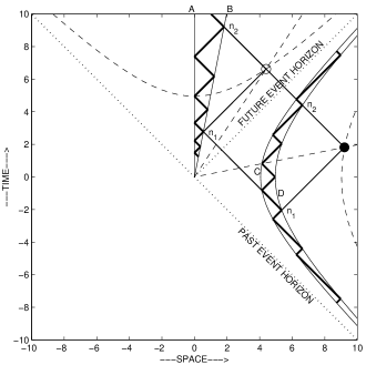
Figure 13: Transfer of radar coordinates from clock CD to clock AB. The heavy dot in $I$ gets mapped to the hollow dot in $F$. The radar coordinates of the event marked by the heavy black dot are the two clock pulses numbered $n_{1}$ and $n_{2}$ by accelerated clock CD. These two pulses cause CD to dispatch two pulses across its future event horizon. They are received by inertial clock AB where the numbering of its pulses is the same, namely, $n_{1}$ and $n_{2}$. These are also the radar coordinates of the encircled event (“hollow dot”) in $F$. If this and other such events lie along the straight dashed line in $F$, then a free-float physicist who watches AB knows that the scattering source in $I$ has the world line of the dashed hyperbola in $I$.

IX SUMMARY

The subject of this article is inertially expanding reference frames. The theme is their establishment as a one-way windows into uniformly and linearly accelerated reference frames. To execute this task, this article constructs both kinds of frames using the basic properties of Doppler radar and pulse radar and then points out a radar-generated mapping between the two frames.

The construction requires three ingredients. First one constructs “Fourier-compatible” geometrical clocks. Each one is characterized by a single number, the frequency shift factor between the moving ends of a one-dimensional moving cavity that traps an e.m. pulse. Its bouncing action provides the ticking of the clock.

Second one introduces geometrical clocks. In general, the ticking rates of these clocks are non-uniform relative to an atomic clock comoving with one end of the cavity, or the other. Thus the necessity of comparing one geometrical clock with another is fulfilled by considering the ratio of theses rates. This leads to the concept “commensurability” as applied to geometrical clocks. They are commensurable whenever one can choose one of them as a representative with its pair of properties (separation between successive ticks and separation between cavity ends) serving as a standard: the properties of all other clocks can be related to it numerically. Thus “commensurability” is a relation which implies and is implied by a standard of measurement. Moreover, “commensurability” is an equivalence relation. It divides clocks into mutually exclusive sets, which in mathematics are called equivalence classes and in physics are called reference frames, accelerated ($I$ or $II$ as in Figure 1) or inertially expanding ($F$ or $P$ as in Figure 1).

It is valuable to take note of the importance of commensurability as a general concept and as a special concept when applied to geometrical clocks in particular. It is the connecting link between nature (i.e. reality, existence) and the observer’s mind. This is because the observer can choose one of these clocks as a standard to which he can quantitatively relate all others (by taking ratios). Then, by referring to merely a single representative clock the observer can grasp the corresponding equivalence class of all possible commensurable clocks, a particular spacetime coordinate frame (accelerated or inertially expanding).

Without a measurement process of some sort, there would not be a commensurability criterion, there would not be an equivalence relation, hence no equivalence class, i.e. no concept. The concept of time and of place consists of the set of measurement results which the observer obtains when he relates the tickings and the size of his standard clock to any event occurring in his reference frame. Establishing these relations is what he means by measuring (the time and place of) these events.

The third ingredient consists of specifying some sort of measurement process. Just as a one-dimensional array of calibrated graduation marks on a measuring rod facilitates measuring the length of any specific object, so a lattice of calibrated graduation events in a spacetime coordinate frame facilitates measuring the time and position of any specific event. The calibration process can be performed by the radar method, which is based on having a single standard clock control the emission and the reception of radar pulses, or by the common (non-radar) method, which is based on counting synchronized identically constructed clocks (i.e. copies of the clock chosen as a standard) and their ticks. Even though the equivalence of these two methods extends to accelerated as well as inertially exspanding clocks, the introduction of radar does not make identically constructed clocks obsolete or useless.

On the contrary. Suppose one applies the essential aspect of being “identically constructed” to two clocks separated by an event horizon between them. “Identical construction” means that, even though one clock is accelerated while the other is inertially expanding, their cavities have identical eigenfrequency spectra, and that, as a consequence, the timing pulses emitted by the accelerated clock cause the inertially expanding clock to tick in perfect synchrony with their arrival at this clock.

Thus the first useful aspect of two “identically constructed” clocks, one accelerated the other inertially expanding, is that they lend themselves to being (one-way) synchronized even though they are separated by an event horizon.

The second and more important aspect is that a physicist in the inertially expanding frame can “look” into the accelerated frame on the other side of the event horizon and “see” the spacetime trajectories of sources in that frame. This is because the two clocks serve to (one-way) transfer radar images across the event horizon. The elements (pixels) of a radar image are in the form of the amplitudes of the pulses reflected by a scatterer located in the frame of the accelerated clock. Taking advantage of its transponder capability, the accelerated clock forwards these pulses to the identically constructed inertially expanding clock. There the pulses are used to reconstruct a spacetime image of what the accelerated clock sees. For example, suppose the radar controlled by this clock measures that a localized scatterer has the history of a hyperbolic world line in boost-invariant sector $I$. Once the pixels of this radar image have been sent across the event horizon, the inertially expanding clock reconstructs them into a straight timelike line in boost-invariant sector $F$. As a second example, the pixels of a linear array of simultaneous scattering events in $I$, upon transmission across the event horizon, get reconstructed as a spacelike hyperbola in $F$.

Thus, by using an accelerated and an inertially expanding clock which are “identically constructed”, an inertial observer can verify by radar whether the dipole source in the augmented Larmor formula is accelerated in a uniform and linear way.

X THREE CONCLUSIONS

The augmented Larmor formula, Eq.(1), is a mathematical relation between a dipole source located in an accelerated frame and an integral of the Poynting vector observed in the inertially expanding reference frame, a relation between cause and effect.

The Poynting integral is a quantity quadratic in the e.m. field $\{\vec{E}(x),\vec{B}(x)\}$. Recall that to determine this quantity experimentally and to validate it as a Maxwell field requires two distinct measuring processes. The first one measures the magnitude and the direction of the e.m. field quantities. This is usually done with an antenna, a radio receiver, and a volt meter. The second one ascertains the place and the time of this receiving antenna in relation to the dipole source. This is usually done optically. The physicist illuminates his receiving antenna with optical radiation.

The experimental determination of the e.m. field quantities consists then of establishing a quantitative relation between the results of the two measuring processes, the optical measurements and those obtained with the receiving antenna. The augmented Larmor formula, Eq.(1), is an example of such a relation. The independent variable $\tau$ is measured optically. The dependent variable (flow of radiant energy into the direction of acceleration) is measured with the receiving antenna. The $\tau$-measurements consist of identifying the relationship between observation events in $F$ and the tickings of the expanding reference clock AB in Figure 9. This clock also serves to make the $\tau$-measurements of the source events in $I$, but only after their coordinates have been transferred (by means of the “radar map”) from $I$ to $F$ as illustrated in Figure 13.

An obvious feature of Eq.(1) is that it differs from the standard Larmor formula by a significant contribution. However, one should not conclude from this that there is any contradiction with established knowledge. This is because the prominent assumption that went into the derivation of Eq.(1) is that the measurement of the e.m. Poynting integral is done in an inertially expanding coordinate frame. By contrast, the standard Larmor radiation formula assumes that the measurement of the e.m. Poynting vector is done in a free-float (“inertial”, “Lorentz”) coordinate frame.

The difference between the standard and the augmented Larmor formula goes with the difference between a free-float and an inertially expanding reference frame. These two frames are incommensurable. An attempt to evade this difference by, for example, invoking a coordinate transformation between Minkowski and boost coordinates or by resorting to “covariance” would be like trying to transform apples into oranges. The two coordinate frames reveal entirely different aspects of nature, and the radiation from an e.m. source is one of them.

X.1 Boost Coordinates as Physical and Nonarbitrary

What one should conclude is the opposite of what some authors have asserted in the past. For example, they claimed that “$\cdots$ the coordinates that we use [for computation] are arbitrary and have no physical meaning” or “It is the very gist of relativity that anybody may use any frame [in his computations].” Without delving into the logical fallacies underlying these claims, one should be aware of their unfortunate consequences. They tend to discourage attempts to understand natural processes whose very existence and identity one learns through measurements and computations based on nonarbitrary coordinate frames. The identification of radiation from bodies with extreme acceleration is a case in point. For these, two complementary frames are necessary: an accelerated frame to accommodate the source (boost-invariant sector $I$ and/or $II$) and the corresponding expanding inertial frame (boost-invariant sector $F$) to observe the information carried by the radiation coming from this source. These frames are physically and geometrically distinct from static inertial frames. They also provide the logical connecting link between the concepts and the perceptual manifestations (via measurements) of these radiation processes. Without these frames the concepts would not be concepts but mere floating abstractions.

X.2 Conjoint Boost-Invariant Frames as an Arena for Scattering Processes

The most prominent feature of radiation from a body with extreme acceleration is the kinematics necessary for its observation. One needs two coordinate frames: one for the accelerated source, the other for the inertial observer. It is vital that these two frames be aligned properly (as in Figure 12) so that the geometrical clock of one frame is (one-way) commensurable with the clock of the other. This commensurability locks the two frames into a conjoint coordinate frame with an event horizon between them.

This conjointness opens vistas which are closed to the familiar inertial frames with their respective lattice work of free-float clocks and rods Taylor and Wheeler (1992). An obvious example is the measurement of the acceleration radiation scattered by a dipole oscillator as it accelerates through the e.m. field in its Minkowski vacuum state. The augmented Larmor formula applied to this oscillator yields the result that it scatters black body radiation with 100% spectral fidelity relative to the inertially expanding reference frame.

X.3 Boost Coordinate Frame as a Valid Coordinate Frame in Quantum Field Theory

The consistent use of geometrical clocks puts constraints on the mathematical formulation of waves propagating in the inertially expanding coordinate frame $F$. In this frame, a standard inertially expanding clock AB characterized by Doppler frequency shift factor Eq.(33),

$$k_{AB}=e^{(\tau_{B}-\tau_{A})}\equiv e^{\Delta\tau},$$

generates pulses whose null histories as depicted in Figure 2 are

$$\xi e^{\tau} = be^{n_{2}\Delta\tau}~{}~{}~{}~{}~{}n_{2}=0,\pm 1,\cdots~{}~{}$$ (40)

$$\xi e^{-\tau} = be^{n_{1}\Delta\tau}~{}~{}~{}~{}~{}n_{1}=0,\pm 1,\cdots~{}~{}.$$ (41)

The graduation events calibrated by this geometrical clock yield therefore the following discrete boost coordinates

$$\xi = be^{N\Delta\tau},~{}~{}~{}~{}~{}N=\frac{n_{2}+n_{1}}{2}$$ (42)

$$e^{\tau} = e^{M\Delta\tau},~{}~{}~{}~{}~{}M=\frac{n_{2}-n_{1}}{2}~{}.$$ (43)

As illustrated in Figure 9 and discussed in Section V.2, they are the boost coordinates of the $M$th identically constructed clock with its $N$th ticking event.

In a paper some time ago Padmanabhan (1990) Padmanabhan considered the evolution of normal modes of the wave equation $(\Box-m^{2})\psi=0$ in the boot-invariant coordinate frame $F$.

Starting with a normal mode characterized by positive boost frequency in the distant past of $F$, he observed that this mode, in compliance with the wave equation, evolved into a mixture of positive and negative frequencies in the distant future of $F$. From the viewpoint of quantum theory such a mixture indicates a production of particles and antiparticles. This formulation of waves propagating in $F$ therefore leads to the mathematical prediction that, in analogy with Parker’s particle-antiparticle creation mechanism Parker (1982) due to a time-dependent gravitational field, particles and antiparticles get created because of the time-dependence of the boost-invariant metric, Eq.(44), in $F$.

This prediction is, of course, invalid. It contradicts the absence of any such particle creation in flat spacetime, where there is no gravitational field. But the procedure leading to this contradiction, Padmanbhan points out, is mathematically sound and completely conventional [our emphasis]. In order to avoid this contradiction he proposes that, within the context of quantum theory (i.e. particle-antiparticle production), one exclude Bondi and Rindler’s spacetime coordinatization as physically inadmissible.

However happy one must be about the scrutiny to which that coordinatization has been subjected, one must not forget that Padmanabhan’s procedure leading to to the above contradiction is far from “completely conventional”. In fact, it violates the central principle of measurement (Section III): “once a standard of time has been chosen, it becomes immutable for all subsequent measurements”. Here is how the violation occurs:

In spacetime sector $F$, where the invariant interval has the form

$$ds^{2}=-d\xi^{2}+\xi^{2}d\tau^{2}+dy^{2}+dx^{2}~{},$$ (44)

the normal modes of the wave equation $(\Box-m^{2})\psi=0$ have the form

$$\psi=\psi_{k}(\xi,\tau)e^{i(k_{y}y+k_{x}x)}~{},$$

Where $\psi_{k}(\xi,\tau)$ satisfies

$$\left[\frac{1}{\xi}\frac{\partial}{\partial\xi}\xi\frac{\partial}{\partial\xi}-\frac{1}{\xi^{2}}\frac{\partial^{2}}{\partial\tau^{2}}+k^{2}\right]\psi_{k}(\xi,\tau)=0$$

with $k^{2}\equiv k_{y}^{2}+k_{x}^{2}+m^{2}$. A typical normal mode has the form

$$\psi = J_{-i\omega}(k\xi)e^{i\omega\tau}e^{i(k_{y}y+k_{x}x)}$$ (45)

$$= \frac{1}{2}\left[H_{-i\omega}^{(1)}(k\xi)+H_{-i\omega}^{(2)}(k\xi)\right]e^{i\omega\tau}e^{i(k_{y}y+k_{x}x)}$$ (46)

Measuring its field consists of sampling it at the events (time $\xi$ and location $\tau$) controlled and calibrated by a set of identically constructed clocks. If these clocks are inertially expanding clocks as in Figure 9, then the sampling events are given by Eqs.(42)-(43), and the sampled field values are

$$\psi = J_{-i\omega}(kbe^{N\Delta\tau})e^{i\omega M\Delta\tau}e^{i(k_{y}y+k_{x}x)}$$

$$\propto (kb)^{-i\omega}e^{-i\omega(N\Delta\tau)}e^{i\omega M\Delta\tau}e^{i(k_{y}y+k_{x}x)}\textrm{ as }N\to-\infty$$

If the samples are are close enough (i.e. $\Delta\tau$ small enough), then, using Shannon’s sampling theorem, one reconstructs the field from the sampled values of its field.

Note that even though this clock-controlled sampling measurement reconstructs the the field uniquely in the distant past ($N\to-\infty$) of $F$, it is clear that this is not the case in the distant future ($N\to\infty$). Regardless how small one makes the separation between the sampling events in the asymptotic past, in the asymptotic future the inertially expanding clocks tick at such a slow rate (compared to any atomic clock) that there is no possibility of reconstructing the field from the sampling measurements. Indeed, in the distant future ($\xi=be^{N\Delta\tau}\to\infty$), the field, Eq.(46),

$$\psi\approx\frac{1}{2}\sqrt{\frac{2}{\pi k\xi}} \!\!\!\!\!\!\left[e^{-\pi\omega/2}e^{i(k\xi-\pi/4)}+e^{\pi\omega/2}e^{-i(k\xi-\pi/4)}\right]$$

$$\times~{}e^{i\omega\tau}e^{i(k_{y}y+k_{x}x)}$$

oscillates at a steady rate as a function of (atomic=proper) $\xi$. But the sampling events, as one can see readily from Figure 9, are so sparsely spaced as $N\to\infty$ that there is more than one oscillation between them. Consequently, reconstruction becomes non-unique and hence out of the question. In particular, sampling measurements controlled by an inertially expanding clock are incapable of distinguishing normal modes traveling into opposite directions, to say nothing about identifying their oscillation frequencies in the distant future of $F$.

Would an atomic clock do better? The answer is yes. But only for sampling measurements made in the distant future ($\xi=be^{N\Delta\tau}\to\infty$). For the distant past ($N\to\infty,~{}\xi=be^{N\Delta\tau}\to 0$) atomic clocks are just as useless as inertially expanding clocks are for the distant future: the clocks simply do not sample the field fast enough to identify its boost oscillation frequency.

Thus neither atomic clocks nor inertially expanding clocks can give measurements which identify the nature of the field in both the asymptotic past and the asymptotic future of $F$. One can measure the field in one or the other but not both.

A claim that in boost-invariant sector $F$ a pure positive boost frequency ($\omega$) mode evolves into a superposition of positive and negative inertial frequency ($\pm k$) modes is wrong. This is because it makes the tacit assumption that one change inertially expanding to static atomic clocks in midstream. Making such a change would go counter to the central principle of measurement (Section III): “once a standard has been chosen it becomes immutable for all subsequent measurements”. Violating it would make a standard into a non-standard.

But a standard is precisely what is needed, otherwise there would be no way of assigning a frequency and a direction of propagation to normal modes, the key ingredients to mode amplification and hence to particle creation as formulated in quantum field theory. Put differently, an assertion that a mode having a positive frequency evolve mathematically into a mixture of positive and negative frequency modes must be accompanied by a specification of a (system of commensurable) standard clock(s).

It is evident that in sector $F$ no such standard exists. Consequently, one is not entitled to claim that mathematical analysis of free fields in that sector predicts the creation of particles.

XI ACKNOWLEDGEMENTS

The author appreciates useful conversations about laser physics with Mark Walker and Linn Van Woerkom.

References

- Misner et al. (1973a) C. W. Misner, K. S. Thorne, and J. A. Wheeler, GRAVITATION (W.H. Freeman and Company, San Francisco, 1973a), chap. 6.3, pp. 168–169.
- Misner et al. (1973b) C. W. Misner, K. S. Thorne, and J. A. Wheeler, GRAVITATION (W.H. Freeman and Company, San Francisco, 1973b), chap. 6.6, pp. 172–173.
- Gerlach (2001) U. H. Gerlach, Physical Review D 64, 105004 (2001), eprint [http://arXiv.org/abs/gr-qc]gr-qc/0110048, URL http://www.math.ohio-state.edu/~gerlach.
- Trautman et al. (1965) A. Trautman, F. Pirani, and H. Bondi, Lectures on GENERAL RELATIVITY (Prentice-Hall, Inc., Englewood Cliffs, N.J., 1965), vol. 1 of Brandeis Summer Institute in Theoretical Physics, 1964, pp. 377–406.
- Rindler (1966) W. Rindler, American Journal of Physics 34, 1174 (1966).
- Taylor and Wheeler (1992) E. F. Taylor and J. A. Wheeler, SPACETIME PHYSICS (W.H. Freeman and Company, San Francisco, 1992), chap. 2.6, pp. 37–39, 2nd ed.
- Binswanger and Peikoff (1990) H. Binswanger and L. Peikoff, eds., Introduction to Objectivist Epistemology (Meridian, a division of Penguin Books USA Inc., New York, 1990), 2nd ed.
- Peikoff (1993) L. Peikoff, OBJECTIVISM: The Philosophy of Ayn Rand (Meridian, a division of Penguin Books USA Inc., New York, 1993).
- Udem et al. (2002) T. Udem, R. Holwarth, and T. Haensch, Nature 416, 233 (2002).
- Chiu and Hoffman (1963) H.-Y. Chiu and W. F. Hoffman, GRAVITATION AND RELATIVITY (W.A. Benjamin, Inc., New York, N.Y., 1963).
- Einstein (1961) A. Einstein, RELATIVITY: The Special and the General Theory (Crown Publishers, Inc., New York, 1961).
- Wolf (1980) H. Wolf, ed., Some Strangeness in Proportion (Addison-Wesley Publishing Company, Inc., Reading, Mass., 1980), p. 285.
- Schroedinger (1956) E. Schroedinger, EXPANDING UNIVERSES (Cambridge University Press, New York, 1956), p. 20.
- Padmanabhan (1990) T. Padmanabhan, Phys. Rev. Lett. 64, 2471 (1990).
- Parker (1982) L. Parker, Fundamentals of Cosmic Physics 7, 201 (1982).