Equatorial circular orbits in the Kerr–de Sitter spacetimes

Abstract

Equatorial motion of test particles in Kerr–de Sitter spacetimes is considered. Circular orbits are determined, their properties are discussed for both black-hole and naked-singularity spacetimes, and their relevance for thin accretion disks is established. The circular orbits constitute two families that coalesce at the so-called static radius. The orientation of the motion along the circular orbits is, in accordance with case of asymptotically flat Kerr spacetimes, defined by relating the motion to the locally nonrotating frames. The minus-family orbits are all counterrotating, while the plus-family orbits are usually corotating relative to these frames. However, the plus-family orbits become counterrotating in the vicinity of the static radius in all Kerr–de Sitter spacetimes, and they become counterrotating in the vicinity of the ring singularity in Kerr–de Sitter naked-singularity spacetimes with a low enough rotational parameter. In such spacetimes, the efficiency of the conversion of the rest energy into heat energy in the geometrically thin plus-family accretion disks can reach extremely high values exceeding the efficiency of the annihilation process. The transformation of a Kerr–de Sitter naked singularity into an extreme black hole due to accretion in the thin disks is briefly discussed for both the plus-family and minus-family disks. It is shown that such a conversion leads to an abrupt instability of the innermost parts of the plus-family accretion disks that can have strong observational consequences.

I Introduction

It is commonly accepted that the energy sources of quasars and active galactic nuclei are accretion disks around central massive black holes Abr-Per:1997:CLAQG: ; Bla:1990:AGN: . The basic properties of geometrically thin accretion disks (with negligible pressure) are determined by the circular geodesic motion in the black-hole backgrounds Nov-Tho:1973:BlaHol: . The basic properties of geometrically thick disks are determined by the equilibrium configurations of a perfect fluid orbiting in the black-hole background; however, the geodesic structure of the background is relevant also for the properties of the thick disks Jar-Abr-Pac:1980:ACTAS: .

According to the cosmic censorship hypothesis Pen:1969:NUOC2: and the uniqueness theorems for black holes Car:1973:BlaHol: , the result of the gravitational collapse of a sufficiently massive rotating object is a rotating Kerr black hole, rather than a Kerr naked singularity; further, the laws of black-hole thermodynamics forbid conversion of black holes into a naked singularity. However, although the cosmic censorship is a very plausible hypothesis, there is some evidence against it. Naked singularities arise in various models of spherically symmetric collapse (e.g. Lak-Zan:1990:PHYSR4: ). In modeling the collapse of rotating stars, it was pointed out that, although mass shedding and gravitational radiation will reduce the angular momentum of the star during collapse, it will not in general be reduced to the value that corresponds to a Kerr black hole Mil-deFel:1985:ASTRJ2: .The 2D numerical models Nak-Ooh-Koj:1987:PROTP3: imply that a rotating, collapsing supermassive object will not always dissipate enough angular momentum to form a Kerr black hole, but a Kerr-like naked singularity has to be expected to develop from objects rotating rapidly enough. Candidates for the formation of naked Kerr geometry with a ring singularity from the collapse of rotating stars were found in the scenario of Char-Cla:1990:CLAQG: . The numerical models of the collapse of collisionless gas spheroids also results in strong candidates for the formation of naked singularities Sha-Teu:1992:PHYSR4: .

Because Penrose’s cosmic censorship hypothesis Pen:1969:NUOC2: is far from being proved, naked singularity spacetimes related to black-hole spacetimes with a nonzero charge and/or rotational parameter could still be considered conceivable models of quasars and active galactic nuclei and deserve some attention. Of particular interest are those effects that could distinguish a naked singularity from black holes.

Test particle motion and test fields were extensively studied for Kerr black-hole spacetimes Car:1968:PHYSREV: ; Bar-Pre-Teu:1972:ASTRJ2: ; Bar:1973:BlaHol: ; Ste-Wal:1973:SpringerTracts: ; Bic-Stu:1976:BULAI: ; Sha:1979:GENRG1: ; Con:1984:GENRG1: ; Dym:1986:SOVPU2: ; Bic-Stu-Bal:1989:BULAI: ; Bal-Bic-Stu:1989:BULAI: . Gravitational radiation of particles moving in the field of a Kerr black hole were discussed in Sai-Shi-Mae:1997:PHYSR4: ; the motion of spinning test particles was discussed in Sem:1999:MONNR: . For a detailed review see the books of Chandrasekhar Chan:1983:BlackHoles: and Frolov and Novikov Fro-Nov:1998:BlackHolePhys: . However, Kerr naked singularities were also studied widely. Their repulsive effects and causality-violating regions were investigated by de Felice and co-workers deFel:1975:ASTRA: ; deFel-Cal:1979:GENRG1: ; deFel-Bra:1988:CLAQG: , the equatorial circular geodesics and motion of spherical shell of incoherent dust were investigated in Stu:1980:BULAI: , the collimation effect of the region nearby the ring singularity was treated in Bic-Sem-Had:1993:MONNR: , and the motion of spinning test particles was discussed in Sem:1999:MONNR: . Chandrasekhar Chan:1983:BlackHoles: also devotes some attention to the effects of Kerr naked singularities, saying “considerable interest attaches to knowing the sort of things space-times with naked singularities are and whether there are any essential differences in the manifestations of space-times with singularities concealed behind event horizons.” We follow Chandrasekhar’s approach.

All recently available data from a wide variety of cosmological tests indicate convincingly that in the framework of the inflationary cosmology a nonzero, although very small, repulsive cosmological constant $\Lambda>0$ has to be invoked in order to explain the dynamics of the recent Universe Bah-etal:1999:SCIEN: ; Kol-Tur:1990:EarUni: . The presence of a repulsive cosmological constant changes substantially the asymptotic structure of the black-hole (or naked-singularity) backgrounds, as they become asymptotically de Sitter spacetimes, not flat spacetimes. In such spacetimes, an event horizon always exists behind which the geometry is dynamic; we call it a cosmological horizon. Therefore, it is relevant to clarify the influence of the repulsive cosmological constant on the astrophysically interesting properties of the black-hole or naked-singularity background. For these purposes, analysis of the geodesic motion of test particles and photons is among the most important techniques. (It could be noted that the optical reference geometry introduced by Abramowicz and co-workers Abr-Car-Las:1988:GENRG1: reflects in an illustrative and intuitive way some hidden properties of the geodesic motion Abr-Pra:1990:MONNR: ; Hle:2002:JB60: ; Stu-Hle:2000:CLAQG: .) Of particular interest are circular geodesics being relevant for the accretion disks.

Properties of the geodesic motion in the Schwarzschild–(anti-)de Sitter and Reissner–Nordström– (anti-)de Sitter spacetimes were discussed in Stu-Hle:1999:PHYSR4: ; Stu-Hle:2002:ACTPS2: . Properties of the circular orbits of test particles show that due to the presence of a repulsive cosmological constant  the thin disks have not only an inner edge determined (approximately) by the radius of the innermost stable circular orbit, but also an outer edge given by the radius of the outermost stable circular orbit, located nearby the so-called static radius, where the gravitational attraction of a black hole (naked singularity) is just compensated for by the cosmological repulsion.

A similar analysis of the equilibrium configurations of a perfect fluid orbiting the Schwarzschild–de Sitter black-hole backgrounds allowing the existence of stable circular orbits, which is a necessary condition for the existence of accretion disks, shows that also thick accretion disks have both the inner and outer edges located nearby the inner (outer) marginally bound circular geodesic. The accretion through the inner cusp and the outflow of matter through the outer cusp of the equilibrium configurations are driven by the Paczyński mechanism. It is a mechanical nonequilibrium process when the matter of the disk slightly overfills the critical equipotential surface with two cusps and thus violates the hydrostatic equilibrium Stu-Sla-Hle:2000:ASTRA: .

In the case of Reissner–Nordström–(anti-)de Sitter  backgrounds Stu-Hle:2002:ACTPS2: , the discussion has been enriched for the case of the naked-singularity spacetimes—it was shown that even two separated regions of stable circular orbits are allowed for the naked-singularity spacetimes with spacetime parameters appropriately chosen.

However, it is very important to understand the role of a nonzero cosmological constant in the astrophysically most relevant, rotating, Kerr backgrounds. Equatorial motion of photons has been studied extensively for Kerr–Newman–(anti-)de Sitter spacetimes describing both black holes and naked singularities and some unusual effects have been found (for details, see Stu-etal:1998:PHYSR4: ; Stu-Hle:2000:CLAQG: ). Here, attention will be focused on the circular equatorial motion of test particles in the Kerr–de Sitter backgrounds.

In Sec. II, the Kerr–de Sitter backgrounds are separated in the parameter space into black-hole and naked-singularity spacetimes. In Sec. III, the equations of the equatorial motion of test particles are presented. In Sec. IV, the constants of motion of the circular orbits are determined, and their properties are discussed. As in Kerr spacetimes, there exist two different sequences of the equatorial circular geodesics. We call them plus (minus-) family orbits. All minus-family orbits are counterrotating relative to the locally nonrotating frames (LNRF; for a definition of these frames see Bar:1973:BlaHol: ), while the plus-family orbits are mostly corotating, but in some regions are counterrotating relative to the LNRF. Only outside the outer horizon of the Kerr black holes are all the plus-family orbits corotating relative to the LNRF. On the other hand, in vicinity of the ring singularity of the Kerr naked singularities with rotational parameter low enough, the plus-family orbits become counterrotating relative to the LNRF Stu:1980:BULAI: . We shall see that in all Kerr–de Sitter spacetimes this happens nearby the so-called static radius, where the sequences of plus-family and minus-family orbits coalesce. [Note that in asymptotically flat Kerr spacetimes, the orbits corotating (counterrotating) relative to the LNRF also corotate (counterrotate) from the point of view of stationary observers at infinity. However, the last criterion cannot be used in the asymptotically de Sitter spacetimes under consideration.] In Sec. V, the properties of the circular orbits are discussed with attention focused on their relevance for thin accretion disks. Regions where the orbits of the plus-family are counterrotating relative to the LNRF are determined; further, it is established where these orbits could have a negative energy parameter. The efficiency of the accretion process in geometrically thin disks is determined. In Sec. VI, concluding remarks are presented.

II Kerr–de Sitter black-hole and naked-singularity spacetimes

In the standard Boyer-Lindquist coordinates ($t,r,\theta,\varphi$) and geometric units ($c=G=1$), the Kerr–(anti-)de Sitter geometry is given by the line element

$$\mbox{d}s^{2} = -\frac{\Delta_{r}}{I^{2}\rho^{2}}(\mbox{d}t-a\sin^{2}\theta\mbox{d}\varphi)^{2}$$ (1)

$$+\frac{\Delta_{\theta}\sin^{2}\theta}{I^{2}\rho^{2}}\left[a\mbox{d}t-\left(r^{2}+a^{2}\right)\mbox{d}\varphi\right]^{2}$$

$$+\frac{\rho^{2}}{\Delta_{r}}\mbox{d}r^{2}+\frac{\rho^{2}}{\Delta_{\theta}}\mbox{d}\theta^{2},$$

where

$$\Delta_{r} = -\frac{1}{3}\Lambda r^{2}\left(r^{2}+a^{2}\right)+r^{2}-2Mr+a^{2},$$ (2)

$$\Delta_{\theta} = 1+\frac{1}{3}\Lambda a^{2}\cos^{2}\theta,$$ (3)

$$I = 1+\frac{1}{3}\Lambda a^{2},$$ (4)

$$\rho^{2} = r^{2}+a^{2}\cos^{2}\theta.$$ (5)

The parameters of the spacetime are mass ($M$), specific angular momentum ($a$), and cosmological constant ($\Lambda$). It is convenient to introduce a dimensionless cosmological parameter

$$y=\frac{1}{3}\Lambda M^{2}.$$ (6)

For simplicity, we put $M=1$ hereafter. Equivalently, also the coordinates $t,\ r$, the line element $\mbox{d}s$, and the parameter of the spacetime $a$ are expressed in units of $M$ and become dimensionless.

For $y<0$ corresponding to the attractive cosmological constant, the line element (1) describes a Kerr–anti–de Sitter geometry. Here we focus our attention on the case $y>0$ corresponding to the repulsive cosmological constant, when Eq. (1) describes a Kerr–de Sitter spacetime.

The event horizons of the spacetime are given by the pseudosingularities of the line element (1), determined by the condition $\Delta_{r}=0$. The loci of the event horizons are determined by the relation

$$a^{2}=a^{2}_{h}(r;y)\equiv\frac{r^{2}-2r-yr^{4}}{yr^{2}-1}.$$ (7)

The asymptotic behavior of the function $a^{2}_{h}(r;y)$ is given by $a^{2}_{h}(r\rightarrow 0,y)\rightarrow 0$, $a^{2}_{h}(r\rightarrow\infty,y)\rightarrow-\infty$. For $y=0$, the function $a^{2}_{h}(r)=2r-r^{2}$ determines loci of the horizons of Kerr black holes. The divergent points of $a^{2}_{h}(r;y)$ are determined by

$$y=y_{d(h)}(r)\equiv\frac{1}{r^{2}},$$ (8)

its zero points are given by

$$y=y_{z(h)}(r)\equiv\frac{r-2}{r^{3}},$$ (9)

and its local extrema are determined by the relation

$$y=y_{\mathop{\rm e}(h)\pm}(r)\equiv\frac{2r+1\pm\sqrt{8r+1}}{2r^{3}}.$$ (10)

The functions $y_{d(h)}(r)$, $y_{z(h)}(r)$, and $y_{\mathop{\rm e}(h)\pm}(r)$ are illustrated in Fig. 1.

Figure 1: Functions $y_{e(h)-}(r)$ (solid curve), $y_{z(h)}(r)$ (dashed curve), $y_{d(h)}(r)$ (dash-dotted curve), and $y_{e(h)+}(r)$ (dotted curve) characterizing the properties of the function $a^{2}_{h}(r;y)$ determining the horizons of Kerr–de Sitter spacetimes. The maximum of $y_{e(h)-}(r)$ corresponds to the critical value of the cosmological parameter $y_{c(KdS)}\doteq 0.05924$ for which the function $a^{2}_{h}(r;y)$ has an inflex point (and no extrema). Any Kerr–de Sitter spacetime with $y>y_{c(KdS)}$ is of naked-singularity type containing only a cosmological horizon. The function $y_{z(h)}(r)$ determines the horizons of the Schwarzschild–de Sitter spacetimes and its maximum $y_{c(SdS)}=1/27$ corresponds to the limiting value for the existence of Schwarzschild–de Sitter black holes.

The function $y_{\mathop{\rm e}(h)-}(r)$ has its maximum at $r_{\rm crit}=(3+2\sqrt{3})/4$, where the value of the cosmological parameter takes a critical value

$$y_{c(KdS)}=\frac{16}{(3+2\sqrt{3})^{3}}\doteq 0,05924;$$ (11)

for $y>y_{c(KdS)}$, only naked-singularity backgrounds exist for $a^{2}>0$. A common point of the functions $y_{z(h)}(r)$ and $y_{e(h)-}(r)$ is located at $r=3$, where is the maximum of $y_{z(h)}(r)$ taking a critical value

$$y_{c(SdS)}=\frac{1}{27}\doteq 0.03704,$$ (12)

which is the limiting value for the existence of Schwarzschild–de Sitter black holes Stu-Hle:1999:PHYSR4: . In Reissner–Nordström–de Sitter spacetimes, the critical value of the cosmological parameter limiting the existence of black-hole spacetimes is Stu-Hle:2002:ACTPS2:

$$y_{c(RNdS)}=\frac{2}{27}\doteq 0.07407.$$

If $y=y_{c(KdS)}$, the function $a^{2}_{h}(r;y)$ has an inflex point at $r=r_{\rm crit}$, corresponding to a critical value of the rotation parameter of Kerr–de Sitter spacetimes:

$$a^{2}_{\rm crit}=\frac{3}{16}(3+2\sqrt{3})\doteq 1,21202.$$ (13)

Kerr–de Sitter black holes can exist for $a^{2}<a^{2}_{\rm crit}$ only, while Kerr–de Sitter naked singularities can exist for both $a^{2}<a^{2}_{\rm crit}$ and $a^{2}>a^{2}_{\rm crit}$.

For $y>0$, the function $y_{\mathop{\rm e}(h)-}(r)$ determines two local extrema of $a^{2}_{h}(r;y)$ at $y<y_{c(KdS)}$, denoted as $a^{2}_{\mathop{\rm max}(h)}(r_{1},y)$, $a^{2}_{\mathop{\rm min}(h)}(r_{2},y)$, with $r_{1}<r_{2}$. If $y<y_{c(SdS)}$, $a^{2}_{\mathop{\rm min}(h)}(r_{2},y)<0$, and the minimum is unphysical. The function $a^{2}_{h}(r)$ diverges at $r_{d}=1/\sqrt{y}$, and it is discontinuous there. The function $y_{\mathop{\rm e}(h)+}(r)$ determines a maximum of $a^{2}_{h}(r;y)$ at a negative value of $a^{2}$ which is, therefore, physically irrelevant [see Fig. 2 giving typical behavior of $a^{2}_{h}(r;y)$].

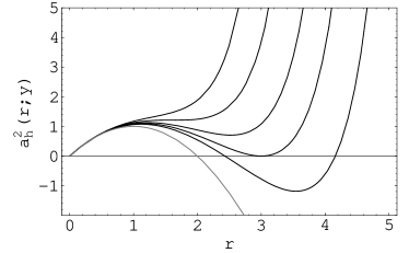
Figure 2: Horizons of Kerr–de Sitter spacetimes. They are given for five typical values of the cosmological parameter $y$ by the function $a^{2}_{h}(r;y)$. For $y>y_{c(KdS)}\doteq 0.05924\ (y=0.08)$ the function has no local extrema and only naked-singularity spacetimes are allowed (the only horizon is the cosmological horizon). For $y=y_{c(KdS)}$, the function has an inflex point where the black-hole and the cosmological horizons coincide. For $y_{c(SdS)}=1/27<y<y_{c(KdS)}\ (y=0.045)$ the function has two local extrema in positive values and the black-hole spacetimes exist for $a^{2}$ between those extrema. For $y=y_{c(SdS)}$ the local minimum resides on the axis $a^{2}=0$. The ciritical value $y_{c(SdS)}$ represents the limiting value of cosmological parameter for which the Schwarzschild–de Sitter black holes can exist; the Kerr–de Sitter black holes again exist for $a^{2}$ between those extrema. For $0<y<y_{c(SdS)}\ (y=0.03)$ the local minimum resides in the nonphysical region $a^{2}<0$ and the black holes exist for $a^{2}$ up to the local maximum. For completeness, we present the gray curve determining horizons of the Kerr $(y=0)$ black holes. In all cases, the local extrema correspond to the extreme black holes.

If $0<y<y_{c(SdS)}$, black-hole spacetimes exist for $a^{2}\leq a^{2}_{\mathop{\rm max}(h)}(y)$, and naked-singularity spacetimes exist for $a^{2}>a^{2}_{\mathop{\rm max}(h)}(y)$. If $y_{c(SdS)}<y\leq y_{c(KdS)}$, black-hole spacetimes exist for $a^{2}_{\mathop{\rm min}(h)}(y)\leq a^{2}\leq a^{2}_{\mathop{\rm max}(h)}(y)$, while naked-singularity spacetimes exist for $a^{2}<a^{2}_{\mathop{\rm min}(h)}(y)$ and $a^{2}>a^{2}_{\mathop{\rm max}(h)}(y)$. The functions $a^{2}_{\mathop{\rm min}(h)}(y)$, $a^{2}_{\mathop{\rm max}(h)}(y)$ are implicitly given by Eqs. (7) and (10); the separation of Kerr–de Sitter black-hole and naked-singularity spacetimes in the parameter space $y$–$a^{2}$ is shown in Fig. 3. In black-hole spacetimes, there are two black-hole horizons and the cosmological horizon, with $r_{h-}<r_{h+}<r_{c}$. In naked-singularity spacetimes, there is the cosmological horizon $r_{c}$ only.

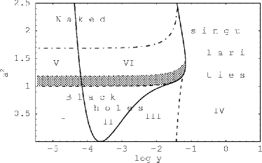
Figure 3: Classification of Kerr–de Sitter spacetimes. The space of parameters $a^{2}$ and $y$ is separated into six regions. Dashed curves separate regions of black holes and naked singularities. Solid curves divide the parametric space into spacetimes differing by properties of the stable circular orbits relevant for Keplerian accretion disks. For large values of $a^{2}$ both the solid lines tend to the $a^{2}$ axis. (I) Black-hole spacetimes with both corotating and counterrotating stable or bound circular orbits, (II) black-hole spacetimes with no counterrotating stable or bound circular orbits, (III) black-hole spacetimes with no corotating and counterrotating stable or bound circular orbits, (IV) naked-singularity spacetimes with no corotating and counterrotating stable or bound circular orbits, (V) naked-singularity spacetimes with both corotating and counterrotating stable or bound circular orbits, and (VI) naked-singularity spacetimes with no counterrotating stable or bound circular orbits of the minus family. The dash-dotted curve defines the subregion of naked-singularity spacetimes, where the plus-family circular orbits could be stable and counterrotating (from the point of view of a locally nonrotating observer); shaded is the subregion allowing stable circular orbits with $E_{+}<0$.

The extreme cases, when two (or all three) horizons coalesce, were discussed in detail for the case of Reissner–Nordström–de Sitter spacetimes Bri-Hay:1994:CLAQG: ; Hay-Nak:1994:PHYSR4: . In Kerr–de Sitter spacetimes, the situation is analogical. If $r_{h-}=r_{h+}<r_{c}$, the extreme black-hole case occurs; if $r_{h-}<r_{h+}=r_{c}$, the marginal naked-singularity case occurs; if $r_{h-}=r_{h+}=r_{c}$, the “ultra-extreme” case occurs which corresponds to the naked-singularity case.

III Equatorial motion

In order to understand basic properties of thin accretion disks in the field of rotating black holes or naked singularities, it is necessary to study equatorial geodetical motion, especially circular motion, of test particles, as it can be shown that due to the dragging of the inertial frames any tilted disk has to be driven to the equatorial plane of the rotating spacetimes Bar-Pet:1975:ASTRJ2L: .

III.1 Carter equations

The motion of a test particle with rest mass $m$ is given by the geodesic equations. In a separated and integrated form, the equations were obtained by Carter Car:1973:BlaHol: . For the motion restricted to the equatorial plane ($\mbox{d}\theta/\mbox{d}\lambda=0$, $\theta=\pi/2$) the Carter equations take the form

$$r^{2}\frac{\mbox{d}r}{\mbox{d}\lambda} = \pm R^{1/2}(r),$$ (14)

$$r^{2}\frac{\mbox{d}\varphi}{\mbox{d}\lambda} = -IP_{\theta}+\frac{aIP_{r}}{\Delta_{r}},$$ (15)

$$r^{2}\frac{\mbox{d}t}{\mbox{d}\lambda} = -aIP_{\theta}+\frac{(r^{2}+a^{2})IP_{r}}{\Delta_{r}},$$ (16)

where

$$R(r) = P^{2}_{r}-\Delta_{r}\left(m^{2}r^{2}+K\right),$$ (17)

$$P_{r} = I{\cal{E}}\left(r^{2}+a^{2}\right)-Ia\Phi,$$ (18)

$$P_{\theta} = I(a{\cal{E}}-\Phi),$$ (19)

$$K = I^{2}(a{\cal{E}}-\Phi)^{2}.$$ (20)

The proper time of the particle, $\tau$, is related to the affine parameter $\lambda$ by $\tau=m\lambda$. The constants of the motion are energy ($\cal{E}$), related to the stationarity of the geometry; axial angular momentum ($\Phi$), related to the axial symmetry of the geometry; “total” angular momentum ($K$), related to the hidden symmetry of the geometry. For the equatorial motion, $K$ is restricted through Eq. (20) following from the conditions on the latitudinal motion Stu:1983:BULAI: . Notice that $\cal{E}$ and $\Phi$ cannot be interpreted as energy and axial angular momentum at infinity, since the spacetime is not asymptotically flat.

III.2 Effective potential

The equatorial motion is governed by the constants of motion ${\cal{E}},\ \Phi$. Its properties can be conveniently determined by an “effective potential” given by the condition $R(r)=0$ for turning points of the radial motion. It is useful to define specific energy and specific angular momentum by the relations

$$E\equiv\frac{I{\cal{E}}}{m},\quad\ L\equiv\frac{I\Phi}{m}.$$ (21)

Solving the equation

$$R(r)\equiv\left[E\left(r^{2}+a^{2}\right)-aL\right]^{2}-\Delta_{r}\left[r^{2}+(aE-L)^{2}\right]=0,$$ (22)

we find the effective potential in the form

$$E_{(\pm)}(r;L,a,y)\equiv\frac{a\left[yr\left(r^{2}+a^{2}\right)+2\right]L\pm\Delta^{1/2}_{r}\left\{r^{2}L^{2}+r\left[\left(1+ya^{2}\right)r\left(r^{2}+a^{2}\right)+2a^{2}\right]\right\}^{1/2}}{\left[\left(1+ya^{2}\right)r\left(r^{2}+a^{2}\right)+2a^{2}\right]}.$$ (23)

In the stationary regions ($\Delta_{r}\geq 0$), the motion is allowed where

$$E\geq E_{(+)}(r;L,a,y)$$ (24)

or

$$E\leq E_{(-)}(r;L,a,y).$$ (25)

Conditions $E=E_{(+)}(r,L,a,y)$ [or $E=E_{(-)}(r;L,a,y)$] give the turning points of the radial motion; at the dynamic regions ($\Delta_{r}<0$), the turning points are not allowed. In the region between the outer black-hole horizon and the cosmological horizon, the motion of particles in the positive-root states—i.e., particles with positive energy as measured by local observers—being future directed ($\mbox{d}t/\mbox{d}\lambda>0$) and having a direct “classical” physical meaning, is determined by the effective potential $E_{(+)}(r;L,a,y)$. The character of the motion in the whole Kerr–de Sitter background and the relevance of the effective potential $E_{(-)}(r;L,a,y)$, determining the motion of particles in the negative-root states between the black-hole and cosmological horizons, is qualitatively the same as discussed in Bic-Stu-Bal:1989:BULAI: . In the following we restrict our attention to the positive-root states determined by the effective potential $E_{(+)}(r;L,a,y)$. Trajectories of the equatorial motion are then determined by the equation

$$\frac{\mbox{d}\varphi}{\mbox{d}r}=\pm\frac{r}{\Delta_{r}}\frac{aE\left(r^{2}+a^{2}-\Delta_{r}\right)+\left(\Delta_{r}-a^{2}\right)L}{\sqrt{\left[E\left(r^{2}+a^{2}\right)-aL\right]^{2}-\Delta_{r}\left[r^{2}+\left(aE-L\right)^{2}\right]}}.$$ (26)

Nevertheless, it is convenient to redefine the axial angular momentum by the relation

$$X\equiv L-aE;$$ (27)

for an analogous redefinition in the case of equatorial photon motion see Stu-Hle:2000:CLAQG: . With the constant of motion, $X$, instead of $L$, the effective potential takes the simple form

$$E_{(+)}(r;X,a,y)\equiv\frac{1}{r^{2}}\left[aX+\Delta^{1/2}_{r}\left(r^{2}+X^{2}\right)^{1/2}\right]$$ (28)

and the equation of trajectories (26) transforms to the form

$$\frac{\mbox{d}\varphi}{\mbox{d}r}=\pm\frac{r}{\Delta_{r}}\frac{(r+2)X+aEr}{\sqrt{\left(r^{2}E-aX\right)^{2}-\Delta_{r}\left(r^{2}+X^{2}\right)}}.$$ (29)

IV Equatorial circular orbits

The equatorial circular orbits can most easily be determined by solving simultaneously the equations

$$R(r)=r^{4}E^{2}-2ar^{2}EX+\left(a^{2}-\Delta_{r}\right)X^{2}-r^{2}\Delta_{r}=0,$$ (30)

$$\frac{\mbox{d}R}{\mbox{d}r}=4r^{3}E^{2}-4arEX-\Delta_{r}^{\prime}X^{2}-\Delta_{r}^{\prime}r^{2}-2r\Delta_{r}=0,$$ (31)

where $\Delta_{r}^{\prime}\equiv\mbox{d}\Delta_{r}/\mbox{d}r$. Combining Eqs. (30) and (31), we arrive at a quadratic equation

$$A(r)\left(\frac{X}{E}\right)^{2}+B(r)\left(\frac{X}{E}\right)+C(r)=0,$$ (32)

with

$$A(r) = 2\Delta_{r}\left(a^{2}-\Delta_{r}\right)+a^{2}\Delta^{\prime}_{r}r,$$ (33)

$$B(r) = -2a\Delta^{\prime}_{r}r^{3},$$ (34)

$$C(r) = r^{4}\left(\Delta^{\prime}_{r}r-2\Delta_{r}\right).$$ (35)

Its solution can be expressed in the relatively simple form

$$\left(\frac{X}{E}\right)_{\pm}(r;a,y)=$$

$$\frac{r^{2}\left(r-a^{2}-yr^{4}\right)}{ar\left[r-1-yr\left(2r^{2}+a^{2}\right)\right]\pm\Delta_{r}\left[r\left(1-yr^{3}\right)\right]^{1/2}}.$$

Assuming now

$$X_{+}=E_{+}\left(\frac{X}{E}\right)_{+},\ X_{-}=E_{-}\left(\frac{X}{E}\right)_{-},$$ (37)

substituting into Eq. (30), and solving for the specific energy of the orbit, we obtain

$$E_{\pm}(r;a,y)=\frac{1-\frac{2}{r}-\left(r^{2}+a^{2}\right)y\pm a\left(\frac{1}{r^{3}}-y\right)^{1/2}}{\left[1-\frac{3}{r}-a^{2}y\pm 2a\left(\frac{1}{r^{3}}-y\right)^{1/2}\right]^{1/2}}.$$ (38)

The related constant of motion, $X$, of the orbit is then given by the expression

$$X_{\pm}(r;a,y)=\frac{-a\pm r^{2}\left(\frac{1}{r^{3}}-y\right)^{1/2}}{\left[1-\frac{3}{r}-a^{2}y\pm 2a\left(\frac{1}{r^{3}}-y\right)^{1/2}\right]^{1/2}},$$ (39)

while the specific angular momentum of the circular orbits is determined by the relation

$$L_{\pm}(r;a,y)=$$

$$-\frac{2a+ar\left(r^{2}+a^{2}\right)y\mp r\left(r^{2}+a^{2}\right)\left(\frac{1}{r^{3}}-y\right)^{1/2}}{r\left[1-\frac{3}{r}-a^{2}y\pm 2a\left(\frac{1}{r^{3}}-y\right)^{1/2}\right]^{1/2}}.$$

Relations (38)–(LABEL:e40) determine two families of the circular orbits. We call them plus-family orbits and minus-family orbits according to the $\pm$ sign in relations (38)–(LABEL:e40). The typical behavior of the functions $E_{\pm}(r;a,y)$ and $L_{\pm}(r;a,y)$ giving the specific energy and specific angular momentum is illustrated in Figs. 4 and 5, respectively, for Kerr–de Sitter black-hole spacetimes with appropriately taken parameters. Figure 6 shows the typical behavior of these functions for some Kerr–de Sitter naked-singularity spacetimes.

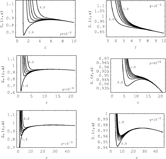
Figure 4: Specific energy of the equatorial circular orbits in Kerr–de Sitter black-hole spacetimes. The spacetimes are specified by the cosmological parameter $y$ and the rotational parameter $a$ ($a^{2}$ varies from 0.0 to 1.0 in steps of 0.2). The left column corresponds to the plus-family orbits; the right column corresponds to the minus-family orbits. The local extrema of the curves correspond to the marginally stable orbits, the rising parts correspond to stable orbits, and the descending parts correspond to unstable ones. The behavior of the curves for the spacetimes with $y<10^{-5}$ is similar to the case of $y=10^{-5}$.

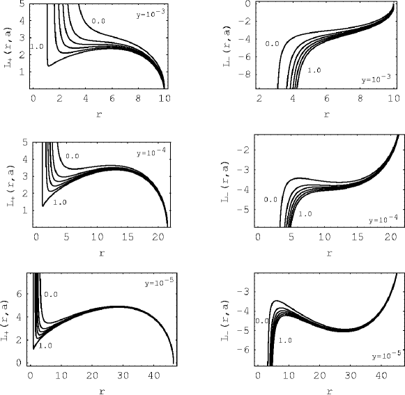
Figure 5: Specific angular momentum of the equatorial circular orbits in Kerr–de Sitter black-hole spacetimes. The spacetimes are specified by the cosmological parameter $y$ and the rotational parameter $a$ ($a^{2}$ varies from 0.0 to 1.0 in steps of 0.2). The left column corresponds to the plus-family orbits; the right column corresponds to the minus-family orbits. The local extrema of the curves correspond to the marginally stable orbits, the rising parts of $L_{+}$ and the descending parts of $L_{-}$ correspond to the stable orbits, the descending parts of $L_{+}$, and the rising parts of $L_{-}$ correspond to the unstable ones. The behavior of the curves for the spacetimes with $y<10^{-5}$ is similar to the case of $y=10^{-5}$.

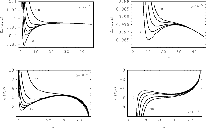
Figure 6: Specific energy and specific angular momentum of the equatorial circular orbits in Kerr–de Sitter naked-singularity spacetimes. The plus-family curves are plotted for the rotational parameter $a^{2}=10,20,30,50,100,300$; the minus-family curves are plotted for $a^{2}=2,5,10,20,30$. The meaning of particular parts of the curves is the same as in black-hole spacetimes.

In the limit of $y\rightarrow 0$, relations (38) and (LABEL:e40) reduce to the expression given by Chandrasekhar (in units of $M$) Chan:1983:BlackHoles: for circular orbits in the Kerr backgrounds:

$$E_{\pm}(r;a) = \frac{1-\frac{2}{r}\pm\frac{a}{r^{3/2}}}{\left[1-\frac{3}{r}\pm\frac{2a}{r^{3/2}}\right]^{1/2}},$$ (41)

$$L_{\pm}(r;a) = \pm r^{1/2}\frac{1+\frac{a^{2}}{r^{2}}\mp\frac{2a}{r^{3/2}}}{\left[1-\frac{3}{r}\pm\frac{2a}{r^{3/2}}\right]^{1/2}}.$$ (42)

In the limit of $a\rightarrow 0$ we arrive at the formulas determining the specific energy and the specific angular momentum of circular orbits in the field of Schwarzschild–de Sitter black holes Stu-Hle:1999:PHYSR4: :

$$E(r;y) = \frac{r-2-yr^{3}}{\left[r(r-3)\right]^{1/2}},$$ (43)

$$L(r;y) = \frac{r\left(1-yr^{3}\right)^{1/2}}{(r-3)^{1/2}};$$ (44)

here, we do not give $L$ for the minus-family orbits as these are equivalent to the plus-family orbits in spherically symmetric spacetimes.

The formulas for the specific energy and angular momentum of the equatorial circular orbits hold equally for both Kerr–de Sitter ($y>0$) and Kerr–anti-de Sitter ($y<0$) spacetimes. Here, we shall concentrate our discussion on the circular motion in Kerr–de Sitter spacetimes. We shall determine radii where the existence of circular orbits is allowed, the orientation of the circular motion relative to the locally nonrotating frames, stability of the circular motion relative to radial perturbations. Finally, we shall introduce the notion of marginally bound orbits.

IV.1 Existence of circular orbits

Inspecting expressions (38) and (LABEL:e40), we find two reality conditions on the circular orbits. The first restriction on the existence of circular orbits is given by the relation

$$y\leq y_{s}\equiv\frac{1}{r^{3}},$$ (45)

which introduces the notion of the “static radius,” given by the formula $r_{s}=y^{-1/3}$ independently of the rotational parameter $a$. It can be compared with the formally identical result in Schwarzschild–de Sitter spacetimes Stu-Hle:1999:PHYSR4: . A “free” or “geodetical” observer on the static radius has only $U^{t}$ component of four-velocity nonzero. The position on the static radius is unstable relative to radial perturbations, as follows from the discussion on stability of the circular orbits performed below.

The second restriction on the existence of circular orbits is given by the condition

$$1-\frac{3}{r}-a^{2}y\pm 2a\left(\frac{1}{r^{3}}-y\right)^{1/2}\geq 0;$$ (46)

the equality determines the radii of photon circular orbits, where both $E\rightarrow\infty$ and $L\rightarrow\pm\infty$.

The photon circular orbits of the plus-family are given by the relation

$$a=a^{(+)}_{ph(1,2)}(r;y)\equiv\frac{\left(1-yr^{3}\right)^{1/2}\pm\left(1-3yr^{2}\right)^{1/2}}{yr^{3/2}},$$ (47)

while for the minus-family orbits they are given by the relation

$$a=a^{(-)}_{ph(1,2)}(r;y)\equiv\frac{-\left(1-yr^{3}\right)^{1/2}\pm\left(1-3yr^{2}\right)^{1/2}}{yr^{3/2}}.$$ (48)

The photon circular orbits can be determined by a “common” formula related to $a^{2}$:

$$a^{2}=a^{2}_{ph(1,2)}(r;y)\equiv$$

$$\frac{\left(1-yr^{3}\right)+\left(1-3yr^{2}\right)\pm 2\sqrt{\left(1-yr^{3}\right)\left(1-3yr^{2}\right)}}{y^{2}r^{3}},$$

where the notation $a^{2}_{ph(1)}$ and $a^{2}_{ph(2)}$ is used for the $\pm$ parts of Eq. (LABEL:e53) because these functions can define photon orbits for both plus- (minus-) family circular orbits. A detailed discussion of the equatorial photon motion is presented in Stu-Hle:2000:CLAQG: , where more general, Kerr–Newman–(anti-)de Sitter spacetimes are studied. In the Kerr–de Sitter spacetimes the situation is much simpler. Since

$$\frac{\partial a^{2}_{ph(1,2)}}{\partial r}=\frac{\left[1-yr^{2}(r+3)+3y^{2}r^{5}\right]^{1/2}\left(yr^{2}-2\right)\pm\left[-2+yr^{2}(r+4)-y^{2}r^{5}\right]}{y^{2}r^{4}\left[1-yr^{2}(r+3)+3y^{2}r^{5}\right]^{1/2}},$$ (50)

we find that the local extrema of $a^{2}_{ph(1,2)}(r;y)$ are located at radii determined by the relation

$$y=y_{\mathop{\rm e}(ph)\pm}(r)\equiv\frac{2r+1\pm\sqrt{8r+1}}{2r^{3}}=y_{\mathop{\rm e}(h)\pm}(r).$$ (51)

Therefore, $a^{2}_{ph(1,2)}(r;y)$ and $a^{2}_{h}(r;y)$ have common points at their local extrema. Nevertheless, in order to obtain directly limits on the existence of the plus- (minus-) family circular orbits, it is convenient to consider the plus- (minus-) photon circular orbits determined by relations (47) and (48), respectively, under the assumption $a\geq 0$. We have to introduce a critical value of the rotational parameter corresponding to the situation where $a^{(+)}_{ph(1)}(r;y)=a^{(-)}_{ph(1)}(r;y)$—i.e., where these functions reach the static radius $r_{s}=y^{-1/3}$:

$$a^{2}_{c(s)}(y)\equiv\frac{1-3y^{1/3}}{y}.$$ (52)

Further, it is necessary to determine (by a numerical procedure) the related critical value of the cosmological parameter $y_{c(s)}$ such that for $y<y_{c(s)}$ the critical value $a^{2}_{c(s)}(y)$ corresponds to a naked-singularity spacetime. The numerical procedure implies

$$y_{c(s)}\doteq 0.033185.$$ (53)

The results can be summarized in dependence on the cosmological parameter and are illustrated in Fig. 7.

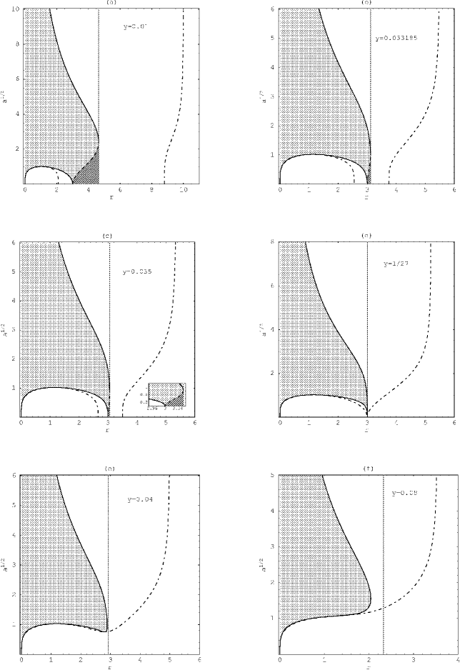
Figure 7: Existence of the circular orbits. Locations of the horizons and the photon circular orbits are given as functions of the rotational parameter for typical values of the cosmological parameter of Kerr–de Sitter spacetimes and the regions of the existence of the circular orbits are shown. Dash-dotted curves depict the horizons, solid curves depict the plus-family photon circular orbits, dashed curves depict the minus-family photon circular orbits, and the gray line gives the static radius ($r_{s}=y^{-1/3}$). Notice that the static radius is relevant only in the spacetimes admitting the minus-family circular orbits. The plus-family circular orbits exist in the whole shaded region, while the minus-family circular orbits exist in the dark-gray regions only—i.e., in the spacetimes with $y<y_{c(SdS)}$. In the naked-singularity spacetimes only one photon circular orbit exists and the plus-family orbits always approach the ring singularity at $r=0$.

1. $y\leq y_{c(s)}$ (Figs. 7a,7b)

   In black-hole spacetimes there are three photon circular orbits. Their loci satisfy the conditions

   $$r_{ph(1)}<r_{h(-)}<r_{h(+)}<r_{ph(2)}<r_{ph(3)}<r_{s}.$$ (54)

   The orbits $r_{ph(1)}$ and $r_{ph(2)}$ belong to the plus-family orbits, while $r_{ph(3)}$ belongs to the minus-family orbits. We can conclude that in the black-hole backgrounds, the plus-family circular orbits are located at radii satisfying the relations

   $$0<r<r_{ph(1)}\qquad\mbox{and}\qquad r_{ph(2)}<r<r_{s},$$ (55)

   while the minus-family orbits are located at radii satisfying the relation

   $$r_{ph(3)}<r<r_{s}.$$ (56)

   In the naked-singularity spacetimes, we have to distinguish two qualitatively different cases.

   If $a^{2}\leq a^{2}_{c(s)}(y)$, there is one photon circular orbit belonging to the minus-family orbits. In such spacetimes, the plus-family orbits are located in the region

   $$0<r<r_{s}.$$ (57)

   If $a^{2}>a^{2}_{c(s)}(y)$, the situation changes dramatically as the minus-family orbits (and the notion of the static radius) cease to exist. There is only one plus-family photon circular orbit. Therefore, the plus-family circular orbits are located in the region

   $$0<r<r_{ph}.$$ (58)

2. $y_{c(s)}<y\leq y_{c(SdS)}$ (Figs. 7c,7d)

   Now, we have to distinguish two cases in black-hole spacetimes.

   If $a^{2}\leq a^{2}_{c(s)}(y)$, the loci of the photon circular orbits are again related by relation (54), and the limits on the existence of plus-family and minus-family circular orbits are the same as in the case of $y<y_{c(s)}$—see relations (55) and (56), respectively.

   If $a^{2}>a^{2}_{c(s)}(y)$, black-hole spacetimes admit only the plus-family circular orbits and all of the three photon circular orbits limit them by the relation

   $$0<r<r_{ph(1)}\quad\mbox{and}\quad r_{ph(2)}<r<r_{ph(3)}.$$ (59)

   In naked-singularity spacetimes, only one plus-family photon circular orbit exists and the plus-family circular orbits are limited by relation (58).

3. $y_{c(SdS)}<y\leq y_{c(KdS)}$ (Fig. 7e)

   Only the plus-family circular orbits exist that are limited by three photon circular orbits through relation (59) in black-hole spacetimes and by one photon circular orbit through relation (58) in naked-singularity spacetimes.

4. $y_{c(KdS)}<y$ (Fig. 7f)

   Naked-singularity spacetimes exist for any $a>0$. The spacetimes admit only the plus-family circular orbits limited by one photon circular orbit through relation (58).

IV.2 Orientation of the circular orbits

The behavior of the circular orbits in the field of Kerr black holes ($y=0$) suggests that the plus-family orbits correspond to the corotating orbits, while the minus-family circular orbits correspond to the counterrotating ones. However, this statement is not generally correct even in some of the Kerr naked-singularity spacetimes—namely, in the spacetimes with the rotational parameter low enough, where counterrotating plus-family orbits could exist nearby the ring singularity Stu:1980:BULAI: . In Kerr–de Sitter spacetimes, the situation is even more complicated and we cannot identify the plus-family circular orbits with purely corotating orbits even in black-hole spacetimes. Moreover, in rotating spacetimes with a nonzero cosmological constant it is not possible to define the corotating (counterrotating) orbits in relation to stationary observers at infinity, as can be done in Kerr spacetimes, since these spacetimes are not asymptotically flat.

The natural way of defining the orientation of the circular orbits in Kerr–de Sitter spacetimes is to use the point of view of locally nonrotating frames that is used in asymptotically flat Kerr spacetimes too. The tetrad of one-forms corresponding to these frames in the Kerr–de Sitter backgrounds is given by Stu-Hle:2000:CLAQG:

$$\omega^{(t)}\equiv\left(\frac{\Delta_{r}\Delta_{\theta}\varrho^{2}}{I^{2}A}\right)^{1/2}{\rm d}t,$$ (60)

$$\omega^{(\varphi)}\equiv\left(\frac{A\sin^{2}\theta}{I^{2}\varrho^{2}}\right)^{1/2}({\rm d}\varphi-\Omega{\rm d}t),$$ (61)

$$\omega^{(r)}\equiv\left(\frac{\varrho^{2}}{\Delta_{r}}\right)^{1/2}{\rm d}r,$$ (62)

$$\omega^{(\theta)}\equiv\left(\frac{\varrho^{2}}{\Delta_{\theta}}\right)^{1/2}{\rm d}\theta,$$ (63)

where

$$A\equiv(r^{2}+a^{2})^{2}-a^{2}\Delta_{r},$$ (64)

$$\Delta_{\theta}\equiv 1+ya^{2}cos^{2}\theta,$$ (65)

and the angular velocity of the locally nonrotating frames,

$$\Omega\equiv\frac{{\rm d}\varphi}{{\rm d}t}=\frac{a}{A}\left[-\Delta_{r}+(r^{2}+a^{2})\Delta_{\theta}\right].$$ (66)

Note that $\Delta_{\theta}=1$ in the equatorial plane.

Locally measured components of the four-momentum are given by the projection of a particle’s four-momentum onto the tetrad:

$$p^{(\alpha)}=p^{\mu}\omega^{(\alpha)}_{\mu},$$ (67)

where

$$p^{\mu}=m\frac{{\rm d}x^{\mu}}{{\rm d}\tau}\equiv m\dot{x}^{\mu}=\frac{{\rm d}x^{\mu}}{{\rm d}\lambda}$$ (68)

are the coordinate components of particle’s four-momentum, the affine parameter $\lambda=\tau/m$, $m$ denotes the rest mass of the particle, and $\tau$ is its proper time.

In the equatorial plane, $\theta=\pi/2$, the azimuthal component of the four-momentum measured in the locally nonrotating frames is given by the relation

$$p^{(\varphi)}=\frac{mA^{1/2}}{Ir}\left(\dot{\varphi}-\Omega\dot{t}\right),$$ (69)

where the temporal and azimuthal components of the four-momentum, determined by the geodesic equations, can be expressed in the form containing the specific constants of motion $E,\ X$:

$$\dot{t} = \frac{I}{r^{2}}\left[aX+\frac{(r^{2}+a^{2})(r^{2}E-aX)}{\Delta_{r}}\right],$$ (70)

$$\dot{\varphi} = \frac{I}{r^{2}}\left[X+\frac{a}{\Delta_{r}}(r^{2}E-aX)\right].$$ (71)

A simple calculation reveals

$$p^{(\varphi)}=\frac{mr}{A^{1/2}}(aE+X)$$ (72)

and using Eq. (27) we obtain intuitively anticipated relation

$$p^{(\varphi)}=\frac{mr}{A^{1/2}}L.$$ (73)

We can see that the sign of the azimuthal component of the four-momentum measured in the locally nonrotating frames is given by the sign of the specific angular momentum of a particle on the orbit of interest. Therefore, the circular orbits with $p^{(\varphi)}>0$ $(L>0)$ we call corotating, and the circular orbits with $p^{(\varphi)}<0$ $(L<0)$ we call counterrotating, in agreement with the approach used in the case of asymptotically flat Kerr spacetimes.

IV.3 Stability of the circular orbits

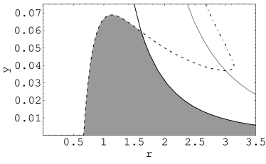
Figure 8: Reality conditions for the existence of the stable circular orbits. Black and gray solid curves correspond to the functions $y_{ms}(r)$ and $y_{s}(r)$, respectively; dash-dotted and dashed curves correspond to the functions $y_{ms+}(r)$ and $y_{ms-}(r)$, respectively. Stable orbits can exist only in the shaded region, where the local maximum corresponds to the critical value of the cosmological parameter $y_{\rm crit(ms+)}\doteq 0.06886$.

The loci of the stable circular orbits are given by the condition

$$\frac{\mbox{d}^{2}R}{\mbox{d}r^{2}}\geq 0,$$ (74)

which has to be satisfied simultaneously with the conditions $R(r)=0$ and $\mbox{d}R/\mbox{d}r=0$ determining the specific energy and the specific angular momentum of the circular orbits. Using relations (38) and (39), we find that the radii of the stable orbits of both families are restricted by the condition

$$r\left[6-r+r^{3}(4r-15)y\right]\mp$$

$$\mp 8a\left[r\left(1-yr^{3}\right)^{3}\right]^{1/2}+a^{2}\left[3+r^{2}y\left(1-4yr^{3}\right)\right]\geq 0.$$

The marginally stable orbits of both families can be described together by the relation

$$a^{2}=a^{2}_{ms(1,2)}(r;y) \equiv \left[3+r^{2}y\left(1-4yr^{3}\right)\right]^{-2}r\left\{\left[r-6-r^{3}(4r-15)y\right]\right.$$ (76)

$$\times\left[3+r^{2}y\left(1-4yr^{3}\right)\right]+32\left(1-yr^{3}\right)^{3}\pm 8\left(1-yr^{3}\right)^{3/2}\left(1-4yr^{3}\right)^{1/2}$$

$$\times\left.\left\{r\left[3-ry\left(6+10r-15yr^{3}\right)\right]-2\right\}^{1/2}\right\}.$$

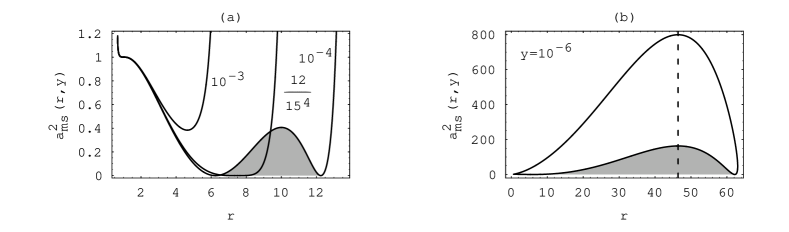
Figure 9: Marginally stable circular orbits in Kerr–de Sitter spacetimes. The relevant functions are given for some typical values of the cosmological parameter $y$. (a) The black-hole region of Kerr–de Sitter spacetimes. For $y<12/15^{4}$ there exist spacetimes containing four marginally stable (ms) orbits. For a given spacetime, the innermost and the outermost ms orbits belong to the plus-family orbits; the two orbits in between belong to the minus-family orbits. (b) In the naked-singularity region there exist spacetimes with no stable orbits for a fixed value of $y$ [spacetimes with $a^{2}$ greater than the global maximum of function $a^{2}_{ms}(r;y)$ for a given $y$]. Stable counterrotating (minus-family) orbits exist only in shaded regions of the presented spacetimes. But some naked-singularity spacetimes contain counterrotating plus-family orbits; for more details, see the text. The dashed line corresponds to the radius $(10y)^{-1/3}$ where both maxima of $a^{2}_{ms}(r;y)$ are located.

The ($\pm$) sign in Eq. (76) is not directly related to the plus-family and minus-family orbits. The function $a^{2}_{ms(1)}$, corresponding to the $+$ sign in Eq. (76), determines marginally stable orbits of the plus-family orbits, while the function $a^{2}_{ms(2)}$, corresponding to the $-$ sign in Eq. (76), is relevant for both the plus-family and minus-family orbits. The reality conditions for the functions $a^{2}_{ms(1,2)}(r;y)$ are directly given by Eq. (76). The standard condition $y\leq y_{s}(r)\equiv 1/r^{3}$ is guaranteed by the first relevant condition

$$y\leq y_{ms}(r)\equiv\frac{1}{4r^{3}}.$$ (77)

The other two conditions can be given in the form

$$y\leq y_{ms-}(r)\qquad\mbox{or}\qquad y\geq y_{ms+}(r),$$ (78)

where the functions $y_{ms(\pm)}(r)$ are given by the relation

$$y_{ms\pm}(r)=\frac{3+5r\pm\left(60r-20r^{2}+9\right)^{1/2}}{15r^{3}}.$$ (79)

The behavior of the functions $y_{s}(r)$, $y_{ms}(r)$, and $y_{ms{\pm}}(r)$ is illustrated in Fig. 8. The function $y_{ms(+)}(r)$ is irrelevant; the relevant function $y_{ms(-)}(r)$ intersects the function $y_{s}(r)$ at $r=3$, where $y=y_{c(SdS)}=1/27$, and the function $y_{ms}(r)$ at $r=(3+2\sqrt{3})/4$, where $y=y_{i}=16/(3+2\sqrt{3})^{3}$. The critical value of the cosmological parameter for the existence of the stable (plus-family) orbits, corresponding to the local maximum of $y_{ms(-)}(r)$, is given by

$$y_{crit(ms+)}=\frac{100}{(5+2\sqrt{10})^{3}}\doteq 0.06886.$$ (80)

The related critical value of the rotational parameter is

$$a^{2}_{crit(ms+)}=\frac{955+424\sqrt{10}}{1620}\doteq 1.41716.$$ (81)

The plus-family stable circular orbits are allowed for $y<y_{ms}(r)$, if $y<y_{i}$, and for $y<y_{ms(-)}(r)$, if $y_{i}<y<y_{crit(ms+)}$.

The condition determining the local extrema of $a^{2}_{ms(1,2)}(r;y)$,

$$\frac{\partial a^{2}_{ms(1,2)}(r;y)}{\partial r}=0,$$ (82)

implies very complicated relations; however, they lead to one simple relevant relation

$$y=y_{\mathop{\rm e}(ms)}(r)\equiv\frac{1}{10r^{3}}$$ (83)

determining important local extrema of both $a^{2}_{ms(1,2)}(r;y)$ simultaneously, both located on the radius

$$r=r_{e(ms)}(y)\equiv\frac{1}{(10y)^{1/3}}.$$ (84)

The critical value of the cosmological parameter for the existence of the minus-family stable circular orbits, determined by the condition $a^{2}_{ms(2)}(r_{e(ms)};y)=0$, is given by

$$y_{crit(ms-)}=\frac{12}{15^{4}}.$$ (85)

It coincides with the limit on the existence of the stable circular orbits in Schwarzschild–de Sitter spacetimes Stu-Hle:1999:PHYSR4: .

Properties of the functions $a^{2}_{ms(1,2)}(r;y)$ can be summarized in the following way.

1. $y>y_{crit(ms+)}$. No stable circular orbits are allowed for any value of the rotational parameter.

2. $y_{crit(ms+)}>y>y_{crit(ms-)}$. At $r=r_{e(ms)}$, the function $a^{2}_{ms(1)}(r;y)$ has a local maximum ($a^{2}_{ms(max)}$), and the function $a^{2}_{ms(2)}(r;y)$ has a local minimum ($a^{2}_{ms(min)}$). For $a^{2}_{ms(min)}<a^{2}<a^{2}_{ms(max)}$, the equation $a^{2}=a^{2}_{ms(1,2)}(r;y)$ determines two marginally stable plus-family circular orbits (an inner one and an outer one). For $0<a^{2}<a^{2}_{ms(min)}$ and $a^{2}>a^{2}_{ms(max)}$, no stable circular orbits are allowed.

3. $y<y_{crit(ms-)}$. There are two zero points of the function $a^{2}_{ms(2)}(r;y)$ corresponding to its local minima, while it has a local maximum $a^{2}_{ms(max2)}$ at $r=r_{e(ms)}$, where the maximum of the function $a^{2}_{ms(1)}(r;y)$ is located too. For $a^{2}>a^{2}_{ms(max)}$, there is no stable circular orbit. For $a^{2}_{ms(max2)}<a^{2}<a^{2}_{ms(max)}$, there are two marginally stable plus-family circular orbits. For $a^{2}<a^{2}_{ms(max2)}$, there are four marginally stable orbits. The innermost and the outermost orbits belong to the plus-family orbits; the two orbits in between belong to the minus-family orbits.

The functions $a^{2}_{ms(1,2)}$ are illustrated for typical values of the cosmological parameter in Fig. 9. In the parameter space $y$-$a^{2}$, separation of Kerr–de Sitter spacetimes according to the existence of stable circular orbits, determined by the functions $a^{2}_{ms(1,2)}(r;y)$ and $y_{e(ms)}(r)$, is given in Fig. 3.

IV.4 Marginally bound circular orbits

Figure 10: Effective potential of the equatorial radial motion of test particles in an appropriatelly chosen Kerr–de Sitter black-hole spacetime ($y=10^{-4},\ a^{2}=0.36$) allowing stable circular orbits for corotating particles. Marginally bound (mb) orbits are given by the solid curve corresponding to the angular momentum parameter $X=X_{mb+}\doteq 2.38445$. The curve has two local maxima of the same value, $E_{mb}\doteq 0.93856$, corresponding to the inner [mb(i)] and the outer [mb(o)] marginally bound orbits. The dashed effective potential defines the inner marginally stable orbit [ms(i)] by coalescing the local minimum and the (inner) local maximum. It corresponds to the parameter $X=X_{ms(i)+}\doteq 2.20307$ with specific energy $E_{ms(i)+}\doteq 0.90654$. In an analogous manner, the dash-dotted potential defines the outer marginally stable orbit [ms(o)] with specific energy $E_{ms(o)+}\doteq 0.94451$ corresponding to the parameter $X=X_{ms(o)+}\doteq 2.90538$.

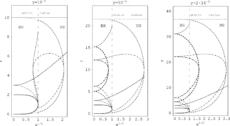
Figure 11: Mutual positions of the astrophysically important circular orbits in Kerr–de Sitter spacetimes. The figures are constructed for three representative values of $y$. The radii of the special equatorial circular orbits are plotted as functions of the rotational parameter $a$. The wide dashed line is given by the value of rotational parameter corresponding to the extreme black hole and it splits up Kerr–de Sitter spacetimes into black-hole (BH) and naked-singularity (NS) regions. Thin curves are used for the plus-family orbits (in the most cases they correspond to the corotating orbits from the point of view of the locally nonrotating observers, but there are exceptions described in the text). Bold curves are used for the minus-family orbits (in all spacetimes under consideration: counterrotating orbits). Solid curves determine the inner and outer black-hole horizons. Dotted curves determine the photon circular orbits; dashed curves determine the marginally bound (mb) circular orbits. There is a disconnection between BH and NS regions for the plus-family orbits. Lower gray dashed curves determine the marginally bound orbits hidden under the inner black-hole horizon; the upper one, approaching the static radius for small $a$, is its outer analogy. Dash-dotted curves determine the marginally stable (ms) orbits. For $y\geq 12/15^{4}$ there are no minus-family mb and ms orbits.

The behavior of the effective potential (28) enables us to introduce the notion of the marginally bound orbits—i.e., unstable circular orbits where a small radial perturbation causes infall of a particle from the orbit to the center or its escape to the cosmological horizon. For some special value of the axial parameter $X$, denoted as $X_{mb}$, the effective potential has two local maxima related by the condition

$$E_{(+)}(r_{mb(i)};X_{mb},a,y)=E_{(+)}(r_{mb(o)};X_{mb},a,y),$$ (86)

and corresponding to both the inner and outer marginally bound orbits; see Fig. 10 (and Fig. 15, below). For completeness, the figures include the effective potentials defining both the inner and outer marginally stable orbits (corresponding to special values of the parameter $X$: $X_{ms(i)},\ X_{ms(o)}$). The search for the marginally bound orbits in a concrete Kerr–de Sitter spacetime must be realized in a numerical way and can be successful only in the spacetimes admitting stable circular orbits. Clearly, in the spacetimes with $y\geq 12/15^{4}$, the minus-family marginally bound orbits do not exist. Figure 3 offers insight into the possibility of the existence of both stable and bound circular orbits of both families. The limiting (solid) curves are obtained from the conditions (76), (83) that have to be solved simultaneously.

The location of the astrophysically important circular orbits (photon orbits, marginally stable and marginally bound orbits) in dependence on the rotational parameter $a$ is given in Fig. 11 for three appropriately chosen values of the cosmological parameter $y$. The values of $y$ reflect the dependence of the existence of stable minus-family orbits on $y$. Stable plus-family orbits exist for all chosen values of $y$ in the relevant range of the parameter $a$. Spacetimes without stable circular orbits or without any circular orbits are inferred from Figs. 7, 8.

V Discussion

Figure 12: Circular orbits with zero angular momentum. The function $y_{(L=0)}(r;a)$ is plotted for $a^{2}=\{1,1.8,2.4406,5\}$. For $a^{2}=1$, when the black-hole spacetimes are allowed, the first two orbits are hidden under the black-hole event horizon. The dashed curve determines horizons of Kerr–de Sitter spacetimes with $a^{2}=1$. In the other cases only naked-singularity spacetimes are allowed and even three $L=0$ orbits are possible for $a^{2}<2.4406$. The case $a^{2}\doteq 2.4406$ (the curve with an inflex point at $y\doteq 0.03998$) corresponds to the maximum value of the rotational parameter addmiting the stable counterrotating plus-family orbits.

In comparison with asymptotically flat Kerr spacetimes, where the effect of the rotational parameter vanishes for asymptotically large values of the radius, in Kerr–de Sitter spacetimes the properties of the circular orbits must be treated more carefully, because the rotational effect is relevant in whole the region where the circular orbits are allowed and it survives even at the cosmological horizon.

The minus-family orbits have specific angular momentum negative, $L_{-}<0$, in every Kerr–de Sitter spacetime and such orbits are counterrotating from the point of view of locally nonrotating frames.

In black-hole spacetimes, the plus-family orbits are corotating in almost all radii where the circular orbits are allowed except some region in vicinity of the static radius, where they become counterrotating, as their specific angular momentum $L$ is slightly negative there. In naked-singularity spacetimes, the plus-family orbits behave in a more complex way; nevertheless, they are always counterrotating in vicinity of the static radius.

The specific angular momentum of particles located on the static radius, where the plus-family orbits and the minus-family orbits coalesce, is given by the relation

$$L(r_{s};y,a)=L_{s}\equiv-a\frac{3y^{1/3}+a^{2}y}{\left(1-3y^{1/3}-a^{2}y\right)^{1/2}},$$ (87)

and their specific energy is

$$E(r_{s};y,a)=E_{s}\equiv(1-3y^{1/3}-a^{2}y)^{1/2}.$$ (88)

V.1 Circular orbits with zero angular momentum

Separation of the corotating and counterrotating orbits as defined by their azimuthal angular momentum relative to the locally nonrotating frames is determined by the orbits with $L=0$. The orbits with zero angular momentum are defined by the relation

$$y=y_{(L=0)}(r;a)\equiv\frac{-r[r(r^{2}+a^{2})+4a^{2}]+r^{1/2}(r^{2}+a^{2})^{1/2}\left[(r^{2}+a^{2})(r^{3}+4a^{2})+8a^{2}r^{2}\right]^{1/2}}{2a^{2}r^{2}(r^{2}+a^{2})}.$$ (89)

At these orbits, the locally nonrotating observers follow circular geodesics at the equatorial plane.

The physically relevant zero points of the function $y_{(L=0)}$ are given by the function

$$a_{z(L=0)}(r)\equiv r^{1/2}[1+(1-r)^{1/2}]$$ (90)

determining circular orbits with $L=0$ in the asymptotically flat Kerr backgrounds. A detailed study reveals that such orbits exist only in Kerr naked-singularity spacetimes with $1<a/M\leq\frac{3}{4}\sqrt{3}$. (In Kerr black-hole spacetimes orbits of this kind are hidden under the event horizon.) The typical behavior of the function $y_{(L=0)}(r;a)$ is presented in Fig. 12 for some appropriately chosen values of the rotational parameter $a^{2}$. The function has a local extremum for $a^{2}<a^{2}_{cL}\equiv 2.4406$ (where the critical value $a^{2}_{cL}$ is obtained by a numerical procedure)—we can conclude that up to three zero-angular-momentum orbits can exist in the corresponding Kerr–de Sitter spacetimes. In the naked-singularity spacetimes all three orbits with zero angular momentum are relevant and the middle orbit is stable. In black-hole spacetimes, however, two of these orbits are hidden under the black-hole horizons and only the unstable one, located nearby the static radius, is physically important. The plus-family orbits between the zero-angular-momentum orbit and the static radius are counterrotating. Comparison of the functions $y_{(L=0)}(r;a)$ and $y_{ms}(r;a)$ (determining the position of the outermost marginally stable orbit for a given cosmological parameter $y$) reveals that the discussed orbits are unstable.

In naked-singularity spacetimes, the behavior of the plus-family orbits is more intriguing. Except for the unstable counterrotating orbits located nearby the static radius (discussed above), some stable counterrotating plus-family circular orbits exist in the vicinity of the ring singularity of naked-singularity spacetimes with rotational parameter low enough. Spacetimes admitting such orbits belong to the dash-dotted naked-singularity region of the parametric space $(y,a^{2})$ presented in Fig. 3. The limiting (dash-dotted) curve was obtained by solving simultaneously the conditions for the marginally stable orbits given by Eq. (76) and the condition for the orbits with zero angular momentum given by Eq. (89).

In a given Kerr–de Sitter naked-singularity spacetime relations (76), (89) determine the innermost and outermost stable counterrotating plus-family orbits, respectively.

V.2 Circular orbits with negative energy

In the rotating naked-singularity spacetimes the potential well can be deep enough nearby the ring singularity to allow the existence of stable (plus-family) counterrotating circular orbits with negative specific energy, indicating an extremely high efficiency of conversion of the rest mass into heat energy during accretion in a corotating (or, more precisely, a plus-family) thin disk. The plus-family circular orbits with zero energy are given by the relation

$$y=y_{(E=0)}(r;a)\equiv\frac{r[2(r^{2}+a^{2})(r-2)-a^{2}r]+ar^{1/2}\{4(r^{2}+a^{2})^{2}-r^{2}[4(r^{2}+a^{2})(r-2)-a^{2}r]\}^{1/2}}{2r^{2}(r^{2}+a^{2})^{2}}.$$ (91)

The reality conditions of the function $y_{(E=0)}(r;a)$ are given by the relations

$$r\geq 0,$$ (92)

$$4(r^{2}+a^{2})^{2}-r^{2}[4(r^{2}+a^{2})(r-2)-a^{2}r]\geq 0.$$ (93)

The condition (93) can be transferred into the relation

$$a^{2}\geq a^{2}_{min(E=0)}(r)\equiv\frac{r^{2}}{8}[3r-16+(9r^{2}-32r+64)^{1/2}],$$ (94)

which is relevant for $r>3$. For $0<r<3$ the function $a^{2}_{min(E=0)}(r)$ is negative. The zero points of the function $y_{(E=0)}(r;a)$ are given by the function

$$a_{z(E=0)}(r)\equiv r^{1/2}(2-r),$$ (95)

which determines the circular orbits with zero specific energy in Kerr spacetimes. For $y=0$, such orbits exist only in Kerr naked-singularity spacetimes with $1<a/M\leq\frac{4}{3}\sqrt{\frac{2}{3}}$, which are a subset of spacetimes with zero-angular-momentum orbits; in fact, orbits with $E=0$ have $L<0$ (for details see Stu:1980:BULAI: ). The behavior of the function $y_{(E=0)}(r;a)$ is presented for some typical values of the rotational parameter $a$ in Fig. 13.

Figure 13: Location of the plus-family orbits with $E=0$. The dashed curves determine the horizons of Kerr–de Sitter spacetimes. The solid curves determine the orbits with $E=0$. The rising (descending) part of $y_{(E=0)}(r;a)$ corresponds to the stable (unstable) orbits. The intervals of the rotational parameter giving different behavior of the curves $y_{(E=0)}(r;a)$, $y_{h}(r;a)$ in cases (a)–(g) are (a) $0<a^{2}<1$, (b) $1<a^{2}<1.06992$, (c) $1.06992<a^{2}<a^{2}_{c(E=0)}\doteq 1.18518$, (d) $a^{2}_{c(E=0)}<a^{2}<a^{2}_{\rm{crit}}\doteq 1.21202$, (e) $a^{2}_{\rm{crit}}<a^{2}<1.25976$, (f) $1.25976<a^{2}<a^{2}_{s(E=0)}\doteq 1.47000$, (g) $a^{2}>a^{2}_{s(E=0)}$.

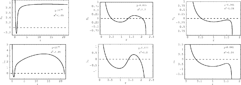
Figure 14: Naked-singularity spacetimes admitting stable circular orbits with negative specific energy. We can see that stable circular orbits in vicinity of the innermost stable orbit (the left and middle columns) or even all the stable orbits (the right column) can have negative energy. The behavior of the specific angular momentum reveals counterrotation of such orbits.

In Kerr–de Sitter spacetimes with $0<a^{2}<1.47$, the function $y_{(E=0)}$ has two local extrema leading up to three circular orbits with zero energy. The ending points of the curves are given by the condition (94) and are represented by the function

$$y_{min(E=0)}(r)\equiv y_{(E=0)}(r;a=a_{min(E=0)})=$$

$$\frac{3r^{2}-10r+16-(r-2)(9r^{2}-32r+64)^{1/2}}{2r^{4}}.$$

Details of the properties of the plus-family orbits with $E=0$ can be inferred from Fig. 13. Here, we give a short overview of them.

In the black-hole spacetimes, there is always one orbit with $E=0$ located under the inner black-hole horizon, and there can exist, for properly chosen parameters $a$ and $y$, one orbit with $E=0$ located above the outer black-hole horizon. Both the orbits must be unstable relative to radial perturbations.

In the naked-singularity spacetimes, if $a^{2}<a^{2}_{c(E=0)}\doteq 1.18518$, there can exist one orbit with $E=0$ (unstable), two such orbits (the inner one unstable, the outer one stable), or three such orbits (the inner and outer being unstable, the intermediate being stable). If $a^{2}>a^{2}_{c(E=0)}$ and $y$ is properly chosen, there can be an additional possibility of the nonexistence of the circular orbit with $E=0$. If $a^{2}>a^{2}_{s(E=0)}\doteq 1.47000$, there can exist no stable zero-energy orbits for any $y$ (cf. Fig. 3).

Examples of naked-singularity spacetimes admitting stable counterrotating plus-family circular orbits with negative energy are presented in Fig. 14. The efficiency of conversion of the rest mass into heat energy during accretion, given by the relation

$$\eta\equiv E_{ms(o)}-E_{ms(i)},$$ (97)

is limited by the specific energy of the outermost stable circular plus-family orbit, $E_{ms(o)}<1$, which can be directly inferred from Fig. 15.

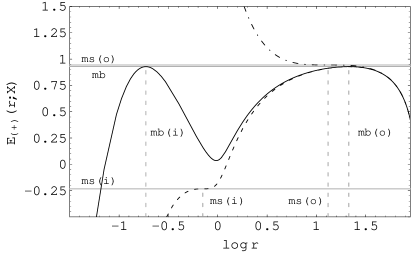
Figure 15: Effective potential of the equatorial radial motion of test particles in an appropriately chosen Kerr–de Sitter naked-singularity spacetime ($y=10^{-4},\ a^{2}=1.05$) allowing the stable circular orbits with negative energy. Marginally bound (mb) orbits are given by the solid curve corresponding to $X=X_{mb+}\doteq-0.18444$. The curve has two local maxima of the same value, $E_{mb}\doteq 0.92857$, corresponding to the inner [mb(i)] and the outer [mb(o)] marginally bound orbits. The dashed effective potential defines the inner marginally stable orbit [ms(i)] resulting from coalescence of the local minimum and (inner) local maximum, with $X=X_{ms(i)+}\doteq-0.40713$ and the specific energy $E_{ms(i)+}\doteq-0.23321$. In an analogous manner, the dash-dotted potential defines the outer marginally stable orbit [ms(o)] with the specific energy $E_{ms(o)+}\doteq 0.94405$ and $X=X_{ms(o)+}\doteq 2.40379$.

Correspondingly, extraction of the rotational energy from a naked singularity with rotational parameter low enough is possible with subsequent conversion of the naked singularity into a black hole (see, e.g., Stu:1981:BULAI: ). Spacetimes allowing such processes are contained in the shaded naked-singularity region of the parametric space $(y,a^{2})$ in the Fig. 3. The limiting (dotted) curve was obtained by solving simultaneously conditions for the marginally stable orbits (76) and the circular orbits with $E=0$ (91).

VI Concluding remarks

Figure 16: Specific energy of the marginally stable minus-family orbits [(a) Inner, (b) Outer] and (c) the accretion efficiency $\eta_{-}\equiv E_{ms(o)-}-E_{ms(i)-}$ given as a function of the rotational parameter for three representative values of the cosmological parameter. For Kerr spacetimes, $y=0$, we assume $E_{ms(o)-}=1$.

Many properties of Kerr–de Sitter spacetimes and circular orbits of both families can be clearly viewed from figures which are presented in the paper. Table 1 contains a certain classification of the figures which could be helpful for quick orientation in the topic.

Table 1: Classification of the figures.

Spacetime properties	Figs. 1–3
Properties	$(+)$ family	$(-)$ family
of circular orbits
General	Figs. 7–11, 15	Figs. 7–9, 11
Specific energy	Figs. 4, 6, 13, 14, 17–19	Figs. 4, 6, 16
Spec. ang. mom.	Figs. 5, 6, 12, 19	Figs. 5, 6, 12
Accretion efficiency	Figs. 17, 18	Fig. 16

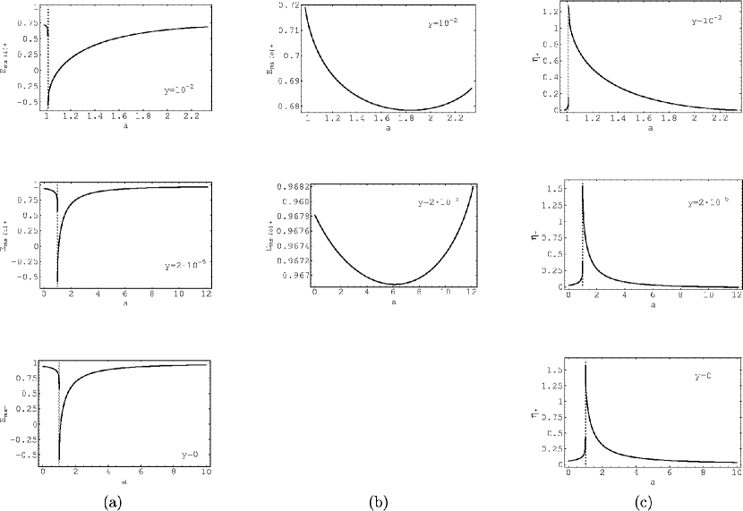
Figure 17: Specific energy of the marginally stable plus-family orbits [(a) Inner, (b) Outer] and (c) the accretion efficiency $\eta_{+}\equiv E_{ms(o)+}-E_{ms(i)+}$ (right column) as a function of the rotational parameter for three representative values of the cosmological parameter. The gray line corresponds to the extreme black hole. We can see a strong discontinuity of the specific energy of the inner marginally stable orbits and the accretion efficiency when black holes and naked singularities approach the extreme black-hole state. For Kerr spacetimes, $y=0$, we assume $E_{ms(o)+}=1$.

Both black-hole and naked-singularity Kerr–de Sitter spacetimes can be separated into three classes according to the existence of stable (and, equivalently, marginally bound) circular orbits (see Fig. 3). Stable orbits of both the plus family and minus family exist in the spacetimes of class I (black holes) and class V (naked singularities). Solely stable orbits of the plus family exist in the spacetimes of classes II (black holes) and VI (naked singularities). No stable orbits exist in the spacetimes of classes III and IV. In dependence on the cosmological parameter, there are three qualitatively different types of the behavior of the loci of the marginally stable, marginally bound, and photon circular orbits as functions of the rotational parameter. These functions are illustrated for three representative values of $y$ in Fig. 11, enabling us to make in a straightforward way separation of Kerr–de Sitter spacetimes into classes I–VI. In the special case of Kerr spacetimes ($y=0$), these functions can be found in Bar:1973:BlaHol: ; Stu:1980:BULAI: .

The marginally stable circular orbits are crucial in the context of Keplerian (geometrically thin) accretion disks as these orbits determine the efficiency of conversion of rest mass into heat energy of any element of matter transversing the disks from their outer edge located on the outer marginally stable orbit to their inner edge located on the inner marginally stable orbit.

Clearly, accretion disks constituted from minus-family orbits are everywhere counterrotating relative to the locally nonrotating frames. For the minus-family disks, the specific energy of both the outer and inner marginally stable circular orbits and the efficiency parameter $\eta_{-}=E_{ms(o)-}-E_{ms(i)-}$ are given for three typical values of $y$ as functions of $a$ in Fig. 16. In the limit of $a\rightarrow 0$ with $y$ being fixed, we obtain the known values of the specific energy $E_{ms(o)}$, $E_{ms(i)}$ and the efficiency parameter of the accretion process $\eta$ for the Schwarzschild–de Sitter black holes Stu-Hle:1999:PHYSR4: . Both the specific energy parameters $E_{ms(o)-}(a)$, $E_{ms(i)-}(a)$ and the efficiency $\eta_{-}(a)$ vary smoothly at values of the rotational parameter corresponding to the extreme black holes.

The Keplerian accretion disks constituted from the plus-family orbits behave in much more complex way in comparison with those of the minus-family orbits. First, usually these disks could be considered as corotating relative to the locally nonrotating frames; recall that in asymptotically flat Kerr black-hole spacetimes the plus-family disks are corotating at all radii down to the marginally stable orbit, while in the field of naked singularities with $a/M<\frac{3}{4}\sqrt{3}$ the stable circular orbits corotating at large distances are transformed into counterrotating orbits in vicinity of the marginally stable orbit Stu:1980:BULAI: . A similar behavior occurs in Kerr–de Sitter spacetimes; however, in the spacetimes with $y\rightarrow y_{c(KdS)}$, the stable plus-family orbits can be counterrotating even at all allowed radii (see, e.g., Fig. 14). (Moreover, there are always counterrotating plus-family orbits in the vicinity of the static radius, where the plus-family orbits and the minus-family orbits coalesce; these orbits are, however, unstable relative to radial perturbations and cannot be related to accretion disks.)

Figure 18: Specific energy of the marginally stable orbits and accretion efficiency near the extreme black-hole states. (a) Specific energy of the inner marginally stable plus-family orbit in extreme black-hole and related limiting naked-singularity spacetimes approaching the extreme hole states as a function of the cosmological parameter $y$. The solid curve corresponds to the extreme black holes; the dashed curve corresponds to the limiting naked singularities. The curves are symmetric around the zero-energy axis and tend to zero for $y=y_{c(KdS)}$. In extreme Kerr spacetimes ($y=0$), the specific energies in the black-hole and naked-singularity cases are $1/\sqrt{3}$ and $-1/\sqrt{3}$, respectively. (b) Specific energy of the outer marginally stable plus-family orbit in extreme Kerr–de Sitter black-hole spacetimes is the same as for naked-singularity spacetimes approaching the extreme hole state; i.e., there is no discontinuity in this case. The specific energy tends to zero for $y\to y_{c(KdS)}$. (c) Accretion efficiency for the extreme black holes $\eta_{bh}$ (solid curve) and for the limiting naked singularities $\eta_{ns}$ (dashed curve). For $y=0$ (pure Kerr spacetimes) we obtain the maximum value $0.42$ for black holes and $1.58$ for naked singularities. For $y\to y_{c(KdS)}$ the efficiency tends to zero for both black holes and naked singularities.

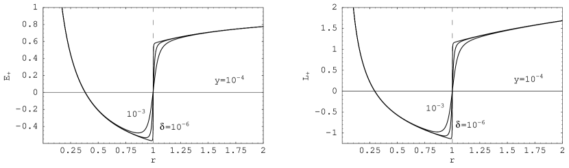
Figure 19: Distribution of the specific energy and the specific angular momentum of the equatorial circular orbits in naked-singularity spacetimes approaching the extreme black-hole state. The orbits with the specific energy in the interval $E_{ms(ns)}<E<E_{ms(bh)}$ are located in an extremely small interval of the radial coordinate having, however, an extremely long proper length Bar:1973:BlaHol: . After conversion of a hypothetical naked singularity into an extreme black hole all these circular orbits become unstable relative to radial perturbations and will be immediately swallowed by the black hole. The figures are drawn for $a=a_{0}(1+\delta)$ and $y=y_{0}(1-\delta)$, where $y_{0}=10^{-4}$ and $a_{0}=1.0001$ are chosen to correspond to an extreme black hole and, subsequently, $\delta=10^{-3},10^{-4},10^{-6}$.

Second, the specific energy $E_{ms(i)+}(y,a)$ of the inner marginally stable plus-family orbit can be negative. Recall that $E_{ms(i)+}<0$ in asymptotically flat Kerr naked-singularity spacetimes with the rotational parameter $a/M<\frac{4}{3}\sqrt{\frac{2}{3}}$, indicating the efficiency of the accretion process $\eta_{+}=E_{ms(o)+}-E_{ms(i)+}>1$, because in asymptotically flat Kerr spacetimes the outer edge of the accretion disks can be at arbitrarily large radii, implying thus $E_{ms(o)+}=1$. In Kerr–de Sitter spacetimes allowing $E_{ms(i)+}<0$, the efficiency of the accretion process can be both $\eta>1$ and $\eta<1$, as it depends strongly on $E_{ms(o)+}$, which for $y\sim y_{c(KdS)}$ can be even negative (see Fig. 14). For three typical values of $y$, the functions $E_{ms(o)+}(a)$, $E_{ms(i)+}(a)$, $\eta_{+}(a)$ are illustrated in Fig. 17. The specific energy function $E_{ms(i)+}(a)$ falls for $a$ growing in the black-hole region and for $a$ descending in the naked-singularity region. The specific energy function $E_{ms(o)+}(a)$ has a local minimum at some value of the rotational parameter $a$ strongly dependent on the cosmological parameter $y$. For $y$ being fixed, the accretion efficiency $\eta_{+}(a)$ grows for $a$ growing in the black-hole sector up to the critical value corresponding to the extreme black-hole spacetime, and it also grows for $a$ descending in the naked-singularity sector down to the critical value.

Third, there is a strong discontinuity of the specific energy function $E_{ms(i)+}(a)$ for spacetimes approaching the extreme black hole state from the black-hole and the naked-singularity sectors. For extreme Kerr black holes ($y=0,a/M=1$), there is the limiting value of the specific energy $E_{ms(bh)}=1/\sqrt{3}$, while for naked singularities approaching the extreme hole states ($a/M\rightarrow 1$ from above), there is $E_{ms(ns)}=-1/\sqrt{3}$. For extreme Kerr–de Sitter spacetimes, the dependence of the specific energy of the inner marginally stable orbit on the cosmological parameter is shown in Fig. 18a. Clearly, there is $E_{ms(ns)}(y)=-E_{ms(bh)}(y)$, where for a given cosmological parameter $y$ the rotational parameter $a$ of the corresponding extreme black hole is determined by the upper branch of the limiting line separating black-hole and naked-singularity states in Fig. 3. For $y\rightarrow y_{c(KdS)}$, there is $E_{ms(bh)}(y)\rightarrow 0$. For the specific energy function $E_{ms(o)+}(y,a)$ of the outer marginally stable orbits there is no discontinuity at the states corresponding to extreme black-hole spacetimes (see Fig. 18b). The accretion efficiency $\eta_{+}(y)$ in the field of extreme black holes [$\eta_{bh}(y)$] and in the field of the naked singularities infinitesimally close to the extreme hole states [$\eta_{ns}(y)$] is shown in Fig. 18c. For $y=0$ their difference takes the maximum ($\eta_{ns}=1+1/\sqrt{3}$, $\eta_{bh}=1-1/\sqrt{3}$), while at $y=y_{c(KdS)}$ the difference vanishes ($\eta_{ns}=0$, $\eta_{bh}=0$).

As a result of accretion in a plus-family or a minus-family Keplerian disk, a hypothetical naked singularity can be converted into an extreme black hole. In the case of Kerr naked singularities their evolution into an extreme hole state was discussed in Cal-Nob:1979:NUOC2: ; Stu:1981:BULAI: ; Stu-Pls-Hle:2002:PERSEUS:EvoKerrNakSin . Such a conversion can be a rather dramatic process in the case of the plus-family accretion disks, because of the discontinuity of the plus-family orbits at the extreme black-hole state. We can understand this process if we show how the stable circular orbits are distributed in naked-singularity spacetimes approaching the extreme black-hole state (Fig. 19). We can see that all the orbits with the specific energy ranging from $E_{ms(ns)}(y)$ up to $E_{ms(bh)}(y)$ are distributed at an infinitesimally small range of the radial coordinate in the vicinity of the radius corresponding to the event horizon of the extreme black hole. Of course, it is well known that at these radii the physically relevant proper radial length, along which the accretion disk is distributed, becomes very (almost infinitely) long (see Bar:1973:BlaHol: ). If the conversion of a hypothetical naked singularity into an extreme black hole is realized, the part of the accretion disk located under the marginally stable circular orbit of the created black hole becomes unstable relative to radial perturbations and will be immediately swallowed by the black hole. It can be expected that the collapse of the unstable internal part of the disk with the specific energy ranging from $E_{ms(ns)}(y)$ up to $E_{ms(bh)}(y)$ could be observationally important, leading to an abrupt fall down of observable luminosity of the accretion disk.

Table 2: Mass parameter, static radius, and radius of the outer marginally stable circular orbit determining the outer edge of corotating Keplerian disks in extreme Kerr–de Sitter black-hole spacetimes are given for the relict repulsive cosmological constant indicated by recent cosmological observations: $\Lambda_{0}\approx 1.1\times 10^{-56}\ \rm{cm}^{-2}$. Note that accretion efficiency $\eta_{+}$ is, in principle, smaller than the value for the pure Kerr case ($y=0$) but, in practice, for small values of cosmological parameter $y$ contained in the table, $\eta_{+}$ is undistinguishable from the Kerr limit $\eta\approx 0.42$.

$y$	$M$	$r_{s}$	$r_{ms(o)+}$
	[$M_{\odot}$]	[kpc]	[kpc]
$10^{-46}$	1.1	0.1	0.07
$10^{-44}$	11.1	0.2	0.15
$10^{-42}$	111.4	0.5	0.3
$10^{-40}$	$1.1\times 10^{3}$	1.1	0.7
$10^{-34}$	$1.1\times 10^{6}$	11.4	7.2
$10^{-32}$	$1.1\times 10^{7}$	24.5	15.5
$10^{-30}$	$1.1\times 10^{8}$	52.8	33.3
$10^{-28}$	$1.1\times 10^{9}$	113.8	71.7
$10^{-26}$	$1.1\times 10^{10}$	245.2	154.5
$10^{-24}$	$1.1\times 10^{11}$	528.3	332.9
$10^{-22}$	$1.1\times 10^{12}$	1138.4	717.1

Finally, we shall give to our results proper astrophysical relevance by presenting numerical estimates for the observationally established value of the current value of the cosmological constant. A wide range of recent cosmological observations give a strong “concordance” indication Kra:1998:ASTRJ2: that the observed value of the vacuum energy density is

$$\varrho_{vac(0)}\approx 0.66\varrho_{crit(0)},$$ (98)

with present values of the critical energy density $\varrho_{crit(0)}$ and the Hubble parameter $H_{0}$ given by

$$\varrho_{crit(0)}=\frac{3H_{0}^{2}}{8\pi},\quad H_{0}=100h\ \rm{km}\ \rm{s}^{-1}\ \rm{Mpc}^{-1}.$$ (99)

Taking the value of the dimensionless parameter $h\approx 0.7$, we obtain the “relict” repulsive cosmological constant to be

$$\Lambda_{0}=8\pi\varrho_{vac(0)}\approx 1.1\times 10^{-56}\ \rm{cm}^{-2}.$$ (100)

Having this value of $\Lambda_{0}$, we can determine the mass parameter of the spacetime corresponding to any value of $y$, parameters of the equatorial circular geodesics, and basic characteristics of the thin accretion disks. For extreme black holes (we have chosen some typical values of the black-hole mass), the dimensions of the static radius and the outer marginally stable circular orbit of the plus-family accretion disk are given in Table 2. For more detailed information in the case of thick disks around Schwarzschild–de Sitter black holes see Stu-Sla-Hle:2000:ASTRA: , where the estimates for primordial black holes in the early Universe with a repulsive cosmological constant related to a hypothetical vacuum energy density connected with the electroweak symmetry breaking or the quark confinement are presented.

It is well known (see, e.g., Car-Ost:1996:ModAst: ) that dimensions of accretion disks around stellar-mass black holes ($M\sim 10M_{\odot}$) in binary systems are typically $10^{-3}$ pc, dimensions of large galaxies with central black-hole mass $M\sim 10^{8}M_{\odot}$, of both spiral and elliptical type, are in the interval 50–100 kpc, and extremely large elliptical galaxies of cD type with central black-hole mass $M\sim 3\times 10^{9}M_{\odot}$ extend up to 1 Mpc. Therefore, we can conclude that the influence of the relict cosmological constant is quite negligible in the accretion disks in binary systems of stellar-mass black holes as the static radius exceeds in many orders dimension of the binary systems. But it can be relevant for accretion disks in galaxies with large active nuclei as the static radius puts limit on the extension of the disks well inside of the galaxies. Moreover, the agreement (up to one order) of the dimension of the static radius related to the mass parameter of central black holes at nuclei of large or extremely large galaxies with extension of such galaxies suggests that the relict cosmological constant could play an important role in the formation and evolution of such galaxies. Of course, the first step in confirming such a suggestion is modeling of the influence of the repulsive cosmological constant on self-gravitating accretion disks. Some hints this way could be given by recent results of Rezzolla et al. Rez-Zan-Fon:2003:ASTRA: , based on sophisticated numerical hydrodynamic methods developed by Font Fon-Dai:2002:MONNR: ; Fon-Dai:2002:ASTRJ2L: , who showed that mass outflow from the outer edge of thick accretion disks, induced by the relict cosmological constant, could efficiently stabilize the accretion disks against the runaway dynamical instability.

References

- (1) M. A. Abramowicz, B. Carter and J.-P. Lasota. General Relativity and Gravitation, 20:1173, 1988.
- (2) M. A. Abramowicz and M. J. Percival. Classical Quantum Gravity, 14:2003, 1997.
- (3) M. A. Abramowicz and A. R. Prasanna. Monthly Notices Roy. Astronom. Soc., 245(4):720–728, 1990.
- (4) N. Bahcall, J. P. Ostriker, S. Perlmutter, and P. J. Steinhardt. Science, 284:1481–1488, 1999.
- (5) V. Balek, J. Bičák, and Z. Stuchlík. Bull. Astronom. Inst. Czechoslovakia, 40(3):133–165, 1989.
- (6) J. M. Bardeen. In C. De Witt and B. S. De Witt, editors, Black Holes, page 215, New York–London–Paris, 1973. Gordon and Breach.
- (7) J. M. Bardeen and J. A. Petterson. Astrophys. J. Lett., 195:L65, 1975.
- (8) J. M. Bardeen, W. H. Press, and S. A. Teukolsky. Astrophys. J., 178:347–369, 1972.
- (9) J. Bičák, O. Semerák, and P. Hadrava. Monthly Notices Roy. Astronom. Soc., 263:545–559, 1993.
- (10) J. Bičák and Z. Stuchlík. hole. Bull. Astronom. Inst. Czechoslovakia, 27(3):129–133, 1976.
- (11) J. Bičák, Z. Stuchlík, and V. Balek. Bull. Astronom. Inst. Czechoslovakia, 40(2):65–92, 1989.
- (12) R. D. Blandford. In T. J.-L. Courvoisier and M. Mayor, editors, Active Galactic Nuclei. Saas-Fee Advanced Course 20, Lectures Notes 1990, page 161, Berlin, 1990. Swiss Society for Astrophysics and Astronomy, Springer-Verlag.
- (13) D. R. Brill and S. A. Hayward. Classical Quantum Gravity, 11(2):359–370, 1994.
- (14) M. Calvani and L. Nobili. Nuovo Cimento B, 51:247–261, 1979.
- (15) B. W. Carroll and D. A. Ostlie. An Introduction to Modern Astrophysics. Addison-Wesley, Reading, Massachusetts, 1996.
- (16) B. Carter. Phys. Rev., 174:1559, 1968.
- (17) B. Carter. In C. De Witt and B. S. De Witt, editors, Black Holes, page 57, New York–London–Paris, 1973. Gordon and Breach.
- (18) S. Chandrasekhar. The Mathematical Theory of Black Holes. Oxford University Press, Oxford, 1983.
- (19) N. Charlton and C. J. S. Clarke. Classical Quantum Gravity, 7:743, 1990.
- (20) G. Contopoulos. General Relativity and Gravitation, 16:43, 1984.
- (21) F. de Felice. Astronomy and Astrophysics, 45:65, 1975.
- (22) F. de Felice and M. Bradley. Classical Quantum Gravity, 5:1577, 1988.
- (23) F. de Felice and M. Calvani. General Relativity and Gravitation, 10:335, 1979.
- (24) I. G. Dymnikova. Soviet Phys. Uspekhi, 29:215, 1986.
- (25) J. A. Font and F. Daigne. Monthly Notices Roy. Astronom. Soc., 334:383, 2002.
- (26) J. A. Font and F. Daigne. Astrophys. J. Lett., 581:L23–L26, 2002.
- (27) V. P. Frolov and I. D. Novikov. Black Hole Physics. Kluwer Academic Publishers, P.O. Box 17, 3300 AA Dordrecht, The Netherlands, 1998.
- (28) S. A. Hayward and K.-I. Nakao. Phys. Rev. D, 49(10):5080–5085, 1994.
- (29) S. Hledík. In O. Semerák, J. Podolský, and M. Žofka, editors, Gravitation: Following the Prague Inspiration (A Volume in Celebration of the 60th Birthday of Jiří Bičák), pages 161–192, New Jersey, London, Singapore, Hong Kong, 2002. World Scientific.
- (30) M. Jaroszyński, M. A. Abramowicz, and B. Paczyński. Acta Astronom., 30:1, 1980.
- (31) E. W. Kolb and M. S. Turner. The Early Universe. Addison-Wesley, Redwood City, California, 1990. The Advanced Book Program.
- (32) L. M. Krauss. Astrophys. J., 501(2):461–466, 1998.
- (33) K. Lake and T. Zannias. Phys. Rev. D, 41:3866, 1990.
- (34) J. C. Miller and F. de Felice. Astrophys. J., 298:474, 1985.
- (35) T. Nakamura, K. Oohara, and Y. Kojima. Progr. Theoret. Phys. Suppl., 90:1, 1987.
- (36) I. D. Novikov and K. S. Thorne. In C. De Witt and B. S. De Witt, editors, Black Holes, page 343, New York–London–Paris, 1973. Gordon and Breach.
- (37) R. Penrose. Nuovo Cimento B, 1(special number):252–276, 1969.
- (38) L. Rezzolla, O. Zanotti, and J. A. Font. Astronomy and Astrophysics, 412:603, 2003.
- (39) M. Saijo, H.-A. Shinkai, and K.-I. Maeda. Phys. Rev. D, 56(2):785–797, 1997.
- (40) O. Semerák. Monthly Notices Roy. Astronom. Soc., 308(3):863–875, 1999.
- (41) S. L. Shapiro and S. A. Teukolsky. Phys. Rev. D, 45:2006, 1992.
- (42) N. A. Sharp. General Relativity and Gravitation, 10:659, 1979.
- (43) J. M. Stewart and M. Walker. In Springer Tracts in Modern Physics, volume 69, page 69, Heidelberg, 1973. Springer-Verlag.
- (44) Z. Stuchlík. Bull. Astronom. Inst. Czechoslovakia, 31(3):129–144, 1980.
- (45) Z. Stuchlík. Bull. Astronom. Inst. Czechoslovakia, 32(2):68–72, 1981.
- (46) Z. Stuchlík. Bull. Astronom. Inst. Czechoslovakia, 34(3):129–149, 1983.
- (47) Z. Stuchlík, G. Bao, E. Østgaard, and S. Hledík. Phys. Rev. D, 58(8):084003, 1998.
- (48) Z. Stuchlík and S. Hledík. Phys. Rev. D, 60(4):044006 (15 pages), 1999.
- (49) Z. Stuchlík and S. Hledík. Classical Quantum Gravity, 17(21):4541–4576, November 2000.
- (50) Z. Stuchlík and S. Hledík. Acta Phys. Slovaca, 52(5):363–407, 2002.
- (51) Z. Stuchlík, K. Plšková, and S. Hledík. Perseus, Volumes not numbered(4), 2002.
- (52) Z. Stuchlík, P. Slaný, and S. Hledík. Astronomy and Astrophysics, 363(2):425–439, November 2000.