Chaos in a closed Friedman-Robertson-Walker universe: an imaginary approach

Abstract

In this work we study the existence of mechanisms of the transition to global chaos in a closed Friedmann-Robertson-Walker universe with a massive conformally coupled scalar field. We propose a complexification of the radius of the universe so that the global dynamics can be understood. We show numerically the existence of heteroclinic connections of the unstable and stable manifolds to periodic orbits associated with the saddle-center equilibrium points. We find two bifurcations which are crucial in creating non-collapsing universes both in the real version and in the imaginary extension of the models. The techniques presented here can be employed in any cosmological model.

I Introduction

The characterization of chaos in gravitation and cosmology is subtle. Positive Lyapunov exponents (which indicate an exponential divergence of initially close trajectories in the phase space) must not be used, since they can be made negative by a mere change of coordinates [1]. It is mandatory to use topologically invariant procedures, such as the fractality of the attraction basin boundaries, the analysis of Poincaré sections, or the structure of periodic orbits (their bifurcations as well as homoclinic or heteroclinic crossings of their invariant manifolds).

On the other hand, it has been known that imaginary solutions may be necessary to the understanding of the dynamics of many chaotic systems [2]. As we shall see below, the somewhat artificial complexification of the phase space, or actually, of the scale factor and its conjugated momentum, shines some light on the chaotic nature of the system in question. Although this extension can be considered unphysical, it allows us to find a bifurcation in the real Hamiltonian (2) with important consequences for the model such as noncollapsing trajectories (universes) surrounded by chaotic regions which lead to collapse after the trajectories spend a long period of time there. Chaos is, thus, physically meaningful since it can be observed before the universe collapses. That procedure is mandatory to the full understanding of the onset of chaos in real phase space.

II The model

Chaos in a Friedmann-Robertson-Walker (FRW) cosmological model filled with a comformally coupled massive field has been considered by many authors [4, 5, 7, 8, 9, 11]. The metric is given by the line element

$$ds^{2}=a^{2}(\eta)\left\{-d\eta^{2}+\frac{1}{1-kr^{2}}dr^{2}+r^{2}\;d\Omega^{2}\right\}$$ (1)

In conformal time, the Friedmann equations can be cast in the general form

$$2H=(p_{\phi}^{2}+\phi^{2})-(p^{2}_{a}+a^{2})+m^{2}a^{2}\phi^{2}=0$$ (2)

where $a(\eta)$ is the scale factor.

The above Hamiltonian would describe two coupled harmonic oscillators if the sign of the scale-factor term (second parentheses) were not negative. If one pushes the analogy, she/he would be forced to admit that one oscillator looses energy by increasing its amplitude.

Cornish and Levin [4] took advantage of the dissipative character in the matter sector of the system to show chaos through the fractality of the boundaries between basins of collapse and inflation. Their models consider also a cosmological constant as well as a third coupled field. The same system was previously considered by Calzetta [7] who also exhibited evidence of chaos. Both results were confirmed by Bombelli et al. [9], with the aid of the perturbative analitical method of Melnikov. Later on, Castagnino et al. [11], working in cosmological time, disregarded the extension to negative values of the scale factor and thus analytically found that there would be neither chaos nor inflation.

In this paper we add a radiation component, whose energy density is given by $\rho_{r}$, to the energy-momentum tensor. In this way we are able to relax the constraint on the vanishing-energy condition [10]. From now on, this constant will be absorbed by the Hamiltonian, i.e., $\tilde{H}\equiv 2H-\rho_{r}$, and the tilde ( ~) will be dropped to avoid cluttering of the equations.

In this paper we also acomplish a refined and nonperturbative analysis of the numericalevolution of the two Hamiltonian systems in question in the complete (real and imaginary) phase space. We will be focusing our attention in the existence of trajectories which do not collapse due the mechanism provided by the (un)stable manifolds to periodic orbits in the $a>0$ range. Also the role played by two bifurcations are fully discussed regarding the creation of KAM tori which do not cross the $(a=0)$ plane. One of them is shared by both the imaginary and the original (real) FRW models. So, we have found noncollapsing universes which were not shown in the previous discussions of this model. Moreover, there are regions of regular and chaotic behavior which never collapse. These regions are surrounded by chains of islands of various order which allow some sticking of the universes, that is, they wander for a long time before collapsing. It would be interesting to do some further work to compaire with the findings of Castagnino et al. [11] working in cosmological time.

The complexification of the model is done in Sec. III. The fixed points and dynamical analysis are discussed in Sec. III A. Section III B brings forward the qualitative features of the extended phase space, namely how caos sets in. In Sec. III C we present the numerical results and, in Section IV, we discuss the features of the real (as opposed to complex) problem.

III Analytical extension

Having in mind the role played by complex solutions of the equation of motion in chaotic mechanics [2], we propose the phase space must be complexified. That is, we will make

$$a(\eta)\rightarrow i\,a(\eta)\quad{\rm and}\quad p_{a}\rightarrow\,-i\,p_{a}$$ (3)

from now on. Indeed, as we shall see shortly, the system’s fixed-point structure shows all of its wealth, presenting a non trivial dynamics. This procedure is also used in Quantum Cosmology, where one deals with the tunneling of the wave function of the universe (see, for instance, Ref. [3] and references therein).

As far as the equations of motion are concerned, the above change takes Hamiltonian (2) to the following form:

$$H=(p_{\phi}^{2}+\phi^{2})+(p^{2}_{a}+a^{2})-m^{2}a^{2}\phi^{2}$$ (4)

which describes two coupled harmonic oscillators with an arbitrary total energy. Now one can rely on her/his physical intuition to describe the evolution of the system, since the two oscillators conserve energy and one can only grow at the other’s expense.

First, we analyse the structure of fixed points for an arbitrary value of the mass. Then we present Poincaré sections of the confined motion in spite of the fact that all such trajectories go to collapse. We stress that the dynamical system defined by Eq. (4) is regular at $a=0$, contrary to, for instance, Bianchi VIII and IX. This tool, together with a numerical continuation of periodic orbits and globalization of their stable-unstable manifolds, will be largely used in our numerical exploration of this model. We are interested in understanding the interplay of the collapsing trajectories (either on tori or irregular) with the unstable and stable manifolds. Then we will clearly see how escaping orbits on $a>0$ avoid the collapse.

A Fixed points

The fixed points of the “rotated” Hamiltonian (4) are easily found to be

$$A : (0,0)\,,$$ (5)

$$B_{\pm\pm} : (\pm 1/m,\pm 1/m)$$ (6)

in $(a,\phi)$-coordinates. The origin is a stable equilibrium point, just as before the rotation. The four nontrivial solutions $B_{\pm\pm}$, on the other hand, have eigenvalues $\lambda_{1}^{\pm}=\pm\sqrt{3m^{2}-1}$ and $\lambda_{2}^{\pm}=\pm i\sqrt{m^{2}+1}$, characterizing four saddle-center fixed points.

For energies higher than that of the fixed point, the motion can be split into two components: the center (in the direction of the eigenvector associated to imaginary eigenvalues) and the saddle (to real ones). The former leads to stable periodic orbits around each fixed point, if the energy is restricted to this mode only. On the other hand, if the energy is restricted to the other mode, the real eigenvalues will lead the motion towards or away from the center manifold (see Fig. 1).

B Stable and unstable manifolds

The combined motions discussed above define the stable and unstable manifolds which look like cylinders emanating from each periodic orbit (see Fig. 2). The trajectories spirall along the cylinders towards and from the periodic orbit. Therefore, in the complete linear dynamics the orbits sketched in Fig. 1 (top) are unstable.

As we will see in Sec. III C, the nonlinear analysis show that the cylinders may intercept themselves (each other) at the so-called homo(hetero)clinic conncetions. Indeed, the latter is exactly what happens in the problem at hand. Those intersections happen in regions among the remnant KAM tori from the quasi-integrable regime for low energy values. Of course, they start from the energy of the saddle-center fixed points occupying a tiny area of the Poincaré section until they eventually sweep away the whole tori structure and fill the whole phase space. Therefore the chaotic mechanism is twofold: destruction of KAM tori due to resonances of their frequencies and the corrosion promoted from inside as the cylinders get larger and larger.

The stable and unstable manifolds can be numerically calculated from the Poincaré sections of periodic orbits by a technique called numerical globalization. We calculate the monodromy matrix — the variational equations evaluated after one period of the periodic orbit, with the identity matrix as initial conditions. Then we determine the real eigenvector of the periodic orbits which yield the linear directions of the (un)stable manifolds. Finally, the full nonlinear cylinders can be generated by taking a set of appropriate initial conditions — so that, in the Poincaré sections, we are able to draw iterates which lie on closed curves corresponding to a section of the trajectories forming the cylinders mentioned above [6].

The symmetries of the problem allow us to save some computational effort: from the unstable manifold of a periodic orbit around, say, $B_{++}$, we can obtain all manifolds related to the periodic orbits around the other fixed points. There are eight such manifolds altogether. However, only four of them intercept the chosen Poincaré section; they are the unstable and stable manifolds of periodic orbits symmetrical with respect to the origin. The sections of the other four manifolds can be obtained by choosing the opposite sign of section crossing.

FIG. 1.: Linear dynamics around $B_{i}.$ The left figure shows the center part while the right one, the saddle.

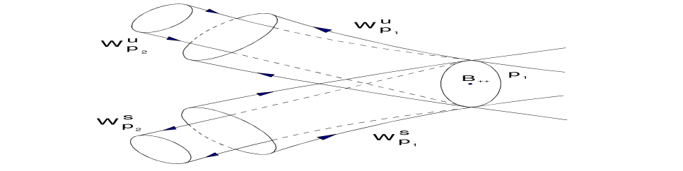
FIG. 2.: Resultant motion from the two directions sketched in the previous figure. ${\rm W}^{U}_{P_{1}}$ stands for unstable manifold for the periodic orbit $p_{1}$ around the fixed point $B_{++}$, while ${\rm W}^{S}_{P_{1}}$ stands for the stable one.

C Numerical results

We have chosen the section $\phi=0$, $\dot{\phi}>0$. In Fig. 3(a) we can see this section for $E=0.3$, below the energy threshold, which is $E_{B}=0.5$ for $m=1.0$. The trajectories are all in KAM tori with a very thin stochastic layer caused by the main separatrix. In Fig. 3(b) the same section is shown for $E=0.511758756$. We can observe a large number of islands due to resonances and a larger chaotic area near the main separatrix. We also point out the gap in the KAM tori which occurs around $a=0$ and $p_{a}=\pm 0.7$, approximately. We shall shortly see how they are filled.

In Fig. 4 we can see part of the center manifold which contains the fixed point $B_{++}$. From each of these periodic orbits the unstable cylinder emanates, and the stable one has these orbits as their asymptotic limit as $\eta\rightarrow\infty$. As mentioned above, these orbits have been obtained by numerical continuation. Figure 5 shows the projection of large periodic orbits onto the $(a,p_{a})$ plane. In fact, they get larger and larger and seem to approach the collapse as the energy increases.

From the fixed point of periodic orbits in the Poincaré section we can globalize the stable and unstable manifolds of the corresponding periodic orbit. In Fig. 6 we show a trajectory bouncing seven times between the the neighborhood of a periodic orbit (p.o.) around $B_{-+}$ and that of the p.o. around $B_{+-}$, before escaping through the unstable manifold of the former. Orbits like that are necessary to numerically find whether the manifolds meet tangentially (integrable case) or if they meet at heteroclinic or homoclinic connections.

Part of the globalized cylinders are shown in Fig. 7, where we show a three-dimensional picture in the variables $(a,\phi,p_{a})$. We have stopped the iteration at the first intersection with the Poincaré section $\phi=0$ ($\dot{\phi}>0$). Note that we have not shown the portions of the unstable and stable manifolds which escape to (or come from) infinity to avoid cluttering the picture. For this same reason we exhibit just a few orbits on each manifold. We can clearly see the four intersections of the cylinders: the unstable (stable) cylinder to $p.o._{B_{++}}$ with the stable (unstable) one to $p.o._{B_{--}};$ the same for $p.o._{B_{+-}}$ with $p.o._{B_{-+}}$ — where $p.o._{B_{i}}$ stands for periodic orbit around the fixed point $B_{i}$. We note that only two of the four intersections belong to the same Poincaré section. To see the other pair, one should just take the oposite sign ($\dot{\phi}<0$).

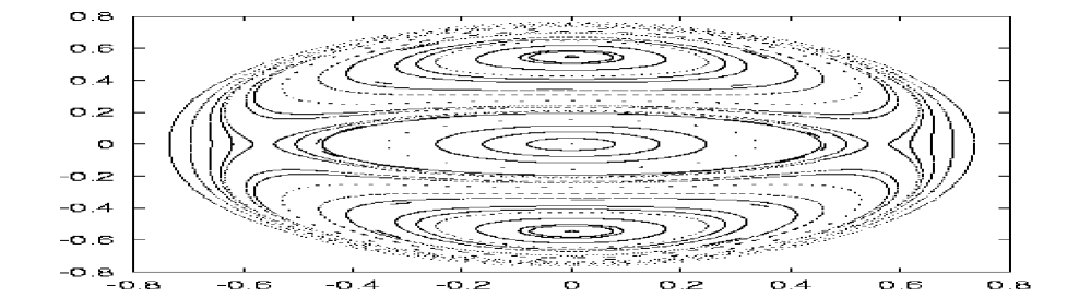
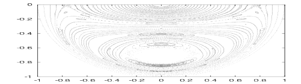
FIG. 3.: Poincaré section $\phi=0$, $\dot{\phi}>0$. (a) $E=0.3<E_{B}$; (b) $E=0.511756758$, only $0.1$ larger than the energy threshold. The upper half is a reflexion around the $p_{a}=0$ axis. Note the gap in the KAM structure around $a=0$ and $p_{a}=\pm 0.7$, approximately.

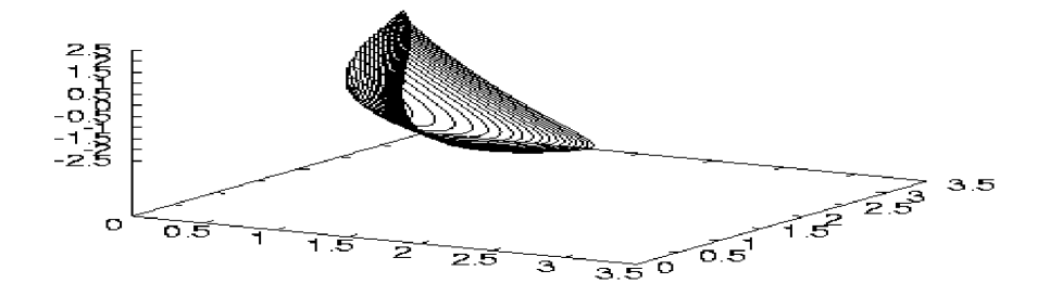
FIG. 4.: Periodic orbits, projection $(a,p_{a},p_{\phi})$, for increasing values of their energies, around the fixed point $(a,\phi)=(1.0,1.0)$.

FIG. 5.: The $(a,p_{a})$ projection of some very large orbits. We believe that they go asymptotically to collapse.

FIG. 6.: An orbit started on the unstable manifold of the $p.o._{B_{+-}}$ approaching the $p.o._{B_{-+}}$ (front-right) making seven universe cycles on the process and finally escaping though the unstable manifold of $p.o._{B_{-+}}$.

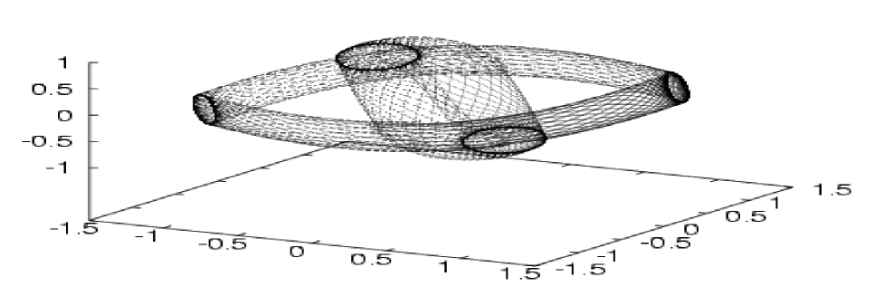
FIG. 7.: We can see the four periodic orbits around the fixed points $B_{i}$ and their respective (un)stable manifolds. They intercept the Poincaré section $\phi=0$ $(\dot{\phi}>0)$, which is a symmetry plane. We stress that the cylinders which come or go to infinity are not shown to avoid cluttering.

As is well known, if the stable and unstable manifolds intersect each other once, they must intersect each other an infinite number of times. Since each such crossing is invariant, their intersections must stay on those cylinders upon both forward and backward iterations of the dynamics. Therefore, they are biasymptotic to the p.o.’s. The Poincaré map of the heteroclinically connecting trajectories initially evolving, say, on the unstable manifold, will then follow the stable one, and from then on it will approach the p.o. around the opposite (w.r.t. the origin) fixed point as $\eta\rightarrow\infty$. On the other hand, as $\eta\rightarrow-\infty$ the trajectory travels towards the original fixed point (of the original p.o.). However, the heteroclinic trajectory itself has to pass through all these points, making then an infinite number of universe cycles and taking an infinite time to do so. To describe the dynamics of a heteroclinic Poincaré iterate is very difficult, let alone four heteroclinic orbits traversing in the same region. However, we can show that trajectories in the neighborhood of the cylinders may, after some universe cycles, go either to collapse or escape to infinity, strongly depending, in an unpredictable way, on their initial conditions. In Fig. 8 we exhibit an orbit starting on the unstable manifold of $p.o._{B_{++}}$ and performing 29 universe cycles before it escapes through the unstable manifold of $p.o._{B_{--}}$ (note the darker line on the left bottom manifold). In Fig. 9 we show another example, where an orbit makes four universe cycles and finaly escapes to infinity (this part of cylinders are not shown to avoid cluttering). In Figures 10(a) and 10b, for $E=0.7307128$ and $E=1.09004$ respectively, we show fourty orbits starting on the unstable manifold of $p.o._{B_{--}}$ and either recollapsing or escaping towards $a\rightarrow\infty$. The presence of the heteroclinic connections, as seen above, unquestionably assures that such a system is chaotic.

Before going to the next aspect of the dynamics, we shall analyse another piece of infomation that can be extracted from Figures 10(a) and 10(b): the lower energy orbits escape only through the symmetrical point with respect to their initial conditions, while some orbits at higher energies escape also through the transverse connections. This can be developed into a tool for reckoning the escape rate noncollapsing universes (i.e., those which do not cross $a=0$ or $\dot{a}>0$).

FIG. 8.: The periodic orbits around $B_{++}$ and $B_{--}$ with the corresponding unstable and stable cylinders which escape to (or arrive from) infinity. The orbit shown starts on the unstable manifod near $B_{++}$ and escapes through the unstable manifold of $B_{--}$ after 29 universe cycles.

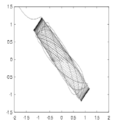
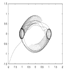
FIG. 9.: In both figures we show part of the stable and the unstable manifolds to the periodic orbits at $E=0.56255168$. Left: The projection onto configuration space of a trajectory starting near the crossing of the unstable manifold of $B_{+-}$ with the stable one from $B_{-+}$. After four cycles it finally escapes to infinity near $B_{-+}$. Right: the projection onto the $(a,pa)$ plane.

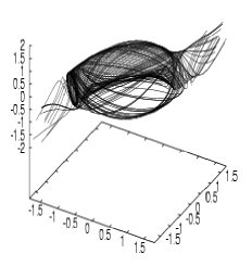
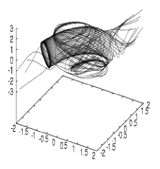
FIG. 10.: Left: Forty escaping or recolapsing trajectories $(a,\phi,p_{a})$ starting on the unstable manifold with $a<0$ (near the $p.o._{B_{-+}}$) for $E=0.7307128$. Right: the same for $E=1.09004$. All orbits were allowed four passages through the Poincaré section.

Another interesting feature is how the heteroclinic cuts blend with cuts of KAM tori and irregular regions.

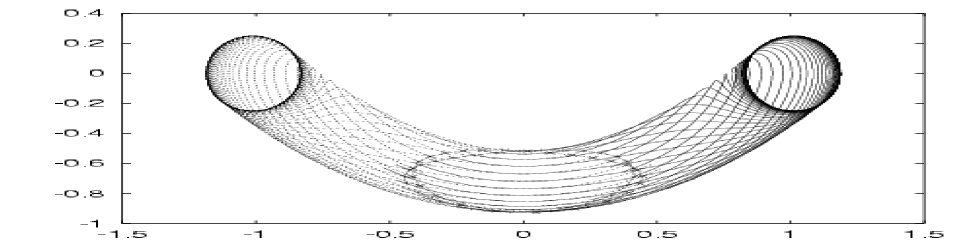
FIG. 11.: Poincaré section and projection of the unstable manifold of $p.o._{B_{++}}$ and the stable manifold of $p.o._{B_{--}}$. The four intersections of the Poincaré section is enhanced with help of lines.

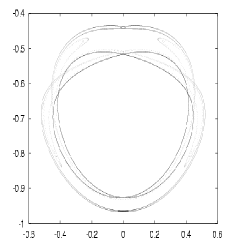
FIG. 12.: (a) Same as Fig. 11 with 1000 initial contiditions showing the first cut of the unstable manifold of $p.o._{B_{++}}$ and the stable one of $p.o._{B_{--}}$; (b) Same as (a), adding the iterates of the second passage through the Poincaré section (10000 initial conditions).

Figure 11 shows the unstable manifold of $p.o._{B_{++}}$ and the stable manifold of $p.o._{B_{--}}$ projected in the plane of the Poincaré section $(a,p_{a})$. In this same picture we show the points (crosses) where those manifolds cut the section. The lines joining them are drawn just to help visualization. In Fig. 12(a) we show the first two cuts (one from each manifold) with a large number (1000) of initial conditions so that the section looks like a continuous curve. The existence of four heteroclinic connections can be easily seen. Figure 12(b) shows two consecutive cuts of each manifold with an even larger (10000) number of points. This increase is necessary because the initial cuts evolve to highly convoluted ones due to the folding and stretching of the cylinders. To follow this picture in detail is beyond the scope of this work. We now superpose the Figs. 3(b) and 12 and find that the heteroclinic cuts are embeded among the tori in the upper and lower part of their Poincaré section, exactly in the gaps that we showed in Fig. 3b. Then, besides the breaking of KAM tori due to the resonances of their frequencies, for $E>E_{B}=0.5$, they are also eroded by the unstable and stable manifolds of the periodic orbits with the same energy. This can be seen clearly in Figure 13. For the sake of clearness, we show the complete lower part ($p_{a}<0$) and only the heteroclinic cuts for the upper part (due to the cylinders of $p.o._{B_{+-}}$ and $p.o._{B_{+-}}$). They merge nicely with the KAM sections and are another source of destruction of regular behaviour.

In Fig. 14 we show a more detailed view of the merging for the energy $E=0.511758762$. There are islands lodged among the cuts of the cylinders (top and bottom): they manage to avoid escaping and are bound to recollapse. We show a particular trajectory corresponding to one of these islands in Fig. 15(a). The empty regions at both right and left of Figure 14 belong to the section with oposite crossing sign. The orbit shown in Fig. 15(b) confirms this hypothesis: they traverse from the neighborhood of $B_{+-}$ and $B_{-+}$. It is interesting how these orbits avoid escaping due to a resonance between $\dot{a}$ and $\dot{\phi}$. Note that both orbits get very near the unstable periodic orbits.

We show in Fig. 17a-b how the KAM tori are squeezed near the trivial fixed point $(0,0)$ as the energy increases, and are finally completely destroyed by the (un)stable manifolds. In Fig. 17(a) we show the section for $E=0.886408856$ where a tiny region near the trivial fixed point still presents KAM tori. As the cylinders expand, the trival fixed point bifurcates. This bifurcation also happens in the real counterpart, as expected; we will postpone this dicussion until the next section.

Another interesting aspect of the imaginary dynamics is a $2$:$1$ bifurcation at $E=1.157691425$. This kind of bifurcation is typical of mappings which are nearly integrable and, at some distance of the equilibrium point, looses its twist character (see Ref. [6] for details). In our case, though, it is more important to stress that this bifurcation creates a region in which tori starting at $a>0$ ($a<0$) stay at the same side of the $a=0$ axis. These noncollapsing universes are shown in Figs. 16. Its bottom right panel shows the small island where the universes are confined to. Note that in the bottom left panel (same figure) the corresponding region is empty since we have given initial conditions with $a>0$. That empty region can only be filled with iterates of trajectories starting at $a<0$, in that range.

As the energy inceases, this structure grows and is pushed away to higher mean values of the radius. In Figs. 17(b) and 17(c), we show the KAM structure left. Note in Fig. 17(b) that the intercepting curves, formed by the iterates of the Poincaré section of the cylinders, squeeze down the amplitude of the momentum $p_{a}$ of the remnant KAM tori, and out from the central region. Another zoom into the black spot of Fig. 17(c) shows a further bifurcation, where the stable periodic orbit becomes unstable yielding two stable ones (the central points in the section). For even larger values of the energy, they finally disappear completely and the (un)stable manifolds will be the only remaining invariant surfaces with the unstable periodic orbits typical of a horse-shoe structure occupying the whole phase space. This is a mechanism by which orbits born close to the singularity may find its way either to infinity or to collapse in an unpredictible way. Other orbits would be trapped as heteroclinic ones approaching one of the stable periodic orbits at $a>0$ having an infinite period (see Fig. 18).

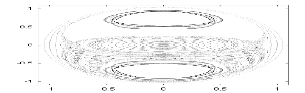
FIG. 13.: Poincaré section of the cylinders and KAM tori for $E=0.562551684$, same as Fig. 17. Universes which before were bound to do only cycles can now find a way to scape to infinity.

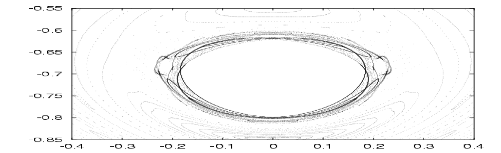
FIG. 14.: Detail of Poincaré section of the cylinders and KAM tori for $E=0.511758756$. Note, at top and bottom, trapped islands among the five cuts of the cylinders, and the gaps at left and right.

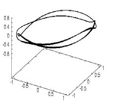
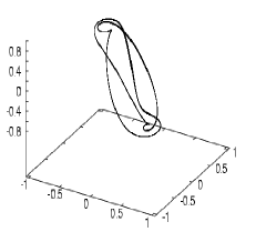
FIG. 15.: Left: The projection onto $(a,\phi,p_{a})$ of a trajectory lodged among the cuts at top and bottom of the previous figure. Right: the same projection of a KAM torus which in the section $\phi<0$ would occupy the gaps on both sides of Fig. 14 (see the text for explanation).

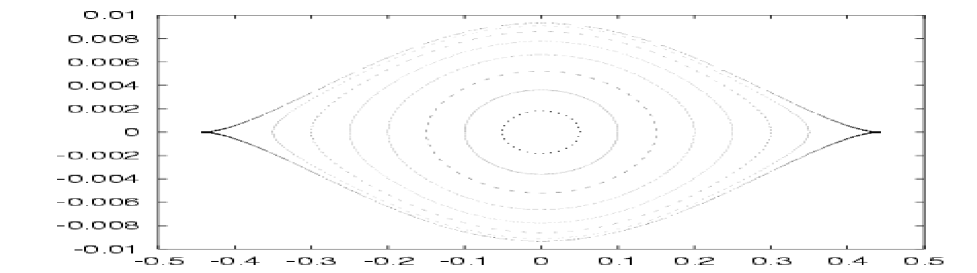
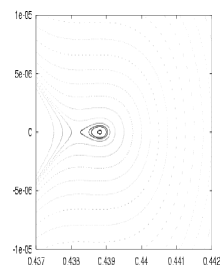
FIG. 16.: The bifurcation at $E=1.15769143$ where the first noncollapsing universes are born. The KAM structure shown in the previous figure originates from this bifurcation. It has been pushed away by the expanding (un)stable manifolds.

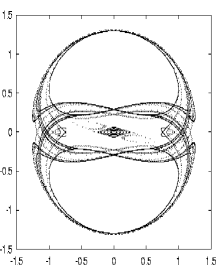
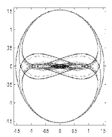
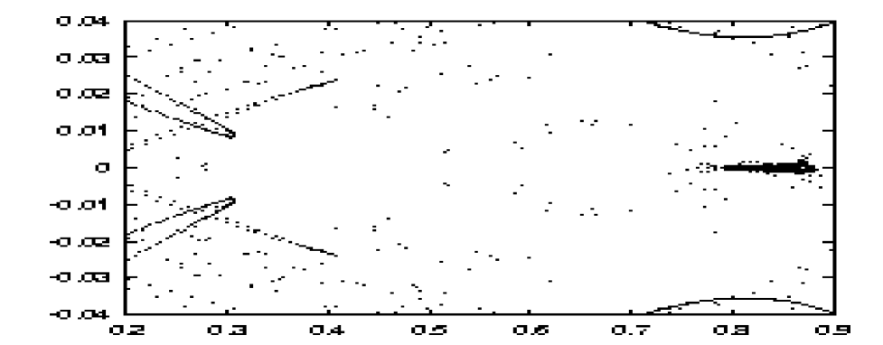
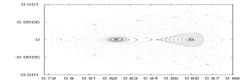
FIG. 17.: Two iterates of the stable and unstable manifolds to a large periodic orbit of $B_{++}$ for $E=0.886408856$ and $E=1.19549093$, respectively. In the bottom, we zoom in the latter to show a detail of the remnant tori structure squeezed between the (un)stable manifolds. Note the axis range of another zoom into what looks like a black spot in the previous magnification.

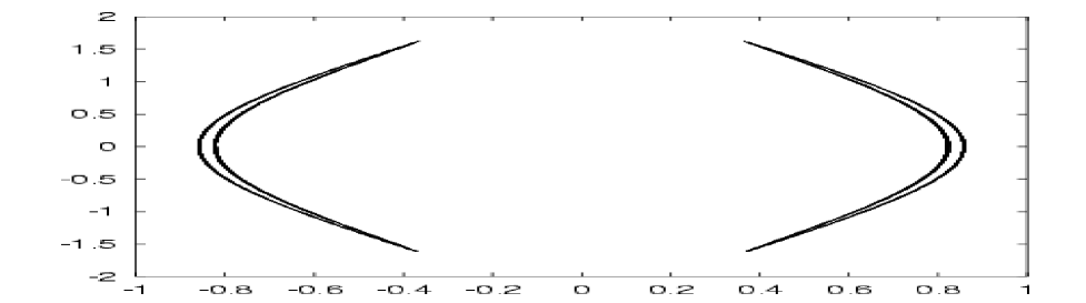
FIG. 18.: Projection onto the configuration space of two tori which stay at the same side of the axis $a=0$. These orbits belong to the remnant structure shown in Fig. 9(c) at $E=1.195549093$.

IV Real problem

We recall the real Hamiltonian:

$$2H=(p_{\phi}^{2}+\phi^{2})-(p^{2}_{a}+a^{2})+m^{2}a^{2}\phi^{2}+\rho_{r}=0.$$ (7)

Since there is a bifurcation of the shared fixed point at the origin in the imaginary case, leading to a noncollapsing KAM structure, we now investigate the real model numerically. As before, for lower energy, the whole energy space is almost integrable, in the sense that eventual resonances (or islands) are very thin structures. As the energy increases, bifurcations become more frequent and for $E=0.5$ the outer tori are completely destroyed while the inner core is kept regular. This is shown in Fig. 19, where we display some sections through $\phi=0$ ($\dot{\phi}>0$) for increasing values of the energy.

For $E\approx 1.16335949$, the trivial fixed point bifurcates from stable to unstable, giving birth to two stable periodic orbits, as shown in Fig. 20. This feature is, of course, shared by the analytical extension as mentioned in the previous section. In Fig. 21 we show 20 iterates of the stable and unstable manifolds. Note how they form intercepting loops which approach the origin, leaving no room for regular motion around the trivial fixed point: the real model is simply obliged to bifurcate. This is the origin of the chaos at large in the analytical extension. However, as we shall see, this bifurcation favors some regularity and noncollapsing KAM structures.

The newborn periodic stable orbits and surrounding KAM tori do not collapse. Two of such tori are seen in Fig. 22 below. The orbit shown in the left of this figure is very near the newborn stable periodic orbit at the bifurcation energy.

FIG. 19.: The outer region becomes irregular as the energy increases. From left to right: $E=0.0$ and $0.3$. Chaos appears in the outer region of the phase space when it opens up and trajectories can escape to infinity performing larger and larger cycles. Note that the six islands belong to two different tori; they were drawn with different initial conditions to enhance this fact.

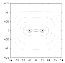
FIG. 20.: Two stable periodic orbits are born at the bifurcation of the trivial fixed point, and the latter becomes unstable. For $E=1.164$ the region of noncollapsing orbits is still very small. On the right figure we show $E=1.3$: the outer layer collapses after more 900 Poincaré iterates, shown by crosses.

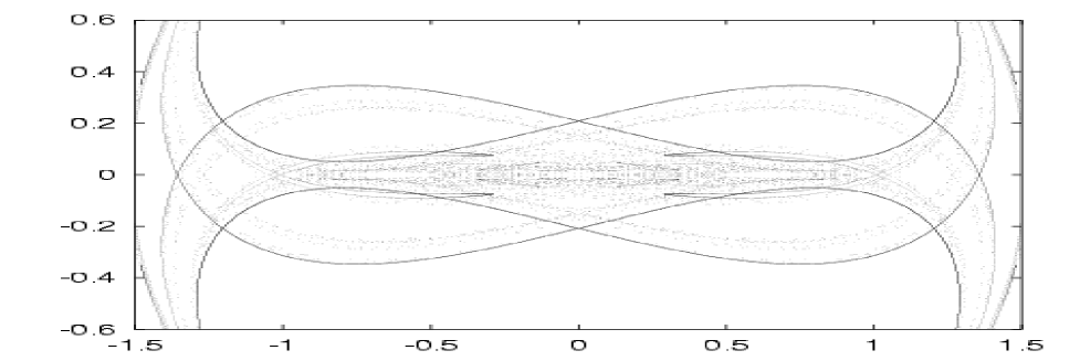
FIG. 21.: We show 20 passages of the stable and unstable manifolds of the analytical continuation for $E=1.16682669$. Note how the origin is gradually surrounded by the intercepting loops of these manifolds.

We have characterized this family of noncollapsing periodic orbits (Fig. 23). It presents three main features: (i) Right after the bifurcation, the solutions present a small value for the maximum scale factor ($a_{max}\ll 1$), but a much higher $\phi$. (ii) A $2$:$1$ resonance between the $a$ and $\phi$ modes (Fig. 24); (iii) As the energy increases, the scale factor oscillates around higher mean values with decreasing amplitude (Fig. 25), while its conjugated momentum reaches a finite maximum amplitude. The amplitude of the $\phi$ field, on the other hand, is just slighlty reduced, while its momentum is largely amplified. The KAM tori around this family of periodic orbits undergoes various bifurcations as the energy increases.

One of these bifurcations is shown in Fig. 26(a), $E=5.0$, where we can see five islands generating a very large stochastic zone. Fig. 26(b) exhibits a very thin noncollapsing tori of period 5. We have not systematically investigated the width of the region of noncollapsing trajectories, but it seems that as the energy increases the region becomes more stable and grows proportionally to the energy. This can be seen in Fig. 27(a), 27(b) and 27(c) for $E=15.0$, $E=50.0$ and $E=200.0$, respectively. We conjecture that the islands become of increasingly higher order and are located at the border of the noncollapsing region. As shown in Fig. 20, the universe sticks to the islands for a long period of time before collapsing – in this particular case, it took $900<i_{c}<950$ Poincaré iterates. The effects of chaos can indeed be observed before the collapse.

FIG. 22.: Two noncollapsing tori for $E=1.164$ and $E=1.125$.

FIG. 23.: Periodic orbits: (left) $a\times p_{a}$; (right) $\phi\times p_{\phi}$.

V Conclusions

The complexification of the phase space allowed us to probe the (otherwise) complex fixed points. Their saddle-center structure is actually responsible for the chaotic behavior previously described in Ref. [7]. Due to the existence of heteroclinic connections in the system, one cannot say if a given trajectory will collapse or escape to infinity.

The most important outcome of our procedure is to discover that, as the origin is reached by the heteroclinic intercepting loops of the stable and unstable manifolds in the analytical continuation, a bifurcation is created at that point, both in the extension and in the real counterpart. We have also shown that, as a consequence, there are KAM structures formed by trajectories which will never collapse after $E=1.16335949$, and they are persistent to very high values of the energy.

FIG. 24.: A three-dimensional plot ($a\times\phi\times p_{\phi}$) of the periodic orbits bifurcated at $E-1.16335949$ showing the 2:1 relation between the $a$ and $\phi$ modes.

FIG. 25.: Range of oscillation of the scale factor $a$ and $\phi$ (symmetric oscillation, $\phi_{min}=-\phi_{max}$, not shown) for increasing energy. The line $\Delta a\equiv a_{max}-a_{min}$ goes asymptotically to zero.

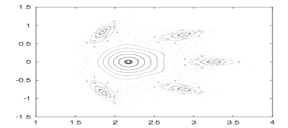
FIG. 26.: The bifurcation at $E=5.0$.

FIG. 27.: The regularity of KAM tori at $E=15.0$, $50.0$, and $200$. We conjecture that there is a bifurcation of higher order at the border of the non-colapsing structure.

VI Acknowledgment

The authors wish to thank Mario B. Matos for interesting discussions. S.E.J. thanks the UFRJ for the kind and warm hospitality, where most of this work was accomplished. We are also indebted to Fundação José Bonifácio (FUJB) for partial computational support. S.E.J. was partially supported by CNPq.

REFERENCES

- [1] K. Ferraz, G. Francisco and G. E. A. Matsas, Phys. Lett. A 156, 407 (1991).
- [2] S. Biswas et al, Gen Relativ. Gravit. 35, 1 (2003); S. Biswas et al, Int. J. Mod. Phys. A 15, 3717 (2000).
- [3] M. V. John and K. B. Joseph, Class. Quantum Grav. 14, 1115 (1997).
- [4] N. J. Cornish and J. J. Levin, Phys. Rev. D 53 3022 (1996).
- [5] A. E. Motter and P. S. Letelier, Phys. Rev. D 65 068502 (2002).
- [6] C. Simó, T. J. Stuchi, Physica D 140 1 (2000).
- [7] E. Calzetta and C. El Hasi, Class. Quantum Grav. 10 1825 (1993); Phys. Rev. D 51 2713 (1995); E. Calzetta, ibid. 63 044003 (2001).
- [8] S. Blanco et al., Gen. Rel. Gravit. 26, 1131 (1994).
- [9] L. Bombelli et al.. J. Math. Phys. 39, 6040 (1998).
- [10] H. P. de Oliveira, I. D. Soares, and T. J. Stuchi, Phys. Rev. D 56 730 (1997).
- [11] M. A. Castagnino, H. Giacomini, and L. Lara, Phys. Rev. D 63 044003 (2001).