Nonradial oscillations of quark stars

Abstract

Recently, it has been reported that a candidate for a quark star may have been observed. In this article, we pay attention to quark stars with radiation radii in the reported range. We calculate nonradial oscillations of $f$-, $w$- and $w_{\rm II}$-modes. Then, we find that the dependence of the $f$-mode quasi-normal frequency on the bag constant and stellar radiation radius is very strong and different from that of the lowest $w_{\rm II}$-mode quasi-normal frequency. Furthermore we deduce a new empirical formula between the $f$-mode frequency of gravitational waves and the parameter of the equation of state for quark stars. The observation of gravitational waves both of the $f$-mode and of the lowest $w_{\rm II}$-mode would provide a powerful probe for the equation of state of quark matter and the properties of quark stars.

I Introduction

Since the 1980s, there have been many studies about objects known as quark stars. If the true ground state of matter is not the nuclear state but a quark state as Witten conjectured Witten1984 , there may exist objects composed of quark matter. For simplicity, the bag model equation of state (EOS) has often been used for studying quark matter. Lattimer and Prakash calculated stellar properties with this EOS Lattimer2001 . In reality, it is quite difficult to determine the EOS of quark matter by experiments on the ground, because quark matter will appear at extremely high density. In this respect, the observation of astrophysical compact objects may be a unique means to determine the equation of state for cold high-density matter Lindblom1992 ; Harada2001 .

Recently, the radiation radius of the compact star RXJ185635-3754 was estimated to be very small ($3.8\mbox{km}\lesssim R_{\infty}\lesssim 8.2\mbox{km}$) based on X-ray observations by Chandra Drake2002 . The radiation radius is related as $R_{\infty}\equiv R/\sqrt{1-2M/R}$ to the areal radius $R$ and mass $M$ of the star. This compact star is too small to construct with the normal EOS’s which are currently adopted for neutron stars Lattimer2001 . This star should be a candidate for a quark star. Inspired by this observation, Nakamura proposed several scenarios about the formation of quark stars Nakamura2002 .

However, it should be noted that there exist many subsequent articles which question the whole observation. For example, Pons et al. pointed out, by employing the data of not only X-ray observation but also UV/optical observation, that if RXJ185635-3754 is represented by the simplest uniform-temperature heavy-element atmospheric model, this compact star has $R_{\infty}\approx 8$km, $M\approx 0.9M_{\odot}$ and $R\approx 6$km Pons2002 . Though this radiation radius is included in the range suggested by Drake2002 , these properties can not be constructed, even if the quark matter EOS is used.

If a compact object oscillates for some reason, gravitational waves are emitted from the object. The trigger of the oscillation may be a nonspherical supernova explosion, coalescence with another compact object, violent mass influx due to possible instability of the surrounding accretion disk, and so on. The oscillations damp out because the gravitational waves carry away oscillational energy. So these oscillations are called quasi-normal modes (QNMs). If the gravitational waves from a compact object are detected, we can get information about the source object.

Gravitational wave observation projects, such as LIGO Althouse1992 , VIRGO Giazotto1990 , GEO600 Hough1996 and TAMA300 Tsubono1995 , are making remarkable progress in sensitivity. Among them, TAMA300, GEO600 and LIGO are now in operation. If highly sensitive gravitational wave detectors are available, we may obtain a large amount of data for frequencies and damping times of gravitational waves emitted from compact objects. The systematic study of gravitational wave modes leads to the so called “gravitational wave asteroseismology”, which has been initiated and being presented by various authors (see Andersson1996 ; Andersson1998 ; Kokkotas1999 ; KokkotasAndersson2001 ; Kokkotas2001 ). If we have a good empirical formula for gravitational wave oscillational frequencies and damping times as functions of stellar properties, it will be very useful in obtaining information for source stars from gravitational wave observations. In this context, Andersson and Kokkotas calculated QNMs with various EOSs and proposed an empirical formula between the QNMs and properties of neutron stars Andersson1996 ; Andersson1998 . Kokkotas, Apostolatos and Andersson improved this empirical formula by one which included the relevant statistical errors Kokkotas2001 . These works treated the polar modes of oscillation and the results are well summarized in Kokkotas1999 ; KokkotasAndersson2001 . Benhar, Berti and Ferrari calculated axial modes and showed that the axial mode gives more direct and explicit information on the stiffness of EOS compared to the polar mode Benhar2000 . All these works are for normal neutron stars, i.e., assuming normal equations of state for nuclear matter.

On the other hand, Yip, Chu and Leung studied nonradial stellar oscillations of quark stars whose radii are around 10 km Yip1999 . However, the reported radius of the star RXJ185635-3754 is much smaller than the radii of the stellar models examined by Yip, Chu and Leung. In this paper, we calculate nonradial oscillations of quark stars whose radiation radii are in the range of $3.8\mbox{km}\lesssim R_{\infty}\lesssim 8.2\mbox{km}$, and examine the relation between the QNMs of quark stars and the EOS of quark matter. Our main concern in this article is whether one could distinguish the EOS of quark matter by the direct detection of the gravitational wave.

QNMs are classified into two classes. One is a class of fluid modes, which mainly couple with the stellar fluid, while the other is one of spacetime modes which are connected with spacetime oscillation, which couple mainly to metric perturbations. Non-rotating stars admit fluid modes only for polar perturbations. The most widely studied fluid modes are $f$-, $p$- and $g$-modes Andersson1998 ; Sotani2001 . The $f$-mode is the fundamental mode. There is only one $f$-mode for each $l$. The $p$-mode is the pressure mode which arises from fluid pressure. The $g$-mode is the gravity mode which is caused by buoyancy due to density discontinuity and/or the temperature gradient of stars and other factors. The damping rates of these fluid modes are very small compared with the frequency. The spacetime modes include $w$- and $w_{\rm II}$- modes Kokkotas1992 ; Leins1993 . The damping rate of $w$-modes is comparable to the frequency. For each stellar model, there are found one or a few $w_{\rm II}$-modes, whose complex frequency is located near the imaginary axis. Here we deal with only polar perturbation because our main concern is the relationship between the gravitational waves and EOS. For simplicity, we pay attention here only to $f$-, $w$- and $w_{\rm II}$-modes. Recently, Kojima and Sakata calculated the $f$-mode quasi-normal frequency for quark star models, and pointed out the possibility of distinguishing between quark stars and neutron stars by detecting both the $f$-mode frequency and damping rate Kojima2002 .

The plan of this paper is as follows. We present basic equations to construct quark stars and show the properties of quark star structure in Sec. II. In Sec. III, we present the equations and method to determine the QNMs for spherically symmetric stars, show numerical results for the quasi-normal frequencies of quark-star models constructed in Sec. II, and discuss their implications. Moreover, we apply the empirical formula proposed by Kokkkotas et al. to quark star models and deduce a new empirical formula from our numerical results between the $f$-mode frequency of the gravitational wave and the parameter of EOS in Sec. IV. We conclude in Sec. V. We adopt the unit of $c=G=1$, where $c$ and $G$ denote the speed of light and gravitational constant, respectively, and the metric signature of $(-,+,+,+)$.

II Structure of Quark Stars

We consider a static and spherical star. For this case, the metric is described by

$$ds^{2}=-e^{2\Phi}dt^{2}+e^{2\Lambda}dr^{2}+r^{2}\left(d\theta^{2}+\sin^{2}\theta d\phi^{2}\right),$$ (1)

where $\Phi,\Lambda$ are metric functions of $r$. The mass function $m(r)$ is defined as

$$m(r)=\frac{1}{2}r\left(1-e^{-2\Lambda}\right).$$ (2)

This mass function satisfies

$$\frac{dm}{dr}=4\pi r^{2}\rho,$$ (3)

where $\rho$ is the energy density. The equilibrium stellar model is derived by solving the Tolman-Oppenheimer-Volkoff equation,

$$\frac{dP}{dr}=-\frac{\left(\rho+P\right)\left(m+4\pi r^{3}P\right)}{r\left(r-2m\right)},$$ (4)

where $P$ is the pressure of the fluid, and the potential $\Phi$ is given by

$$\frac{d\Phi}{dr}=\frac{\left(m+4\pi r^{3}P\right)}{r\left(r-2m\right)}.$$ (5)

For solving these equations, we need an additional equation, i.e., the equation of state.

Though a quark star may be either a light quark star made up of $u$ and $d$ quarks or a strange quark star composed of a mixture of $u$, $d$ and $s$ quarks, we construct simple models by using the bag model EOS, which neglects the masses of $u$ and $d$ quarks. This bag model EOS is characterized by three parameters: the strong interaction coupling constant $\alpha_{c}$, the bag constant $B$ and the mass $m_{s}$ of the $s$ quark. The dependence of stellar properties on the bag constant is much stronger than that on $\alpha_{c}$ and $m_{s}$ Kohri2002 . In this paper we use the bag model EOS derived for a massless strange quark,

$$P=\frac{1}{3}(\rho-4B).$$ (6)

The bag constant $B$ is a positive energy density, which corresponds to latent heat. The stellar radius $R$ is defined as the position where the pressure is zero. At the surface, the density profile is discontinuous. Although the value of the bag constant, which is a phenomenological parameter, should be determined by the underlying strong interaction dynamics, it is difficult to determine this value from our present understanding of QCD. However, if strange quark matter is the true ground state, the energy of this true ground state per particle would not be over the nucleon mass 939 MeV at baryon density for zero pressure matter. This constraint implies a maximum value of the bag constant $B$ as follows Prakash1990 :

$$B\leq B_{\text{max}}=94.92\left(1-\frac{2\alpha_{c}}{\pi}\right)\text{MeV fm}^{-3}.$$ (7)

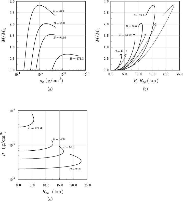
Figure 1: Relations (a) between mass $M$ and central density $\rho_{c}$, (b) between $M$ and radius $R$ (solid line) and between $M$ and radiation radius $R_{\infty}$ (broken line), and (c) between “average density” $\bar{\rho}\equiv 3M/4\pi R^{3}$ and radiation radius $R_{\infty}$ of quark stars for four values of the bag constant, $B=28.9\mbox{MeV fm}^{-3}$, $56.0\mbox{MeV fm}^{-3}$, $94.92\mbox{MeV fm}^{-3}$ and $471.3\mbox{MeV fm}^{-3}$.

For definiteness, we use three values of the bag constant, $B=28.9$, $56.0$ and $94.92$ MeV fm^-3. Although $B_{st}^{1/4}=145$ MeV or $B_{st}=57.8$ MeV fm^-3 has been often used for the study of quark-gluon plasma so far, we adopt $B=56.0$ MeV fm^-3 to compare with the results in Yip1999 . The other values of the bag constant are the maximum value for $\alpha_{c}=0$ and half the standard value $B_{st}$. We show the mass $M$ of quark stars as a function of the central density $\rho_{c}$ for these three values of the bag constant in Fig. 1(a), the relations between $M$ and $R$ and between $M$ and $R_{\infty}$ in Fig. 1(b), and the relation between “average density” $\bar{\rho}\equiv 3M/4\pi R^{3}$ and $R_{\infty}$ in Fig. 1(c). These figures are plotted for $4B<\rho_{c}\leq 5.0\times 10^{15}$ g/cm^-3. The radiation radius may be determined from X-ray observations such as Drake2002 . We pay attention to the stars whose radiation radii are in the range of $3.8-8.2$ km. In this range of radiation radius, we pick up three values, $R_{\infty}=3.8$, $6.0$ and $8.2$ km.

On the other hand, Nakamura argued that the mass of the compact star reported in Drake2002 should be roughly $0.7M_{\odot}$ in order to account for its observed X-ray luminosity Nakamura2002 . If we use a value smaller than $B_{\text{max}}$, however, the mass of a quark star whose radiation radius is in the range of $3.8-8.2$ km is far below $0.7M_{\odot}$ as seen in Fig. 1(b). Therefore he pointed out the possibility of adopting the value $B=471.3$ MeV fm^-3, which is rather greater than $B_{\text{max}}$. We consider a quark-star mass of $M=0.7M_{\odot}$ for this value of the bag constant to compare with other models. Also for the case $B=471.3$ MeV fm^-3, we plot the relation between $M$ and $\rho_{c}$ in Fig. 1(a), the relations between $M$ and $R$ and between $M$ and $R_{\infty}$ in Fig. 1(b), and the relation between $\bar{\rho}$ and $R_{\infty}$ in Fig. 1(c). In this case, each plot is for $4B<\rho_{c}\leq 5.0\times 10^{16}$ g/cm^-3. The properties of our quark-star models are tabulated in Table 1.

III Nonradial Oscillations of Quark Stars

III.1 Method

The QNMs are determined by solving the perturbation equations with appropriate boundary conditions. The metric perturbation is given by

$$g_{\mu\nu}=g^{(B)}_{\mu\nu}+h_{\mu\nu},$$ (8)

where $g^{(B)}_{\mu\nu}$ is the background metric of a spherically symmetric star (1). We have applied a formalism developed by Lindblom and Detweiler Lindblom1985 for relativistic nonradial stellar oscillations. In this formalism, $h_{\mu\nu}$ for polar perturbations is described as

$$h_{\mu\nu}=\left(\begin{array}[]{cccc}r^{l}\hat{H}e^{2\Phi}&i\omega r^{l+1}\hat{H}_{1}&0&0\\ i\omega r^{l+1}\hat{H}_{1}&r^{l}\hat{H}e^{2\Lambda}&0&0\\ 0&0&r^{l+2}\hat{K}&0\\ 0&0&0&r^{l+2}\hat{K}\sin^{2}\theta\end{array}\right)Y^{l}_{m}\,e^{i\omega t},$$ (9)

where $\hat{H},\hat{H}_{1},$ and $\hat{K}$ are perturbed metric functions with respect to $r$, and the components of the Lagrangian displacement of fluid perturbations are expanded as

$$\xi^{r} = \frac{r^{l}}{r}e^{\Lambda}\hat{W}Y^{l}_{m}\,e^{i\omega t},$$ (10)

$$\xi^{\theta} = -\frac{r^{l}}{r^{2}}e^{\Lambda}\hat{V}\frac{\partial}{\partial\theta}Y^{l}_{m}\,e^{i\omega t},$$ (11)

$$\xi^{\phi} = -\frac{r^{l}}{r^{2}\sin^{2}\theta}e^{\Lambda}\hat{V}\frac{\partial}{\partial\phi}Y^{l}_{m}\,e^{i\omega t},$$ (12)

where $\hat{W}$ and $\hat{V}$ are functions of $r$.

Then the perturbation equations derived from Einstein equations are given by

$$\frac{d\hat{H}_{1}}{dr}=-\frac{1}{r}\left[l+1+\frac{2m}{r}e^{2\Lambda}+4\pi r^{2}(P-\rho)e^{2\Lambda}\right]\hat{H}_{1}$$

$$\hskip 34.14322pt+\frac{1}{r}e^{2\Lambda}\left[\hat{H}+\hat{K}+16\pi(P+\rho)\hat{V}\right],$$ (13)

$$\frac{d\hat{K}}{dr}=\frac{l(l+1)}{2r}\hat{H}_{1}+\frac{1}{r}\hat{H}-\left(\frac{l+1}{r}-\frac{d\Phi}{dr}\right)\hat{K}+\frac{8\pi}{r}(P+\rho)e^{\Lambda}\hat{W},$$ (14)

$$\frac{d\hat{W}}{dr}=-\frac{l+1}{r}\hat{W}+re^{\Lambda}\left[\frac{1}{\gamma P}e^{-\Phi}\hat{X}-\frac{l(l+1)}{r^{2}}\hat{V}-\frac{1}{2}\hat{H}-\hat{K}\right],$$ (15)

$$\frac{d\hat{X}}{dr}=-\frac{l}{r}\hat{X}+(P+\rho)e^{\Phi}\biggl{[}\frac{1}{2}\left(\frac{d\Phi}{dr}-\frac{1}{r}\right)\hat{H}-\frac{1}{2}\left(\omega^{2}re^{-2\Phi}+\frac{l(l+1)}{2r}\right)\hat{H}_{1}$$

$$\hskip 34.14322pt+\left(\frac{1}{2r}-\frac{3}{2}\frac{d\Phi}{dr}\right)\hat{K}-\frac{l(l+1)}{r^{2}}\frac{d\Phi}{dr}\hat{V}$$

$$\hskip 34.14322pt-\frac{1}{r}\left(\omega^{2}e^{-2\Phi+\Lambda}+4\pi(P+\rho)e^{\Lambda}-r^{2}\left\{\frac{d}{dr}\left(\frac{1}{r^{2}}e^{-\Lambda}\frac{d\Phi}{dr}\right)\right\}\right)\hat{W}\biggr{]},$$ (16)

$$\biggl{[}1-\frac{3m}{r}-\frac{l(l+1)}{2}-4\pi r^{2}P\biggr{]}\hat{H}-8\pi r^{2}e^{-\Phi}\hat{X}$$

$$\hskip 34.14322pt+r^{2}e^{-2\Lambda}\left[\omega^{2}e^{-2\Phi}-\frac{l(l+1)}{2r}\frac{d\Phi}{dr}\right]\hat{H}_{1}$$

$$\hskip 34.14322pt-\left[1+\omega^{2}r^{2}e^{-2\Phi}-\frac{l(l+1)}{2}-\left(r-3m-4\pi r^{3}P\right)\frac{d\Phi}{dr}\right]\hat{K}=0,$$ (17)

$$\hat{V}=\frac{e^{2\Phi}}{\omega^{2}(P+\rho)}\left[e^{-\Phi}\hat{X}+\frac{1}{r}\frac{dP}{dr}e^{-\Lambda}\hat{W}+\frac{1}{2}(P+\rho)\hat{H}\right].$$ (18)

In deriving the above equations for perturbations, we assume a perfect fluid. Rigorously speaking, it will not be valid because of the existence of matter viscosity. However, little is known about the viscosity of cold quark matter. Here we omit the viscosity as a possible approximation. In Eq. (15), $\gamma$ is the adiabatic index of the unperturbed stellar model, which is calculated as

$$\gamma=\frac{\rho+P}{P}\frac{dP}{d\rho}=\frac{1}{3}\frac{\rho+P}{P},$$ (19)

where the bag model EOS (6) is used in the second equality. The set of Eqs. (13) $-$ (16) is a set of differential equations connecting the variables $\hat{H}_{1}$, $\hat{K}$, $\hat{W}$ and $\hat{X}$, and Eqs. (17) and (18) are the algebraic equations for the variables $\hat{H}$ and $\hat{V}$. The perturbation equations outside the star are described by the Zerilli equations. By imposing boundary conditions such that perturbative variables are regular at the center of the star, the Lagrangian perturbation of pressure vanishes at the stellar surface, and the gravitational wave is only an outgoing one at infinity, one can reduce this to an eigenvalue problem. The boundary condition at the stellar surface is $\hat{X}=0$, because $\hat{X}\equiv-r^{-l}e^{\Phi}\Delta P$, where $\Delta P$ is Lagrangian perturbation of pressure. Furthermore, we set the term $e^{-\Phi}\hat{X}/\gamma P$ in Eq. (15) to zero at the stellar surface, because $\gamma P=4B/3$ at $r=R$. For the treatment of the boundary condition at infinity, we adopt the method of continued-fraction expansion proposed by Leaver Leaver1985 . The details of the determination of quasi-normal frequencies are given in Sotani2001 .

III.2 Numerical Results

III.2.1 $f$-mode

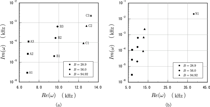
Figure 2: Complex frequencies of $f$-mode for quark stars. The squares, triangles and circles correspond to stars with $B=28.9$ MeV fm^-3, $56.0$ MeV fm^-3, and $94.92$ MeV fm^-3, respectively. In each set, the upper, middle and lower marks are for the cases of $R_{\infty}=8.2$ km, $6.0$ km, and $3.8$ km, respectively. The labels in this figure correspond to the stellar model in Table 1. For (b), the plot for $B=471.3$ MeV fm^-3 is also included as the diamond.

We plot the complex frequencies of the $f$-mode for $l=2$ in Fig. 2. In this figure, the squares, triangles and circles denote the cases $B=28.9$ MeV fm^-3, $B=56.0$ MeV fm^-3 and $B=94.92$ MeV fm^-3, respectively. In each set, the upper, middle and lower marks correspond to the stellar models of $R_{\infty}=8.2$ km, $R_{\infty}=6.0$ km and $R_{\infty}=3.8$ km, respectively. The labels in this figure correspond to those of the stellar models in Table 1.

As can be seen in Fig. 2(a), the $f$-mode frequency depends strongly on the bag constant but very weakly on the stellar radiation radius. This result agrees with that of Kojima and Sakata Kojima2002 . Therefore, if the radiation radius of a quark star is determined by observation, even though the value of the radiation radius is somewhat uncertain, we can directly obtain the value of the bag constant by detecting $f$-mode QNMs (see Sec. IV). Furthermore, we can restrict the mass of the source star by employing the observational value of the radiation radius.

The reason why the $f$-mode frequency depends strongly on the bag constant is understood as follows. The $f$-mode frequency depends strongly on average density but very weakly on the EOS Andersson1998 . In the case of quark stars with small radii, the average density is almost determined by the bag constant alone, as can be seen in Fig. 1(c). Thus, the $f$-mode frequency depends strongly on the bag constant.

Moreover, we can see that the damping rate of the $f$-mode depends on the stellar radiation radius for each bag constant, which also agrees with the result by Kojima and Sakata Kojima2002 . So, if we get data on the damping rate of the $f$-mode by observation, we can determine the stellar radiation radius independently of X-ray observations. However, one must keep in mind that the measurement of frequency is far more accurate than that of damping rate, because the estimated relative error in frequency is about three orders of magnitude smaller than that in damping rate Kokkotas2001 .

The $f$-mode frequency of a quark star with $M=0.7M_{\odot}$ and $B=471.3$ MeV fm^-3 ($N1$) is plotted in Fig. 2(b). In this figure, results for the case $B\leq B_{\text{max}}$ are also plotted for comparison. Compared with the $f$-mode frequencies for $B\leq B_{\text{max}}$, the plot for $B=471.3$ MeV fm^-3 is relatively far away in phase space. This is mainly due to the large difference in the average density of quark stars.

III.2.2 $w$- and $w_{\rm II}$-modes

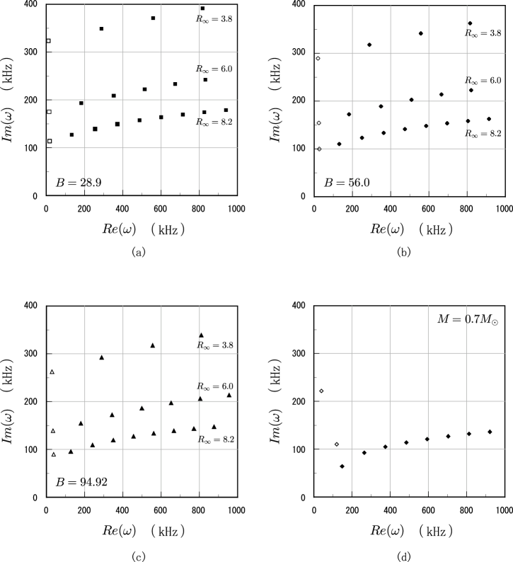
Figure 3: Complex frequencies of both $w$- and $w_{\rm II}$-modes (a) for $B=28.9$ MeV fm^-3, (b) for $B=56.0$ MeV fm^-3, (c) for $B=94.92$ MeV fm^-3, and (d) for $B=471.3$ MeV fm^-3. For (a)-(c), the upper, middle and lower sequences correspond to the quark stars of $R_{\infty}=3.8$ km, $6.0$ km, and $8.2$ km, respectively. For (d), the mass of the stellar model is $0.7M_{\odot}$. Filled and non-filled marks denote $w$- and $w_{\rm II}$-modes, respectively. These stellar models are listed in Table 1.

The calculated complex frequencies of $w$- and $w_{\rm II}$-modes for $l=2$ are plotted in Fig. 3. In these figures, the filled and non-filled marks correspond to $w$- and $w_{\rm II}$-modes, respectively. Figures 3(a), (b) and (c) correspond to $B=28.9$, $56.0$ and $94.92$ MeV fm^-3, respectively. In each figure, the upper, middle and lower sequences correspond to the stellar models of $R_{\infty}=3.8$ km ($A1$, $B1$, $C1$), $R_{\infty}=6.0$ km ($A2$, $B2$, $C2$) and $R_{\infty}=8.2$ km ($A3$, $B3$, $C3$), respectively. In Fig. 3(d), we plot the complex frequencies of $w$- and $w_{\rm II}$-modes of the star of $0.7M_{\odot}$ with $B=471.3$ MeV fm^-3 ($N1$).

In order to obtain the tendency of $w$- and $w_{\rm II}$-modes with changing compactness, we calculate the $w$- and $w_{\rm II}$-modes of the stellar models whose compactness is much larger than that of the stellar models depicted in Figs. 3(a), (b) and (c). From this calculation, we find two $w_{\rm II}$-modes for the stellar model of higher compactness, for example, for $\rho_{c}=1.4\times 10^{15}$ g/cm^-3 with $B=56.0$ MeV fm^-3. In this case, the complex frequencies of $w$- and $w_{\rm II}$-modes appear similarly as in Fig. 3(d). Furthermore, we see that as the compactness of quark star gets smaller, the complex frequencies of the $w_{\rm II}$-modes shift toward the imaginary axis, while both the frequency and damping rate of $w$-modes become slightly larger. If the compactness is very small, the frequencies of $w_{\rm II}$-modes can be too small to find except for the lowest $w_{\rm II}$-mode which has the largest frequency among all $w_{\rm II}$-modes. That is why Figs. 3(a), (b) and (c) are quite different from the results obtained by Yip, Chu and Leung Yip1999 in the location of $w_{\rm II}$-modes.

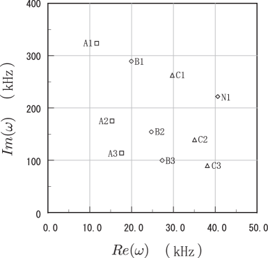
Figure 4: Complex frequencies of the lowest $w_{\rm II}$-mode for each stellar model except for the plot for $B=471.3\mbox{MeV fm}^{-3}$, for which the second $w_{\rm II}$-mode is plotted. The labels in this figure correspond to those of the stellar models in Table 1.

We pick up the lowest $w_{\rm II}$-mode and plot in Fig. 4 for each stellar model. The frequency of the lowest $w_{\rm II}$-mode depends strongly on the bag constant. In this figure, the labels correspond to those of the stellar model in Table 1. Thus, we can get information about the bag constant or the stellar radiation radius by observing the lowest $w_{\rm II}$-mode frequency. Moreover, we could obtain a more stringent restriction by using the damping rate, although it seems more difficult to determine the damping rate by observation as Andersson and Kokkotas mentioned Andersson1996 .

On the other hand, in Fig. 3, we see that both the frequency and damping rate of $w$-modes have little dependence on the bag constant. Therefore it is difficult to determine the value of the bag constant by employing the observation of $w$-modes. In fact, the $w$-mode frequencies are all far beyond the frequency band for which gravitational wave interferometers such as LIGO, VIRGO, GEO600 and TAMA300 have good sensitivity Thorne1998 .

As seen in Fig. 3(d), because the compactness of model $N1$ is much larger than that of the stellar models constructed with $B\leq B_{\text{max}}$, the appearance of the complex frequencies of the $w$- and $w_{\rm II}$-modes is quite different from that for the case of $B\leq B_{\text{max}}$. In Fig.4, we also plot the $w_{\rm II}$-mode complex frequency closest to the imaginary axis among the $w_{\rm II}$-modes previously found for model $N1$. From this result, we see that if the bag constant is too large, or is as large as the one adopted by Nakamura, it may be difficult to distinguish between the lowest $w_{\rm II}$-mode for the case of $B\leq B_{\text{max}}$ and one which is closest to the imaginary axis for the case of $B=471.3$ MeV fm^-3. In respect of this problem, even if we cannot distinguish between the lowest $w_{\rm II}$-mode for the case of $B\leq B_{\text{max}}$ and one which is closest to the imaginary axis for the case of $B=471.3$ MeV fm^-3, it may be possible to discriminate between these two kinds of $w_{\rm II}$-modes by employing the observed $f$-mode frequency, because the plot of $f$-mode for $B=471.3$ MeV fm^-3 is relatively far away in phase space, compared with the $f$-mode frequencies for $B\leq B_{\text{max}}$.

IV Empirical formula

Kokkotas, Apostolatos and Andersson constructed the empirical formulas for $f$-mode of neutron stars Kokkotas2001 ;

$$\frac{Re(\omega)}{1\text{kHz}} \cong 2\pi\,\left[(0.78\pm 0.01)+(1.63\pm 0.01)\left(\frac{M}{1.4M_{\odot}}\right)^{1/2}\left(\frac{10\text{km}}{R}\right)^{3/2}\right],$$ (20)

$$\frac{Im(\omega)}{1\text{Hz}} \cong 2\pi\,\left(\frac{M}{1.4M_{\odot}}\right)^{3}\left(\frac{10\text{km}}{R}\right)^{4}\left[(22.85\pm 1.51)-(14.65\pm 1.32)\left(\frac{M}{1.4M_{\odot}}\right)\left(\frac{10\text{km}}{R}\right)\right].$$ (21)

We apply these empirical formulas to quark star models, and show the results in Table 2. As seen these results, though these formulas are deduced by employing various EOS including the realistic one for neutron stars, it is found that a simple extrapolation to quark stars is not very successful. We try to construct the alternative formula for quark star models by using our numerical results for $f$-mode QNMs, but we can not do this using the same method as Kokkotas et al., because some special relation between $f$-mode QNMs and the stellar properties can not be found.

In the previous section, we see that the $f$-mode frequency depends strongly on not the stellar radiation radius but the bag constant. So, in order to get the relationship between $f$-mode frequency $Re(\omega)$ and the bag constant $B$, we calculate $f$-mode QNMs emitted by six more stellar models in addition to the above nine stellar models (A1$\sim$A3, B1$\sim$B3, C1$\sim$C3). The radiation radii of these six added models are fixed at $R_{\infty}=3.8$, $6.0$ and $8.2$ km, and the adopted bag constants are $B=42.0$ and $75.0$ MeV fm^-3. The results of calculation are plotted in Fig. 5, and listed in table 3. In Fig. 5, squares, triangles and circles correspond to the stellar models whose radiation radii are fixed at $3.8$, $6.0$ and $8.2$ km, respectively. From our numerical results, we find the following new empirical formula between the $f$-mode frequency $Re(\omega)$ and the bag constant $B$:

$$\frac{Re(\omega)}{1\text{kHz}}\,\approx 1.173\times\left(\frac{B}{1\text{MeV fm}^{-3}}\right)^{0.5252}.$$ (22)

This empirical formula is also shown with a dotted line in Fig. 5. In Table 3, we listed the bag constant which is obtained by substituting the given $f$-mode frequencies into the empirical formula (22), and its deviation from the true value. Here we calculate the deviation as

$$\frac{B-B_{emp}}{B},$$ (23)

where $B$ and $B_{emp}$ are the bag constant we adopted for calculation of QNMs and the one given by substituting the $f$-mode frequency into the above empirical formula, respectively. We see that this empirical formula is very useful, because it is possible to determine the bag constant precisely by employing the observation of $f$-mode frequency, even if the star has some range of radiation radii.

V Conclusion

We calculate the nonradial oscillations of quark stars whose radiation radii are in the range of $3.8\lesssim R_{\infty}\lesssim 8.2$ km, paying particular attention to the $f$-, $w$- and $w_{\rm II}$-modes of quark stars constructed with the bag model EOS.

We adopt four values for the bag constant and construct ten stellar models. We find that because the frequency of the $f$-mode strongly depends on the bag constant, we can restrict the bag constant by observations of the $f$-mode frequency. Moreover, since the damping rate of the $f$-mode depends on the stellar radius for each bag constant, we can restrict the stellar radius by detailed observations of the $f$-mode damping rate.

On the other hand, both the frequency and damping rate of the lowest $w_{\rm II}$-mode also strongly depend on the bag constant and the stellar radius. Therefore we may be able to get information about the properties of quark stars or the EOS governing quark matter from observations of the lowest $w_{\rm II}$-mode frequency. If the damping rate of this mode were obtained, we could derive more stringent constraints on the properties and EOS parameter.

Furthermore, we deduce a useful empirical formula between the frequency of $f$-mode and the bag constant. By using this relation, if the $f$-mode frequency is detected, we can determine the bag constant even if the radiation radius of the source star is not determined precisely. Then we can determine the stellar radiation radius by employing the observation of the $f$-mode damping rate.

The dependence of the $f$-mode frequency on the bag constant and radiation radius is different from that of the lowest $w_{\rm II}$-mode frequency. Therefore, the lowest $w_{\rm II}$-mode QNM can help us to decide the bag constant and/or the stellar radiation radius.

We also calculate the $f$-, $w$- and $w_{\rm II}$-mode complex frequencies for a quark star of mass $M=0.7M_{\odot}$ with $B=471.3$ MeV fm^-3. Because of the large difference in compactness (or average density) of the quark star, the set of frequencies and damping rates of these QNMs differ considerably from that for quark stars with conventional values for $B$. This implies that gravitational wave observations have strong potential to test Nakamura’s formation scenario for quark stars. In the near future, we can get information about the EOS of quark matter by detecting gravitational waves from objects composed of quark matter. Based on the information obtained, we can test the current understanding of quark matter and may obtain a more realistic picture of cold quark matter and nonperturbative QCD.

Table 1: Properties of quark stars constructed by the bag model EOS.

	$B\,\,(\text{MeV/fm}^{3})$	$R_{\infty}\,\,(\text{km})$	$\rho_{c}\,\,(\text{g/cm}^{3})$	$M/M_{\odot}$	$R\,\,(\text{km})$	$M/R$
$A1$	$28.90$	$3.800$	$2.090\times 10^{14}$	$2.329\times 10^{-2}$	$3.765$	$9.135\times 10^{-3}$
$A2$	$28.90$	$6.000$	$2.135\times 10^{14}$	$8.877\times 10^{-2}$	$5.864$	$2.235\times 10^{-2}$
$A3$	$28.90$	$8.200$	$2.205\times 10^{14}$	$2.165\times 10^{-1}$	$7.859$	$4.067\times 10^{-2}$
$B1$	$56.00$	$3.800$	$4.104\times 10^{14}$	$4.422\times 10^{-2}$	$3.733$	$1.749\times 10^{-2}$
$B2$	$56.00$	$6.000$	$4.285\times 10^{14}$	$1.637\times 10^{-1}$	$5.742$	$4.210\times 10^{-2}$
$B3$	$56.00$	$8.200$	$4.585\times 10^{14}$	$3.839\times 10^{-1}$	$7.560$	$7.498\times 10^{-2}$
$C1$	$94.92$	$3.800$	$7.095\times 10^{14}$	$7.283\times 10^{-2}$	$3.688$	$2.916\times 10^{-2}$
$C2$	$94.92$	$6.000$	$7.662\times 10^{14}$	$2.592\times 10^{-1}$	$5.573$	$6.867\times 10^{-2}$
$C3$	$94.92$	$8.200$	$8.730\times 10^{14}$	$5.776\times 10^{-1}$	$7.156$	$1.192\times 10^{-1}$
$N1$	$471.3$	$5.661$	$1.486\times 10^{16}$	$7.000\times 10^{-1}$	$3.856$	$2.681\times 10^{-1}$

Table 2: Comparison between the $f$-mode QNMs of quark stars and value given by the empirical formulas (20) and (21). In this table, $Re(\omega)_{emp}$ and $Im(\omega)_{emp}$ express the range of frequency and damping rate respectively given by using the empirical formulas.

	$Re(\omega)\,\,(\text{kHz})$	$Im(\omega)\,\,(\text{Hz})$	$Re(\omega)_{emp}\,\,(\text{kHz})$	$Im(\omega)_{emp}\,\,(\text{Hz})$
A1	$6.822$	$2.98\times 10^{-3}$	$10.52-10.72$	$(2.97-3.42)\times 10^{-2}$
A2	$6.872$	$2.67\times 10^{-2}$	$10.55-10.74$	$(2.66-3.10)\times 10^{-1}$
A3	$6.945$	$1.12\times 10^{-1}$	$10.58-10.78$	$1.11-1.32$
B1	$9.540$	$2.05\times 10^{-2}$	$12.77-12.99$	$(2.04-2.37)\times 10^{-1}$
B2	$9.676$	$1.69\times 10^{-1}$	$12.84-13.06$	$1.67-2.00$
B3	$9.873$	$6.40\times 10^{-1}$	$12.95-13.17$	$6.17-7.74$
C1	$12.50$	$9.18\times 10^{-2}$	$15.20-15.46$	$0.913-1.07$
C2	$12.80$	$6.83\times 10^{-1}$	$15.36-15.62$	$6.63-8.24$
C3	$13.26$	$2.28$	$15.64-15.90$	$20.4-28.1$
N1	$38.10$	$20.6$	$34.90-35.39$	$22.5-251.3$

Table 3: Deviation from the new empirical formula (22) for each stellar model in Fig.5. In this table, $B_{emp}$ is the value of the bag constant which is calculated by using the empirical formula (22) obtained in Sec. IV.

$R_{\infty}\,\,(\text{km})$	$B\,\,(\text{MeV/fm}^{3})$	$Re(\omega)\,\,(\text{kHz})$	$B_{emp}\,\,(\text{MeV/fm}^{3})$	$deviation$  (%)
$3.8$	$28.90$	$6.822$	$28.67$	$-0.813$
$3.8$	$42.00$	$8.242$	$41.02$	$-2.344$
$3.8$	$56.00$	$9.540$	$54.10$	$-3.385$
$3.8$	$75.00$	$11.076$	$71.79$	$-4.285$
$3.8$	$94.92$	$12.503$	$90.30$	$-4.868$
$6.0$	$28.90$	$6.872$	$29.07$	$0.581$
$6.0$	$42.00$	$8.331$	$41.85$	$-0.355$
$6.0$	$56.00$	$9.676$	$55.57$	$-0.768$
$6.0$	$75.00$	$11.286$	$74.39$	$-0.819$
$6.0$	$94.92$	$12.803$	$94.44$	$-0.503$
$8.2$	$28.90$	$6.945$	$29.65$	$2.608$
$8.2$	$42.00$	$8.458$	$43.07$	$2.554$
$8.2$	$56.00$	$9.873$	$57.74$	$3.101$
$8.2$	$75.00$	$11.597$	$78.31$	$4.415$
$8.2$	$94.92$	$13.257$	$100.89$	$6.294$

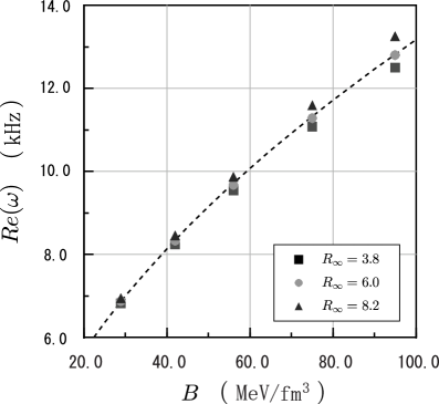
Figure 5: The horizontal axis is the bag constant $B$ (MeV/fm^-3) and the vertical axis is the $f$-mode frequency $Re(\omega)$ . The squares, circles and triangles correspond to the stellar models whose radiation radii are fixed $3.8$, $6.0$ and $8.2$ km, respectively. The dotted line denotes the new empirical formula (22) obtained in Sec. IV between $Re(\omega)$ of $f$-mode and $B$.