Electromagnetic waves around dilatonic stars and naked singularities

Abstract

We study the propagation of classical electromagnetic waves on the simplest four-dimensional spherically symmetric metric with a dilaton background field. Solutions to the relevant equations are obtained perturbatively in a parameter which measures the strength of the dilaton field (hence parameterizes the departure from Schwarzschild geometry). The loss of energy from outgoing modes is estimated as a back-scattering process against the dilaton background, which would affect the luminosity of stars with a dilaton field. The radiation emitted by a freely falling point-like source on such a background is also studied by analytical and numerical methods.

I Introduction

The occurrence of violations of the Equivalence Principle is a subject of continuing investigation in the community of general relativists, both theoretically and experimentally . A possible source for such effects would be the existence of a scalar component of gravity, which naturally emerges in string theories and is usually referred to as the dilaton. Solar system tests rule out such a possibility to a very high precision in the weak field regime will . However, it cannot be excluded that the picture is different in regions of strong gravitational fields, such as those that can be found around very dense compact sources. It is therefore interesting to study solutions of the Einstein field equations with a scalar field.

In this paper, we study the propagation of electro-magnetic (EM) waves on the background of the Janis-Newman-Winicour (JNW) solution jnw . The corresponding metric is spherically symmetric and asymptotically flat, but the static dilaton field is not trivial. Although the JNW space-time is known to contain a naked singularity, it is possible to make it physically useful by suitably cutting the space outside the singular point and then sewing a (spherically symmetric) regular inner patch to complete the space-time manifold. Provided this procedure is carried out consistently, one can then describe compact astrophysical sources such as stars with a dilaton field. In this context, the JNW metric has recently attracted some interest in relation to (strong) gravitational lensing effects bozza .

When the source of EM radiation is placed at the center and is also spherically symmetric, a convenient way of deriving the relevant wave equations is to make use of the Newman-Penrose (NP) formalism chandra . The exact equations thus obtained would however be exceedingly complicated in the full-fledged JNW metric. Therefore, in order to make some progress, we shall introduce a parameter which is related to the asymptotic strength of the dilaton field and can be smoothly perturbed away from the Schwarzschild limit. One then finds that the corresponding wave equations can be solved analytically when the dilaton is sufficiently weak far away from the source and expressions for the ingoing and outgoing modes will be obtained in this approximation. As a straightforward application of this analysis, we shall consider the relative darkening of radiation emitted by a star placed at the center of the system with respect to the vacuum Schwarzschild case. The main result is that such an effect turns out to be inversely proportional to the star radius and to depend on the emitted energy (but not on the wave frequency, contrary to what was found for a rotating black hole knd0 in Ref. knd2 ).

A more complicated problem is to obtain the spectrum of the radiation emitted by a freely falling, electrically charged, point-like source in the JNW background. The wave equations now contain the energy-momentum density of the falling particle and must be solved numerically for various values of the perturbing parameter in order to compare the emitted power to the analogous case in Schwarzschild. A preliminary analytical analysis will show that some effect is already expected at large distance from the center, however most radiation would be emitted near the singularity where tidal forces on the EM field of the falling particle become stronger. Since naked singularities seem to be possible intermediate stages in the gravitational collapse of regular matter (see, e.g. NSreview and References therein), one can view the falling source as a component of the forming collapsed object. Our results may then contribute to the understanding of the (in)stability of naked singularities. The intensity of the radiation shows an interference-like effect which would provide observers with a distinctive signature for the presence of a dilatonic component in strong gravitational fields.

In the following Section, we shall review the JNW solution and express it in terms of the parameter which allows the Schwarzschild limit to be approached in a smooth manner. This property will be used later to define a quasi-Schwarzschild regime, particularly suited for analyzing (asymptotically) small deviations away from Schwarzschild. We then show in Section III how to study electromagnetic waves on such a background using the NP formalism chandra . In Section IV we solve the Maxwell equations using Green function techniques. We finally summarize and comment our results in Section V.

We use units with $G=c=1$ and follow the conventions of Ref. chandra .

II JNW solution and Schwarzschild limit

The JNW metric is a static, spherically symmetric and electrically neutral solution of the field equations obtained by varying the action

$$S = {1\over 16}\,\int d^{4}x\,\sqrt{-g}\,\left[R-{1\over 2}\,\left(\nabla\Phi\right)^{2}\right]$$ (1)

$$-\int d^{4}x\,\sqrt{-g}\,e^{-q\,\Phi}\,F^{2}\ ,$$

in which $R$ is the scalar curvature of the metric $g_{\mu\nu}$, whose determinant is denoted by $g$, $F$ is the EM field strength and note that the dilaton $\Phi$ is included inside the gravitational Lagrangian. Further, the coupling constant $q>0$ between the EM field and the dilaton has also been exponentiated.

For the purpose of studying linear perturbations in the NP formalism chandra , it is convenient to write the JNW metric jnw as

$$ds^{2}={\Delta\over\rho^{2}}\,dt^{2}-{\rho^{2}\over\Delta}\,dr^{2}-\rho^{2}\,d\Omega^{2}\ ,$$ (2)

where $d\Omega^{2}=d\theta^{2}+\sin^{2}\theta\,d\phi^{2}$,

$$\begin{array}[]{l}\rho^{2}=\left(r-r_{-}\right)^{1-a}\,\left(r-r_{+}\right)^{1+a}\\ \\ \Delta=\left(r-r_{-}\right)\,\left(r-r_{+}\right)\ ,\end{array}$$ (6)

and the dilaton field is then

$$\Phi=\sqrt{1-a^{2}}\,\ln\left({r-r_{-}\over r-r_{+}}\right)\ .$$ (7)

Note that, with respect to the original Ref. jnw , $a=1/\mu$ and we have introduced new parameters

$$\begin{array}[]{l}r_{-}=+\displaystyle{r_{0}\over 2}\,{1-a\over a}\\ \\ r_{+}=-\displaystyle{r_{0}\over 2}\,{1+a\over a}\ .\end{array}$$ (11)

Although the JNW metric contains only two independent parameters jnw , the Schwarzschild limit is more conveniently obtained by treating $a$, $r_{-}$ and $r_{+}$ as independent (we just assume $r_{-}<r_{+}$) and separately taking the limits

$$r_{-}\to 0\ \ \ \ {\rm and}\ \ \ a\to-1\ .$$ (12)

The Schwarzschild horizon is then given by $r_{h}\equiv 2\,M=r_{+}$ .

The relevant dilatonic quantity is the spatial derivative

$$\partial_{r}\Phi={\sqrt{1-a^{2}}\,(r_{-}-r_{+})\over(r-r_{-})\,(r-r_{+})}\ ,$$ (13)

which determines the energy-momentum tensor

$$T_{\mu\nu}=\delta^{r}_{\mu}\,\delta^{r}_{\nu}\,\left(\partial_{r}\Phi\right)^{2}-{1\over 2}\,g_{\mu\nu}\,g^{rr}\,\left(\partial_{r}\Phi\right)^{2}\ .$$ (14)

In particular, the non-vanishing components diverge at $r=r_{+}$,

$$T^{t}_{\ t}\sim T^{r}_{\ r}\sim T^{\theta}_{\ \theta}\sim T^{\phi}_{\ \phi}\sim{1-a^{2}\over(r-r_{+})^{2+a}}\ .$$ (15)

and $r_{+}$ is therefore a naked real singularity. Further, since $\rho(r_{+})=0$, such a singularity is point-like and values of $r<r_{+}$ can be considered as unphysical . Let us finally note that the energy-momentum tensor properly vanishes in the limit $a\to\pm 1$ (corresponding to the Schwarzschild vacuum).

The convenient feature of the limit in Eq. (12) is that it is smooth in $r_{-}$ and $a$. This allows us to introduce a quasi-Schwarzschild regime [corresponding to a “small” deviation away from the limit (12)] for the region outside the “horizon” ($0<r_{h}<r$). It is defined by

$$r_{-}=0\ \ \ \ {\rm and}\ \ \ a=-1+2\,x^{2}\ ,$$ (16)

with $0\leq x\ll 1$. In particular, for small $x$, one finds that the metric (2) reduces to Schwarzschild plus corrections of order $x^{2}$,

$$ds^{2} \simeq -\left[1-(1-2\,x^{2})\,{r_{h}\over r}-x^{2}\,{r_{h}^{2}\over r^{2}}\right]\,dt^{2}$$ (17)

$$+\left[1+(1-2\,x^{2})\,{r_{h}\over r}\right]\,dr^{2}+r^{2}\,d\Omega^{2}\ ,$$

where $r_{h}\equiv r_{+}$. The ADM mass for the above metric is given by the usual Schwarzschild relation

$$M={r_{h}\over 2}\ ,$$ (18)

and the relevant PPN parameters will by 

$$\begin{array}[]{l}\alpha=\gamma=1-2\,x^{2}\\ \\ \beta=1-6\,x^{2}\ .\end{array}$$ (22)

In the same approximation, the derivative of the dilaton becomes

$$\partial_{r}\Phi\simeq-{2\,x\over r-r_{h}}\,{r_{h}\over r}\sim-2\,x\,{r_{h}\over r^{2}}\ ,$$ (23)

from which one can see that $x$ is a measure of the dilaton strength for large $r$ (note that $\partial_{r}\Phi$ diverges for $r\to r_{h}$ for all values of $x>0$).

The Eqs. (22) yield a quantitative way of estimating how small the deviations from the Schwarzschild solution are in the weak field zone ($r\gg r_{h}$). From solar test measurements one can therefore read off the bound $x^{2}\lesssim 10^{-5}$ will , which can then be substituted into Eq. (23) to obtain the upper limit of the admissible dilaton strength. Since no direct measurement in the strong field regime is available, the strength of the dilaton field cannot be bounded for $r\sim r_{h}$.

III Dilatonic stars

As we mentioned in the Introduction, the first case we consider is that of a spherically symmetric source for the EM waves placed at the center, so that it can also be identified with the source of the JNW gravitational and dilaton fields. In order to study Maxwell’s equations in this context, we shall take advantage of the spherical symmetry by employing the NP formalism chandra .

III.1 Maxwell waves in NP formalism

We first choose the following contravariant components of the NP tetrad,

$$l^{i}=\left[\begin{array}[]{cccc}{\rho^{2}\over\Delta}\ ,&1\ ,&0\ ,&0\end{array}\right]$$ (25)

$$n^{i}=\left[\begin{array}[]{cccc}{1\over 2}\ ,&-{\Delta\over 2\,\rho^{2}}\ ,&0\ ,&0\end{array}\right]$$ (27)

$$m^{i}=\left[\begin{array}[]{cccc}0\ ,&0\ ,&{1\over\sqrt{2\,\rho^{2}}}\ ,&{i\,{\rm cosec}(\theta)\over\sqrt{2\,\rho^{2}}}\end{array}\right]\ .$$ (29)

The Maxwell field is now completely described by the three complex scalars

$$\phi_{0} \equiv F_{ij}\,l^{i}\,m^{j}$$

$$= {\rho^{3}\over\sqrt{2}\,\Delta}\,\left[E^{\theta}+B^{\varphi}+i\,\sin(\theta)\,\left(E^{\varphi}-B^{\theta}\right)\right]$$

$$\phi_{1} \equiv {1\over 2}\,F_{ij}\,\left(l^{i}\,n^{j}+m^{i*}\,m^{j}\right)$$ (30)

$$= {\rho^{4}\,E^{r}\over 2\,\Delta^{2}}\,\left(1+{\Delta^{2}\over 4\,\rho^{4}}\right)$$

$$\phi_{2} \equiv F_{ij}\,m^{i*}\,n^{j}$$

$$= -{\rho\over 2\,\sqrt{2}}\,\left[E^{\theta}-B^{\varphi}+i\,\sin(\theta)\,\left(E^{\varphi}+B^{\theta}\right)\right]\ ,$$

where $E^{i}$ and $B^{i}$ are the usual electric and magnetic components. The $\phi_{i}$ must satisfy the equations knd

$$(\hat{D}-2\,\tilde{\rho})\,\phi_{1}-(\hat{\delta}^{*}+\tilde{\pi}-2\,\tilde{\alpha})\,\phi_{0}+\tilde{\kappa}\,\phi_{2}=J_{1}$$ (31a)

$$(\hat{\delta}-2\,\tilde{\tau})\,\phi_{1}-(\hat{\Delta}+\tilde{\mu}-2\,\tilde{\gamma})\,\phi_{0}+\tilde{\sigma}\,\phi_{2}=J_{3}$$ (31b)

$$(\hat{D}-\tilde{\rho}+2\,\tilde{\epsilon})\,\phi_{2}-(\hat{\delta}^{*}+2\,\tilde{\pi})\,\phi_{1}+\tilde{\lambda}\,\phi_{0}=J_{4}$$ (31c)

$$(\hat{\delta}-\tilde{\tau}+2\,\tilde{\beta})\,\phi_{2}-(\hat{\Delta}+2\,\tilde{\mu})\,\phi_{1}+\tilde{\nu}\,\phi_{0}=J_{2}\ ,$$ (31d)

with the dilatonic currents

$$J_{1}={q\over 2}\,\left[(\phi_{1}+\phi_{1}^{*})\,\hat{D}-\phi_{0}\,\hat{\delta}^{*}-\phi_{0}^{*}\,\hat{\delta}\right]\Phi$$ (32a)

$$J_{2}={q\over 2}\,\left[(\phi_{1}+\phi_{1}^{*})\,\hat{\Delta}-\phi_{2}\,\hat{\delta}-\phi_{2}^{*}\,\hat{\delta}^{*}\right]\Phi$$ (32b)

$$J_{3}={q\over 2}\,\left[(\phi_{1}-\phi_{1}^{*})\,\hat{\delta}-\phi_{0}\,\hat{\Delta}+\phi_{2}^{*}\,\hat{D}\right]\Phi$$ (32c)

$$J_{4}={q\over 2}\,\left[(\phi_{1}-\phi_{1}^{*})\,\hat{\delta}^{*}+\phi_{0}^{*}\,\hat{\Delta}-\phi_{2}\,\hat{D}\right]\Phi\ .$$ (32d)

In the above, tilded quantities are spin coefficients, and hatted quantities represent differential operators. In particular, the non-vanishing spin coefficients for the JNW metric (2) and tetrad (27) are given by

$$\tilde{\rho} = -\displaystyle{2\,r+r_{+}\,(a-1)-r_{-}\,(a+1)\over 2\,(r-r_{-})\,(r-r_{+})}$$

$$\tilde{\mu} = \displaystyle{2\,r+r_{+}\,(a-1)-r_{-}\,(a+1)\over 4\,(r-r_{-})^{1-a}\,(r-r_{+})^{1+a}}$$

$$\tilde{\alpha} = -\tilde{\beta}$$

$$= -\displaystyle{\sqrt{2}\,{\rm cotan}(\theta)\over 4\,(r-r_{-})^{1-a\over 2}\,(r-r_{+})^{1+a\over 2}}$$

$$\tilde{\gamma} = \displaystyle{a\,(r_{-}-r_{+})\over 4\,(r-r_{-})^{1-a}\,(r-r_{+})^{1+a}}\ .$$

Further, the time dependence of the EM waves is taken to be $\phi_{i}\sim\exp\left(+i\,\omega\,t\right)$, so that the differential operators appearing in the Maxwell equations become

$$\begin{array}[]{l}\hat{D}=\partial_{r}+i\,\displaystyle{\rho^{2}\over\Delta}\,\omega\\ \\ \hat{\Delta}=-\displaystyle{\Delta\over 2\,\rho^{2}}\,\left(\partial_{r}-i\,{\rho^{2}\over\Delta}\,\omega\right)\\ \\ \hat{\delta}=\displaystyle{1\over\sqrt{2\,\rho^{2}}}\,\left[\partial_{\theta}-m\,{\rm cosec}(\theta)\right]\\ \\ \hat{\delta}^{*}=\displaystyle{1\over\sqrt{2\,\rho^{2}}}\,\left[\partial_{\theta}+m\,{\rm cosec}(\theta)\right]\ .\end{array}$$ (41)

Upon substituting the above expressions into Eqs. (31a)-(31d), one obtains the following four equations 

$$\!\!\!\!\!\!\!\left[\partial_{r}+{2\,r+r_{+}\,(a-1)-r_{-}\,(a+1)\over(r-r_{-})\,(r-r_{+})}+i\left({r-r_{+}\over r-r_{-}}\right)^{a}\omega\right]\phi_{1}-{\partial_{\theta}+{\rm cosec}(\theta)\,\left[m+\cos(\theta)\right]\over\sqrt{2}\,(r-r_{-})^{1-a\over 2}\,(r-r_{+})^{1+a\over 2}}\,\phi_{0}$$

$$\ \ \ ={q\over 2}\,\left(\phi_{1}+\phi_{1}^{*}\right)\,\partial_{r}\Phi$$ (42a)

$$\!\!\!\!\!\!\!\left[\partial_{r}+{2\,r-r_{+}\,(a+1)+r_{-}\,(a-1)\over 2\,(r-r_{-})\,(r-r_{+})}-i\left({r-r_{+}\over r-r_{-}}\right)^{a}\omega\right]\phi_{0}+\sqrt{2}\,{\partial_{\theta}-m\,{\rm cosec}(\theta)\over(r-r_{-})^{1+a\over 2}\,(r-r_{+})^{1-a\over 2}}\,\phi_{1}$$

$$\ \ \ ={q\over 2}\,\left[\phi_{0}+2\,\left({r-r_{+}\over r-r_{-}}\right)^{a}\,\phi_{2}^{*}\right]\,\partial_{r}\Phi$$ (42b)

$$\!\!\!\!\!\!\!\left[\partial_{r}+{2\,r+r_{+}\,(a-1)-r_{-}\,(a+1)\over 2\,(r-r_{-})\,(r-r_{+})}+i\left({r-r_{+}\over r-r_{-}}\right)^{a}\omega\right]\phi_{2}-{\partial_{\theta}+m\,{\rm cosec}(\theta)\over\sqrt{2}\,(r-r_{-})^{1-a\over 2}\,(r-r_{+})^{1+a\over 2}}\,\phi_{1}$$

$$\ \ \ =-{q\over 2}\,\left[{\phi_{0}^{*}\over 2}\,\left({r-r_{+}\over r-r_{-}}\right)^{a}+\phi_{2}\right]\partial_{r}\Phi$$ (42c)

$$\!\!\!\!\!\!\!\left[\partial_{r}+{2\,r+r_{+}\,(a-1)-r_{-}\,(a+1)\over(r-r_{-})\,(r-r_{+})}-i\left({r-r_{+}\over r-r_{-}}\right)^{a}\omega\right]\phi_{1}+\sqrt{2}\,{\partial_{\theta}-{\rm cosec}(\theta)\,\left[m-\cos(\theta)\right]\over(r-r_{-})^{1+a\over 2}\,(r-r_{+})^{1-a\over 2}}\,\phi_{2}$$

$$\ \ \ =-{q\over 2}\,\left(\phi_{1}+\phi_{1}^{*}\right)\,\partial_{r}\Phi\ ,$$ (42d)

which we now proceed to study in a suitable limit.

III.2 Quasi-Schwarzschild solutions

We are interested in deviations from Schwarzschild induced by a background dilaton (7) which is experimentally unobservable in the weak field regime. We will therefore look for solutions to Eqs. (42a)-(42d) in the quasi-Schwarzschild regime defined by Eq. (16), bearing in mind that the parameter $x$ is constrained by solar system tests via Eqs. (22) as we mentioned previously.

Upon expanding in $x$, Eq. (42a) becomes

$$\left[\partial_{r}+{2\over r}\left(1+{x^{2}r_{h}\over r-r_{h}}\right)+{i\,\omega\,r\over r-r_{h}}\left(1+2\,x^{2}\ln{r-r_{h}\over r}\right)\right]\phi_{1}-\left(1-x^{2}\,\ln{r-r_{h}\over r}\right){\partial_{\theta}+{\rm cosec}(\theta)\,\left[m+\cos(\theta)\right]\over\sqrt{2}\,r}\,\phi_{0}$$

$$\simeq-q\,x\,{r_{h}\,\sqrt{1-x^{2}}\over r\,(r-r_{h})}\,\left(\phi_{1}+\phi_{1}^{*}\right)\ ,$$ (43)

and analogous expressions are obtained for Eqs. (42b)-(42d). Note that the currents on the right hand sides contain terms proportional to $x$ which are not on the left hand sides. One can then discard all terms of order $x^{2}$ (and higher) and finally obtains

$$\!\!\!\!\!\!\!\!\!\!\!\!\!\!\!\!\!\!\!\!\!\!\!\!\!\!\!\!\!\!\!\!\!\!\!\!\!\!\!\!\!\left(\partial_{r}+{2\over r}+{i\,\omega\,r\over r-r_{h}}\right)\phi_{1}-{\partial_{\theta}+{\rm cosec}(\theta)\,\left[m+\cos(\theta)\right]\over\sqrt{2}\,r}\,\phi_{0}=-q\,x\,{r_{h}\,\left(\phi_{1}+\phi_{1}^{*}\right)\over r\,(r-r_{h})}$$ (44a)

$$\!\!\!\!\!\!\!\!\!\!\!\!\!\!\left(\partial_{r}+{1-i\,\omega\,r\over r-r_{h}}\right)\phi_{0}+\sqrt{2}\,\ln\left(1-{r_{h}\over r}\right)\,{\partial_{\theta}-m\,{\rm cosec}(\theta)\over r-r_{h}}\,\phi_{1}=-{q\,x\,r_{h}\over r-r_{h}}\,\left({\phi_{0}\over r}+{2\,\phi_{2}^{*}\over r-r_{h}}\right)$$ (44b)

$$\!\!\!\!\!\!\!\!\!\!\!\!\!\!\!\!\!\!\!\!\!\!\!\!\!\!\!\!\!\!\!\!\!\!\!\!\!\!\!\!\!\!\!\!\!\!\!\!\!\!\!\!\!\!\!\!\left(\partial_{r}+{1\over r}+{i\,\omega\,r\over r-r_{h}}\right)\phi_{2}-{\partial_{\theta}+m\,{\rm cosec}(\theta)\over\sqrt{2}\,r}\,\phi_{1}=q\,x\,{r_{h}\over r}\,\left({\phi_{0}^{*}\over 2\,r}+{\phi_{2}\over r-r_{h}}\right)$$ (44c)

$$\left(\partial_{r}+{2\over r}-{i\,\omega\,r\over r-r_{h}}\right)\phi_{1}+\sqrt{2}\,\ln\left(1-{r_{h}\over r}\right){\partial_{\theta}-{\rm cosec}(\theta)\,\left[m-\cos(\theta)\right]\over r-r_{h}}\,\phi_{2}=q\,x\,{r_{h}\,\left(\phi_{1}+\phi_{1}^{*}\right)\over r\,(r-r_{h})}\ ,$$ (44d)

where the left hand sides equated to zero are just the wave equations for the EM waves in Schwarzschild.

It is now possible to expand the $\phi_{i}$’s in powers of $x$,

$$\phi_{i}=\phi_{i}^{(0)}+x\,\phi_{i}^{(1)}\ ,$$ (45)

where the $\phi_{i}^{(0)}$’s solve the above Eqs. (44a)-(44d) with vanishing right hand sides. Hence the $\phi_{i}^{(1)}$’s must solve Eqs. (44a)-(44d) with $x=1$.

In the phantom gauge ($\phi_{0}=\phi_{2}=0$ chandra ), $\phi_{1}^{(1)}$ should simultaneously satisfy the four equations

$$\left(\partial_{r}+{2\over r}\pm{i\,\omega\,r\over r-r_{h}}\right)\phi_{1}^{(1)}=\mp q\,{r_{h}\,\left(\phi_{1}^{(1)}+\phi_{1}^{(1)*}\right)\over r\,(r-r_{h})}$$ (46a)

$$\!\!\!\!\!\!\!\!\!\!\!\!\!\!\!\!\!\!\!\!\!\!\!\!\!\!\!\!\!\!\!\!\!\!\!\!\!\!\!\!\!\!\!\!\!\!\!\!\!\!\!\!\!\!\!\!\!\!\!\!\!\left[\partial_{\theta}\pm{m\over\sin(\theta)}\right]\phi_{1}^{(1)}=0\ .$$ (46b)

Eqs. (46b) imply that $$\phi_{1}^{(1)}=\phi_{1}^{(1)}(r)$$. Further, Eqs. (46a) can be written as

$$\begin{array}[]{l}\displaystyle{\left(\partial_{r}+{2\over r}\right)\phi_{1}^{(1)}}=0\\ \\ \ \ i\,\omega\,\phi_{1}^{(1)}=-2\,q\,\displaystyle{r_{h}\over r}\,{\rm Re}\left(\phi_{1}^{(1)}\right)\ ,\end{array}$$ (46f)

and the second condition leads to $\phi_{1}^{(1)}=0$. Since the phantom gauge usually holds for the background solution, this is in agreement with the fact that there is no background EM field in the JNW solution.

For EM waves it is possible to set $\phi_{1}^{(1)}=0$ and define

$$\begin{array}[]{l}W_{0}\equiv\phi_{0}^{(1)}\\ \\ W_{2}\equiv-2\,\phi_{2}^{(1)*}\ ,\end{array}$$ (50)

which must then solve the equations 

$$\!\!\!\!\!\!\!\!\!\!\!\!\!\!\!\!\!\!\!\!\!\!\!\!\!\!\!\!\!\!\!\!\!\!\!\!\!\!\!\!\!\!\!\!\!\!\!\!\!\!\!\!\!\!\left[\partial_{\theta}+{m+\cos(\theta)\over\sin(\theta)}\right]W_{0}=0$$ (51a)

$$\left(\partial_{r}+{1-i\,\omega\,r\over r-r_{h}}\right)W_{0}={q\,r_{h}\over r-r_{h}}\,\left({W_{2}\over r-r_{h}}-{W_{0}\over r}\right)$$ (51b)

$$\left(\partial_{r}+{1\over r}-{i\,\omega\,r\over r-r_{h}}\right)W_{2}={q\,r_{h}\over r}\,\left({W_{2}\over r-r_{h}}-{W_{0}\over r}\right)$$ (51c)

$$\!\!\!\!\!\!\!\!\!\!\!\!\!\!\!\!\!\!\!\!\!\!\!\!\!\!\!\!\!\!\!\!\!\!\!\!\!\!\!\!\!\!\!\!\!\!\!\!\!\!\!\!\!\left[\partial_{\theta}-{m-\cos(\theta)\over\sin(\theta)}\right]W_{2}^{*}=0\ .$$ (51d)

Note that the angular parts of $W_{0}\equiv S_{0}(\theta,\varphi)\,R_{0}(r)$ and $W_{2}\equiv S_{2}(\theta,\varphi)\,R_{2}(r)$ satisfy the independent Eqs. (51a) and (51d). They are thus spherical harmonics with $S_{0}=S_{2}=Y_{l}^{m}(\theta,\varphi)$, the same as for $q=0$. Consequently, the remaining Eqs. (51b) and (51c) become purely radial equations for the $R_{i}(r)$’s,

$$\begin{array}[]{l}R_{0}(r)=e^{i\,\sigma(r)}\,X(r)\\ \\ R_{2}(r)=e^{i\,\sigma(r)}\,Y(r)\ .\end{array}$$ (55)

The real phase $\sigma$ is the same for both fields and satisfies the purely Schwarzschild equation

$${d\sigma\over dr}={\omega\,r\,\sigma\over r-r_{h}}\ .$$ (56)

Hence, $\phi_{0}\sim R_{0}$ represents the ingoing modes while $\phi_{2}\sim R_{2}^{*}$ stands for the outgoing modes. The presence of terms (proportional to $q$) which mix ingoing with outgoing modes immediately implies that outgoing radiation emitted by the central source would partly back-scatter into ingoing waves. Thus the expected dilaton effect is to make the source less bright (see the next Subsection for more quantitative estimates).

The general solutions to the homogeneous equations are given by

$$\begin{array}[]{l}\phi_{0}^{(0)}=A\,\displaystyle{e^{+i\,\sigma(r)}\over r-r_{h}}\,Y_{l}^{m}(\theta,\varphi)\\ \\ \phi_{2}^{(0)}=B\,\displaystyle{e^{-i\,\sigma(r)}\over r}\,Y_{l}^{-m}(\theta,\varphi)\ ,\end{array}$$ (60)

where $\sigma$ solves Eq. (56) and the constants $A$ and $B$ must be determined from the initial conditions.

The functions $X$ and $Y$ must solve

$$\left(\partial_{r}+{1\over r-r_{h}}\right)X={q\,r_{h}\over r-r_{h}}\,\left({Y\over r-r_{h}}-{X\over r}\right)$$ (61a)

$$\!\!\!\!\!\!\!\!\!\!\!\!\!\!\!\left(\partial_{r}+{1\over r}\right)Y={q\,r_{h}\over r}\,\left({Y\over r-r_{h}}-{X\over r}\right)\ .$$ (61b)

Since $E^{2}\sim B^{2}\sim 1/r^{2}$ for large $r$, admissible solutions to Eqs. (61a) and (61b) should be of order $1/r$ or higher at large $r$, as occurs to the $\phi_{i}^{(0)}$’s. In fact, the particular solutions are given by

$$\begin{array}[]{l}X=\displaystyle{C\over r-r_{h}}\,\left[q\,\ln\left(1-{r_{h}\over r}\right)-1\right]\\ \\ Y=q\,\displaystyle{C\over r}\,\ln\left(1-{r_{h}\over r}\right)\ ,\end{array}$$ (65)

where $C$ is a constant. Note also that the limit $q\to 0$ yields a solution of the homogeneous (purely Schwarzschild) equations ($\phi_{0}^{(1)}=\phi_{0}^{(0)}$ and $\phi_{2}^{(1)}=0$).

The exchange of energy between ingoing and outgoing waves becomes more apparent by adding the homogeneous parts (60) and reshuffling the constants $A$, $B$ and $C$ so as to write the general solution as

$$\!\!\!\!\!\!\begin{array}[]{l}\phi_{0}=A\,\displaystyle{e^{+i\,\sigma}\over r-r_{h}}\,\left[1+\tilde{x}\,{B-A\over A}\,\ln\left(1-{r_{h}\over r}\right)\right]Y_{l}^{m}\\ \\ \phi_{2}=B\,\displaystyle{e^{-i\,\sigma}\over r}\,\left[1+\tilde{x}\,{B-A\over B}\,\ln\left(1-{r_{h}\over r}\right)\right]Y_{l}^{-m}\ ,\end{array}$$ (69)

where $\tilde{x}\equiv q\,x>0$ is an effective coupling constant between the EM field and the dilaton, and the constants $A=A_{lm}(\omega)$ and $B=B_{lm}(\omega)$ must be determined from the initial conditions. There is obviously no initial condition (choice of $A$ and $B$) which can produce just ingoing ($\phi_{0}$) or just outgoing ($\phi_{2}$) waves.

III.3 Darkened stars

Let us denote by $r_{e}>r_{h}$ the outer radius of the central star and consider the case $A=0$, corresponding to a purely outgoing mode $\phi_{2}$ in Schwarschild ($\tilde{x}=0$). The ratio between the energy of such an EM wave ($\sim\phi_{2}^{2}$) at the point of emission $r=r_{e}$ and at the point of observation $r=r_{o}$ would be

$$\Gamma_{\rm Schw}\simeq\left[{\phi_{2}^{(0)}(r_{e})\over\phi_{2}^{(0)}(r_{o})}\right]^{2}\sim\left({r_{o}\over r_{e}}\right)^{2}\ .$$ (70)

The same quantity in JNW (evaluated to leading order in $\tilde{x}$) is obtained from the solution in Eq. (69),

$$\Gamma_{\rm JNW}\sim\left({r_{e}\over r_{o}}\right)^{2}\,{1+2\,\tilde{x}\,(1-{1/B})\,\ln\left(1-{r_{h}\over r_{e}}\right)\over 1+2\,\tilde{x}\,(1-{1/B})\,\ln\left(1-{r_{h}\over r_{o}}\right)}\ ,$$ (71)

where $B$ can be determined, e.g. from the energy $E_{o}$ at the point of observation,

$$B^{2}\sim r_{o}^{2}\,E_{o}\ .$$ (72)

On assuming that $r_{h}\ll r_{e}\ll r_{o}$ (a safe assumption to protect the star from the central singularity), one finds

$$\Gamma_{\rm JNW}\sim\Gamma_{\rm Schw}\,\left[1-2\,\tilde{x}\,\left(1-{1\over r_{o}\,\sqrt{E_{o}}}\right)\,{r_{h}\over r_{e}}\right]\ ,$$ (73)

which shows a peculiar dependence on the energy of the wave. This dependence is not seen in the Schwarzschild case. In particular, since $\tilde{x}>0$ and the term in round brackets is positive for realistic cases, the flux is weaker than in the Schwarzschild vacuum.

With respect to what was found for the Kerr-Newman-dilaton black hole knd2 , let us note that the final result does not show a frequency dependence. This can be understood since the static case we are now considering has no typical frequency, whereas the rotating case has intrinsic angular velocity.

IV Freely falling source

A possible source of electromagnetic radiation from a dilatonic black hole is the radiation emitted by a charged particle falling freely into the black hole. In fact, the curved background distorts the EM field of the falling charge and causes the latter to release energy as though it were being accelerated in a Lorentz frame.

For practical purposes, it is more convenient to regard the falling charge $Q$ as distorting the background EM field $F_{\mu\nu}^{(0)}$ of the black hole, and expand the exact $F_{\mu\nu}$ to linear order in $Q$ as

$$F_{\mu\nu}=F_{\mu\nu}^{(0)}+Q\,F_{\mu\nu}^{(1)}\ .$$ (74)

Since in our case $F_{\mu\nu}^{(0)}=0$, the perturbed EM tensor elements $F_{\mu\nu}^{(1)}$ are determined by the Maxwell-dilaton equation

$$\partial_{\nu}\left(\sqrt{-g}\,e^{-q\,\Phi}\,F^{(1)\,\mu\nu}\right)=4\,\pi\,\sqrt{-g}\,j^{\mu}\ ,$$ (75)

where $Q\,j^{\mu}$ is the current associated with the falling charge. The metric tensor elements are given in Eq. (2) and, in order to solve the set of Eqs. (75), the (antisymmetric) perturbations $F_{\mu\nu}^{(1)}$ are conveniently expanded in tensor harmonics zerilli

$$F_{\mu\nu}^{(1)}=\left[{\begin{array}[]{cccc}0&f_{01}\,Y_{l}^{m}&f_{02}\,\partial_{\theta}Y_{l}^{m}&-f_{02}\,\sin(\theta)\,\partial_{\phi}Y_{l}^{m}\\[8.61108pt] *&0&f_{12}\,\partial_{\theta}Y_{l}^{m}&f_{12}\,\partial_{\phi}Y_{l}^{m}\\[8.61108pt] *&*&0&0\\[8.61108pt] *&*&0&0\end{array}}\right]\ ,$$ (80)

where the $f_{ij}$’s depend only on $r$ and $t$ (and carry integer indices $l$ and $m$ which we omit), the $Y_{l}^{m}$’s are again the normalized spherical harmonics, and the asterisks ($*$) denote the negative of the corresponding transposed tensor element. The field tensor given in Eq. (80) is for electric multipoles. Further, using the field equations all of the tensor elements $F_{\mu\nu}^{(1)}$ can be put in terms of a single element, say $f_{12}$.

The function $f_{12}$ is assumed to be of the form

$$f_{12}(r,t)=\hat{f}_{12}(r)\,\exp(i\,\omega\,t)\ .$$ (81)

Upon substitution of this expression into the equation for $f_{12}$ and expanding to first order in $\tilde{x}\equiv q\,x$, the function $\hat{f}_{12}$ satisfies the equation

$${d^{2}\hat{f}_{12}\over{dr^{2}}}+{r_{h}\,(3+2\,\tilde{x})\over{r\,(r-r_{h})}}\,{d\hat{f}_{12}\over{dr}}+\left[{\omega^{2}\,r^{2}\over(r-r_{h})^{2}}-{r_{h}\,(2\,r-3\,r_{h})\over{r^{2}\,(r-r_{h})^{2}}}\,(1+2\,\tilde{x})-{l\,(l+1)\,\over{r\,(r-r_{h})}}\right]\,\hat{f}_{12}=S(r)\ ,$$ (82a)

where the source term is given by

$$S(r)=-{e^{i\,\omega\,T(r)}\over(r-r_{h})^{2}}\,\left[1-2\,\tilde{x}\,\ln\left(1-{r_{h}\over r}\right)\right]\ ,$$ (82b)

and

$$T(r)=r_{h}\left[2\,{r^{1/2}\over r_{h}^{1/2}}-{2\,r^{3/2}\over 3\,r_{h}^{3/2}}+\ln{(r/r_{h})^{1/2}-1\over(r/r_{h})^{1/2}+1}\right]$$ (82c)

is the time (to order $\tilde{x}^{2}$) for the particle to fall from $\infty$ to the point $r$.

IV.1 Green’s function method

Eq. (82a) is a typical Sturm-Liouville problem which can be solved with the aid of the Green’s function $G(r,r^{\prime})$. The latter is defined, for $r\not=r^{\prime}$, as a solution of the homogenous equation obtained from Eq. (82a) by setting $S(r)=0$ and, for $r=r^{\prime}$, by the boundary condition $G(r,r)=1$. In terms of $G$ the solution of Eq. (82a) is then given by

$$\hat{f}_{12}(r)=\int G(r,r^{\prime})\,S(r^{\prime})\,dr^{\prime}\ ,$$ (83)

where $S(r)$ is the source term (82b)

The homogenous equation which determines $G$ is of the form

$$A_{2}\,G^{\prime\prime}+A_{1}\,G^{\prime}+A_{0}\,G=0\ ,$$ (84)

where the coefficients $A_{i}$ are determined by comparison with Eq. (82a) and a prime denotes the partial derivative with respect to the first argument of $G=G(r,r^{\prime})$.

Before attempting to solve Eq. (84) numerically, it is interesting to estimate analytically the effect of the dilaton at large distance from the singularity. We fist expand the coefficients $A_{i}$’s in powers of $1/r$ and keep only next-to-leading terms. Then we expand the Green’s function in powers of $\tilde{x}$ and write $G=G_{0}+\tilde{x}\,G_{1}$. To order $\tilde{x}^{0}$, Eq. (84) then yields

$$\hat{L}\,G_{0} \equiv \left(1+3{r_{h}\over r}\right)G_{0}^{\prime\prime}-3{r_{h}\over r^{2}}\,G_{0}^{\prime}+\omega^{2}\left(1+{5\,r_{h}\over 3\,r}\right)G_{0}$$ (85a)

$$= 0$$

and, to order $$\tilde{x}^{1}$$,

$$\hat{L}\,G_{1}=\omega^{2}\,{5\,r_{h}\over 3\,r}\,G_{0}\equiv S_{G}\ .$$ (85b)

One thus finds that $G_{1}$ satisfies the same equation as $G_{0}$ plus a source term determined by $G_{0}$ which does not vanish too rapidly at large $r$. One can therefore expect significant corrections with respect to the Schwarzschild case ($\tilde{x}=0$) at relatively large distances from the central singularity.

It is not necessary to solve Eq. (85b) explicitly. One can instead include the right hand side of Eq. (85b) in the source $S$ and write the solution to Eq. (82a) simply in terms of $G_{0}$ as

$$\hat{f}_{12}(r) = \int G_{0}(r,r^{\prime})\,S_{0}(r^{\prime})\,dr^{\prime}+\tilde{x}\int G_{0}(r,r^{\prime})\,S_{1}(r^{\prime})\,dr^{\prime}$$ (86)

$$+\tilde{x}\,\int G_{1}(r,r^{\prime})\,\left[S_{0}(r^{\prime})+S_{G}(r^{\prime})\right]\,dr^{\prime}$$

$$= (1+\tilde{x})\int G_{0}(r,r^{\prime})\,S_{0}(r^{\prime})\,dr^{\prime}$$

$$+\tilde{x}\int G_{0}(r,r^{\prime})\,\left[S_{1}(r^{\prime})+S_{G}(r^{\prime})\right]\,dr^{\prime}\ ,$$

in which we also expanded $S=S_{0}+\tilde{x}\,S_{1}$ and retained terms to order $\tilde{x}^{1}$.

Unfortunately Eq. (85a) is already rather complicated, and the terms of higher order in $1/r$ which we dropped make the problem intractable analytically. Hence, we proceed now to solve Eq. (82a) numerically and discuss the energy distribution.

IV.2 Numerical results

Once the function $\hat{f}_{12}$ has been determined, the energy distribution corresponding to the angular mode $l$ and averaged over the complete solid angle is given by

$$\mbox{$\left\langle\,\displaystyle{\frac{dE}{d\omega}}\,\right\rangle$}={\frac{l\,(l+1)}{2\,\pi}}\,\hat{f}_{12}^{\ }\,\hat{f}^{*}_{12}\ .$$ (87)

The energy distribution (87) is plotted as a solid line in Fig. 1 for unit charge $Q$ and black hole mass $M$ ($=r_{h}/2$) and with the angular mode $l=1$. The energy of the radiation is

$$\Delta E\simeq C_{(4)}\,\frac{Q^{2}}{M}\ ,$$ (88)

where $C_{(4)}$ is the area under the curve. The secondary peak at higher frequencies in this distribution distinguishes the dilatonic black hole from the Schwarzschild black hole, which has only one peak (see the $2^{\rm nd}$ Reference of zerilli ). This suggests an interference between the dilatonic and tensor contributions to the electromagnetic field components. The secondary peak has an amplitude which is an appreciable fraction of the higher peak at $\omega\approx 2.7$. Such a peak should be relatively easy to detect. The observation of such an interference term would be evidence for the existence of a scalar component of gravity.

${1\over Q^{2}}\,{dE\over d\omega}$
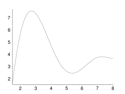
                                                    ${\omega\,r_{h}}$

Figure 1: Energy distribution for a particle of unit charge falling into a four-dimensional black hole of mass $M$.

V Conclusions

We have analyzed the propagation of EM waves in the background of the Janis-Newman-Winicour (JNW) solution. To obtain manageable expressions describing the relevant physical quantities, e.g. the energy of the emitted waves and the intensity as a function of frequency, we have had to expand the metric tensor elements in terms of a small parameter $\tilde{x}$ which measures the deviation of the JNW solution from the Schwarzschild solution at large distance from the singularity. This is a reasonable thing to do because the effect of a scalar component of gravity on the aforementioned quantities is most likely small. We have applied the resulting expansions to two cases of physical interest.

The first case is that of a star with a dilatonic field. We have obtained approximate analytic expressions for the ingoing and outgoing wave functions in terms of the small expansion parameter, $\tilde{x}$. From these expressions we can calculate the luminosity of the object emitting the radiation and we find that its luminosity is reduced by the dilaton background. Such a reduction would affect the luminosity-to-distance relations that are used to determine the distance of astrophysical objects.

In the second case we have described the emission from a point-like charged particle freely falling in the chosen background. In this case the JNW metric is expanded in terms of the small parameter $\tilde{x}$ in order to obtain a simple form for the second order differential equation whose solution is (the Fourier transform of) the wave amplitude. We have checked that setting the parameter $\tilde{x}$ to zero gives the same differential equation as was obtained in zerilli for the Schwarzschild case. For nonzero $\tilde{x}$ the frequency distribution curve $dE/d\omega$ differs significantly from that obtained for the Schwarzschild metric. Models of the radiation from compact astrophysical sources incorporating this effect would provide a test of the existence of a scalar component of gravity.

References

• (1) C.M. Will, Theory and experiment in gravitational physics, 2nd ed., Cambridge University Press 1993; Living Rev. Rel. 4 (2001) 4.
• (2) A.I. Janis, E.T. Newman and J. Winicour, Phys. Rev. Lett. 20 (1968) 878.
• (3) V. Bozza, Phys. Rev. D 66 (2002) 103001.
• (4) S. Chandrasekhar, The Mathematical Theory of Black Holes (Oxford University Press, Oxford, 1983).
• (5) R. Casadio, B. Harms, Y. Leblanc and P.H. Cox, Phys. Rev. D 55, 814 (1997).
• (6) R. Casadio and B. Harms, Phys. Rev. D 60, 104017 (1999).
• (7) T. Harada, H. Iguchi and K. Nakao, Prog. Theor. Phys. 107, 449 (2002).
• (8) F. Finelli and A. Gruppuso, in preparation.
• (9) R. Casadio, B. Harms, Y. Leblanc and P.H. Cox, Phys. Rev. D 56, 4948 (1997).
• (10) F. Zerilli, Phys. Rev. D 9, 860 (1974); M. Johnston, R. Ruffini, F. Zerilli, Phys. Lett. B49, 185 (1974).