The asymptotic quasinormal mode spectrum of non-rotating black holes

Abstract

A conjectured connection to quantum gravity has led to a renewed interest in highly damped black hole quasinormal modes (QNMs). In this paper we present simple derivations (based on the WKB approximation) of conditions that determine the asymptotic QNMs for both Schwarzschild and Reissner-Nordström black holes. This confirms recent results obtained by Motl and Neitzke, but our analysis fills several gaps left by their discussion. We study the Reissner-Nordström results in some detail, and show that, in contrast to the asymptotic QNMs of a Schwarzschild black hole, the Reissner-Nordström QNMs are typically not periodic in the imaginary part of the frequency. This leads to the charged black hole having peculiar properties which complicate an interpretation of the results.

I Background and motivation

I.1 The quasinormal modes

Black holes oscillate. The associated quasinormal modes (QNMs) of oscillation are relevant for many reasons. Most importantly, numerical relativity has provided ample evidence that the QNMs dominate the gravitational-wave signal associated with many processes involving dynamical black holes (such as the formation of black holes in gravitational collapse or binary merger). Since the QNMs encode information concerning the parameters of the black hole one may hope that the gravitational-wave detectors that are now coming into operation will be able to use these signals to investigate the black hole population of the Universe.

Even though most studies of QNMs have been motivated by their potential astrophysical relevance, there are several other reasons why one might be interested in understanding the spectrum of oscillations of a black hole. In particular, the modes have played a key role in discussions of black hole stability whiting . A closely related issue concerns mode-completeness. It now seems clear that the QNMs do not form a complete set (at least not in the conventional sense) because of the presence of power-law tails caused by the backscattering of waves (see naprd for a discussion and references). The problem also has interesting computational aspects. While the slowly damped QNMs, for which $|\mbox{Re }\omega M|>>|\mbox{Im }\omega M|$, are relatively easy to compute, highly damped modes present a challenge. The main difficulty concerns the fact that, in the frequency domain, the QNM eigenfunctions (which represent purely outgoing waves at spatial infinity and purely ingoing waves crossing the event horizon) grow exponentially. This means that one must, in principle, achieve exponential precision in order to impose the boundary conditions. The first reliable calculation of high QNM overtones was performed by Leaver in the mid-1980s using continued fractions leaver1 . An alternative approach to the problem proceeds via analytic continuation using complex coordinates, borrowing standard asymptotic techniques from quantum mechanics. In particular, this was the fundamental idea behind the numerical phase-amplitude method that has been used to calculate high precision QNMs of both Schwarzschild and Reissner-Nordström black holes pam1 ; pam2 . Both these results, and those of Nollert and Schmidt ns , agreed with those of Leaver.

While the reliability of Leaver’s method is now well established, it was not without controversy a decade ago. The discussion concerned the behaviour of the QNMs in the limit of very high damping. Leaver’s results (for the first fifty modes of a Schwarzschild black hole) indicated that the modes would asymptotically behave as

$$\omega_{n}M\sim 0.08-{i\over 4}(2n+1)\quad\mbox{ as }n\to\infty$$

This was contradicted by results obtained by Guinn et al using a WKB formula guinn . Their calculation suggested that the real part of the QNM frequencies would vanish asymptotically. The controversy was resolved by two calculations which agreed that the correct asymptotic result was

$$\omega M\sim 0.04371235-{i\over 4}(2n+1)\quad\mbox{ as }n\to\infty$$ (1)

The first calculation was based on a slight reformulation of the continued fraction algorithm noll , while the second used a high order phase-integral formula al ; nacqg . The latter calculation also shed light on the reasons for the breakdown of the method used by Guinn et al. guinn . This issue is further discussed in Refs. pimrev ; gbs .

I.2 Is there a quantum connection?

Despite the fact that the laws of black-hole thermodynamics are by now well established, many issues remain unclear. It is, for example, not clear to what extent the black hole entropy

$$S={A\over 4}$$ (2)

where $A$ is the area of the event horizon, can be understood in terms of the statistics of a given set of microstates. (We use units such that $c=G=\hbar=1$ throughout the paper.) Bekenstein and colleagues have discussed this problem in terms of a quantised area (see for example bmuk ). Then, in analogy with a typical finite system, a black hole would have a discrete spectrum. One can argue that bmuk

$$A=n4\ln k\qquad\mbox{ with }n=1,2,3,...\mbox{ and }k=2,3,4,...$$ (3)

Comparing this with

$$A=16\pi M^{2}\rightarrow\Delta A=32\pi M\Delta M=32\pi M\omega$$ (4)

where we have associated the “energy spacing” with a frequency through $\Delta M=\Delta E=\omega$ (roughly speaking, $\omega$ corresponds to a “transition energy”), one finds that the spacing between consecutive states (for macroscopic black holes, with $M>>\hbar$) will correspond to a frequency

$$\omega={\ln k\over 8\pi M}$$ (5)

The standard argument, which favours $k=2$, would make the entropy spacing between energy levels exactly one “bit”, which is attractive from the information theory point of view. A key result is that, in this picture any radiation will be emitted in multiples of the fundamental frequency $\omega$. Hence, essentially no radiation should be radiated with frequencies below $\omega$. If true, this is a highly significant conclusion since it suggests that the quantum nature of black holes might be observable at the macroscopic level.

As has been demonstrated by Ashtekar and his collaborators ash1 , one can arrive at the same conclusions within the framework of loop quantum gravity (see ash2 for a nice introduction). This approach is based on the notion of quantum geometry, which means that it is natural to ask what the quantum of area might be. Again, it is possible to draw conclusions from considerations of macroscopic black holes. For large black holes it has been shown that ash1

$$A=n\gamma_{BI}4\pi\sqrt{3}$$ (6)

The parameter $\gamma_{BI}$ is an unknown “natural constant” called the Barbero-Immirzi parameter. It plays an important role because it fixes an ambiguity in the theory. If this parameter could be determined by an independent “experiment” the theory would become predictive. In fact, the Barbero-Immirzi parameter can be fixed by carrying out a calculation of the black-hole entropy and comparing to the standard result, Eq. (2). By attributing entropy to microstates (actually nodes of spin networks, see ash2 ) it can be shown that

$$S={\ln 2\over 4\pi\sqrt{3}\gamma_{BI}}A\rightarrow\gamma_{BI}={\ln 2\over\pi\sqrt{3}}$$ (7)

provided that the lowest permissible spin is $1/2$. Again the area quantum is $\Delta A=4\ln 2$.

So what does this have to do with the black hole QNMs? The possible connection between the classical vibrations of a black-hole spacetime and various quantum aspects has been discussed for quite some time. For an early contribution to the debate, see Ref. york . The recent interest in a possible association between the two problems followed a very simple observation. A few years ago, Hod hod noticed that the numerical results for asymptotic Schwarzschild QNMs seemed to suggest that

$$\mbox{Re }\omega M\to{\ln 3\over 8\pi}\quad\mbox{ as }|\mbox{Im }\omega|\to\infty$$ (8)

If we identify the (real part of the) asymptotic QNM frequency with the quantum interstate spacing, we can use this value in (4) to get

$$\omega={\ln 3\over 8\pi M}\rightarrow\Delta A=4\ln 3$$ (9)

This is a tantalizing result. It would fit nicely into Bekenstein’s thermodynamical picture provided that the “fundamental” frequency is associated with $k=3$ rather than 2. Furthermore, Dreyer dreyer has shown that this would be the prediction of loop quantum gravity if it were based on SO(3) rather than SU(2). In this case the predicted Barbero-Immirzi parameter would be

$$\gamma_{BI}={\ln 3\over 2\pi\sqrt{2}}$$ (10)

There are, of course, problems associated with this change. In particular, SO(3) is not favoured because it would seem not to allow coupling to fermions. Hence, one would need to either explain why fermions should be excluded cor , or provide an alternative derivation of the black hole entropy (perhaps using a different statistics for the quantised area states poly ). Various other relevant issues have been discussed in Refs. kun ; kaul ; birm .

On the other hand, we now have a testable prediction. If Hod’s argument holds, one should be able to learn something useful from, for example, the asymptotic behaviour of the Reissner-Nordström QNM frequencies. However, until very recently only the slowly damped QNMs of Reissner-Nordström black holes had been calculated gunt ; kokk ; pam2 ; leaver2 ; aas .

The present paper is motivated by the recent discussion motl ; motl2 ; mvdb ; bk ; neitzke . Our aim is to use the complex coordinate WKB method heading ; fandf ; bam in its very simplest form to determine asymptotic QNMs for Schwarzschild and Reissner-Nordström black holes. As we will see, this leads to results that agree with those of Motl and Neitzke motl2 . Furthermore, our analysis fills several gaps left by their study and extends the discussion of the final result considerably.

II Key principles of the complex coordinate WKB analysis

The equations governing various classes of non-rotating black-hole perturbations can be written chandra

$${d^{2}\psi\over dr_{\ast}^{2}}+[\omega^{2}-V(r)]\psi=0$$ (11)

where we have assumed that the perturbations depend of time as $e^{-i\omega t}$. The tortoise coordinate is defined by

$${dr_{\ast}\over dr}={r^{2}\over\Delta}$$ (12)

where $\Delta$ depends on the spacetime geometry, and is here given by

$$\Delta=r^{2}-2Mr+q^{2}$$ (13)

where $M$ is the mass of the black hole and $q$ is its electric charge. The two solutions to $\Delta=0$ determine the location of the event horizon $r_{+}=M+\sqrt{M^{2}-q^{2}}$ and, for charged black holes, the inner Cauchy horizon $r_{-}=M-\sqrt{M^{2}-q^{2}}$. The definition (12) is such that the causally attainable spacetime region outside the black hole, $r_{+}<r<\infty$, is mapped onto $-\infty<r_{\ast}<\infty$. The effective potential $V(r)$ is of short range, which means that $\psi\sim e^{\pm i\omega r_{\ast}}$ both near the horizon and at infinity. With our chosen time-dependence the solution behaving as $e^{i\omega r_{\ast}}$ represents an outgoing wave at infinity, while $e^{-i\omega r_{\ast}}$ is a ingoing wave near the horizon.

It is easy to explain one of the main difficulties associated with the QNM problem. Suppose we want to calculate a damped QNM, i.e. a solution for which Im $\omega M<0$. Then the solution that represents outgoing waves at infinity will grow exponentially as $r_{\ast}$ increases. This means that we will need exponential precision in order to filter out the ingoing-wave contribution and impose the desired boundary condition. This is not a straightforward computational task. A similar difficulty arises with the boundary condition at the horizon. However, the problem becomes straightforward if we analytically continue into the complex coordinate plane. Suppose, for example, that we analyse the problem along a line such that $\omega r_{\ast}$ is purely real. Then the two asymptotic solutions would be purely oscillatory and it would be easy to impose the boundary conditions. Of course, before we can benefit from this idea we must understand how the solutions change under analytic continuation. Fortunately, the relevant principles are well known from WKB/phase-integral theory. In fact, in this paper we will only use results that were well understood at least 40 years ago heading ; fandf ; bam . The advantage of this kind of analysis is that it does not require the use of complicated comparison equations to spot special solutions whose analytic properties can be exploited (it is an “atomic” description rather than a “molecular” one).

In order to analyse the black hole problem we prefer to work in the complex $r$-plane (this is natural since the tortoise coordinate is multi-valued). Introducing a new dependent variable

$$\Psi=\left({\Delta\over r^{2}}\right)^{1/2}\psi$$ (14)

we readily rewrite the perturbation equation as

$${d^{2}\Psi\over dr^{2}}+R(r)\Psi=0$$ (15)

where

$$R(r)=\left({r^{2}\over\Delta}\right)^{2}\left\{\omega^{2}-V(r)+{1\over 4}\left[{d\over dr}\left({\Delta\over r^{2}}\right)\right]^{2}-{1\over 2}{\Delta\over r^{2}}{d^{2}\over dr^{2}}\left({\Delta\over r^{2}}\right)\right\}$$ (16)

As is well known, the two WKB solutions to an equation of form (15) can be written

$$f_{1,2}^{(t)}(r)=Q^{-1/2}(r)\exp\left[\pm i\int_{t}^{r}Q(r^{\prime})dr^{\prime}\right]$$ (17)

with $Q^{2}=R$. However, under some circumstances it is useful to use a slightly different function as basis for the approximation. As we will discuss in the next section, we will exercise this freedom in our analysis of the asymptotic black hole problem. Note that, without loss of generality, the lower limit of integration $t$ is customarily taken to be one of the zeros of $Q$. Throughout this paper we will indicate the relevant lower limit of integration by a subscript on $f_{1,2}$ as in (17).

The zeros and poles of the function $Q$ play a central role in any complex coordinate analysis of (15). From each simple zero of $Q^{2}$ emanates three so-called “Stokes lines”. Along each of these contours $Q(r)dr$ is purely imaginary, which means that one of the two solutions grows exponentially, while the second solution decays, as we move away from $t$. In other words, one of the solutions is exponentially dominant on the Stokes line, while the other solution is sub-dominant. Analogously, one can define three “anti-Stokes lines” associated with each simple zero of $Q^{2}$. On anti-Stokes lines $Q(r)dr$ is purely real, which means that the two solutions are purely oscillatory. As we cross an anti-Stokes line, the dominancy of the two functions $f_{1,2}$ changes. The three-fold symmetry associated with each zero of $Q^{2}$ is clear from Figs. 1 and 2.

Stokes lines are vital for WKB analysis, because it is in the vicinity of these contours that the solution changes character. That is, if the solution is appropriately represented by a certain linear combination of $f_{1}$ and $f_{2}$ in some region of the complex $r$-plane, the linear combination will change as the solution is extended across a Stokes line. The induced change is not complicated: The coefficient of the dominant solution remains unchanged, while the coefficient of the solution which is subdominant on the relevant Stokes line picks up a contribution proportional to the coefficient of the dominant solution. This is known as the “Stokes phenomenon” stokes . The contant of proportionality is known as a “Stokes constant”. This change is necessary for the particular representation (17) to preserve the monodromy of the global solution. Terms that are exponentially small in one sector of the complex plane may be overlooked. However, in other sectors they can grow to exponentially dominate the solution. By incorporating the Stokes phenomenon, we have a formally exact procedure which leads to a proper account of all exponentially small terms.

In the particular case of an isolated simple zero $t$ of $Q^{2}$ the problem is straightforward heading ; fandf . Suppose that the solution in the initial region of the complex plane is given by

$$\Psi=cf_{1}^{(t)}$$ (18)

Then, after crossing a Stokes line emanating from $t$ (and on which $f_{1}$ is dominant) the solution becomes

$$\Psi=cf_{1}^{(t)}\pm icf_{2}^{(t)}$$ (19)

The sign depends on whether one crosses the Stokes line in the positive (anti-clockwise) or negative (clockwise) direction. It is crucial to note that this simple result, i.e. that the Stokes constant is $\pm i$, only holds when the Stokes line emanates from the zero that is used as lower limit for the phase-integral. That is, when we want to use the above result to construct an approximate solution valid in various regions of the complex plane we must often change the reference point for the phase-integral. This leads to the need to evaluate integrals of the type

$$\gamma_{ij}=\int_{t_{i}}^{t_{j}}Q(r)dr$$ (20)

where ${t_{i}}$ and ${t_{j}}$ are two simple zeros of $Q^{2}$.

A final issue that must be mentioned before we proceed concerns branch cuts. In general we need to introduce branch cuts from the simple zeros of $Q^{2}$ in order to ensure that the phase integrands remain single-valued. However, one can usually place these cuts in such a way that they do not affect the analysis. In the following derivations this is the case. We will choose the phase of the square-root of $Q^{2}$ such that

$$Q=R^{1/2}\sim\omega\quad\mbox{ as }r\to\infty$$ (21)

This means that the outgoing-wave solution at infinity is proportional to $f_{1}$ while the ingoing-wave solution at the horizon is proportional to $f_{2}$.

III The Schwarzschild problem

III.1 Evaluating the phase-integrals

In the case of Schwarzschild black holes (when $q=0$) there are two classes of gravitational perturbations, usually refered to as axial and polar chandra . We will only consider the axial case here. This is, however, no restriction since it has been shown that the two cases are isospectral chandra . That is, the QNMs are the same in both cases. Once we have derived the relevant WKB condition for axial gravitational perturbations we will discuss the case of electromagnetic waves in the Schwarzschild background.

In the case of axial gravitational perturbations, the effective potential is

$$V={\Delta\over r^{2}}\left[{(l(l+1)\over r^{2}}-{6M\over r^{3}}\right]\qquad l=2,3,4,...$$ (22)

From this and Eq. (16) we deduce that the function $R$ has two second order poles and four zeros. Since the zeros are closely associated with the Stokes phenomenon, we need to know their location, as well as the nature of the Stokes and anti-Stokes lines. It is easy to show that, when Im $\omega\to-\infty$ the zeros all approach the origin of the complex $r$-plane. This allows us to simplify the analysis considerably. Expanding in a power series near $r=0$ we have

$$R\approx{r^{2}\over 4M^{2}}\left[\omega^{2}-{15M^{2}\over r^{4}}\right]\approx-{15\over 4r^{2}}$$ (23)

sufficiently near to the origin. Note that this approximation contains no reference to $l$. As $|\omega|\to\infty$ the $l$-dependent terms are only higher order corrections.

Given this behaviour it is easy to show that the exact solutions to (15) should behave like

$$\Psi\sim r^{1/2\pm 2}\quad\mbox{ as }r\to 0$$ (24)

Meanwhile, if we take $Q^{2}=R$ we get

$$Q^{-1/2} \sim r^{-1/2}$$ (25)

$$\int Qdr \sim \pm i\sqrt{15\over 4}\ln r$$ (26)

which means that

$$f_{1,2}\sim r^{1/2\pm\sqrt{15/4}}$$ (27)

In other words, the approximate solutions do not have the correct behaviour in the vicinity of the origin. However, by choosing

$$Q^{2}=R-{1\over 4r^{2}}$$ (28)

we obtain approximate solutions with the desired behaviour near the origin. This is analogous to the “Langer modification” $l(l+1)\to(l+1/2)^{2}$ that is used in the WKB analysis of radial quantum problems. In principle, one can also adjust the approximation near the poles at $r_{\pm}$ in the black hole problem, see for example pimrev , but since we are assuming that $|\omega|$ is large such alterations would not affect our final result. Hence, we will use

$$Q^{2}\approx{r^{2}\over 4M^{2}}\left[\omega^{2}-{16M^{2}\over r^{4}}\right]$$ (29)

In Fig. 1 we show the anti-Stokes and Stokes line geometry pertaining to (28) for large $|\omega|$. The zeros have been labelled in the same way as in Refs. al ; gbs . In our analysis of the QNM problem we will need the phase-integrals $\gamma_{13}$ and $\gamma_{23}$. That is, we need to evaluate

$$I=\int Qdr\approx\pm\int{r\over 2M}\left[\omega^{2}-{16M^{2}\over r^{4}}\right]^{1/2}dr$$ (30)

where the limits are two neighbouring zeros of $Q^{2}$. Letting $y=\omega r^{2}/4M$ the zeros map to $-1$ or $1$ and this integral becomes

$$I=\pm\int_{-1}^{1}\left[1-{1\over y^{2}}\right]dr=\pm\int_{i\pi}^{0}{\sinh^{2}x\over\cosh x}dx=\pm\left[\sinh x-2\arctan e^{x}\right]_{i\pi}^{0}=\mp\pi$$ (31)

Hence we see that, up to the sign, the integrals we need are identical. Furthermore, it is easy to show that with our chosen phase for $Q$ we obtain

$$\gamma=-\gamma_{13}=-\gamma_{23}=\pi$$ (32)

III.2 A WKB condition for asymptotic Schwarzschild QNMs

We now combine the monodromy argument of Motl and Neitzke motl2 with the standard complex coordinate WKB results described in the previous section. This will provide a clear argument in support of the known result for asymptotic Schwarzchild black hole QNM frequencies.

For frequencies such that $|\mbox{Im }\omega|>>|\mbox{Re }\omega|$ the pattern of Stokes and anti-Stokes lines for the Schwarzschild problem is as sketched in Figure 1. Assuming that Re $\omega M>0$ the outgoing wave boundary condition at spatial infinity can be analytically continued to the anti-Stokes line labelled $a$ in the figure. This issue is discussed in detail in, for example, pimrev . In order to obtain a quantisation condition for highly damped QNMs, we analytically continue the solution along a closed path encircling the pole at the event horizon. This contour starts out at $a$, proceeds along anti-Stokes lines and account for the Stokes phenomenon associated with the zeros $t_{1}$, $t_{2}$ and $t_{3}$, and eventually ends up at $a$. In the analysis we will assume that all zeros and poles of $Q^{2}$ are isolated and can be accounted for individually.

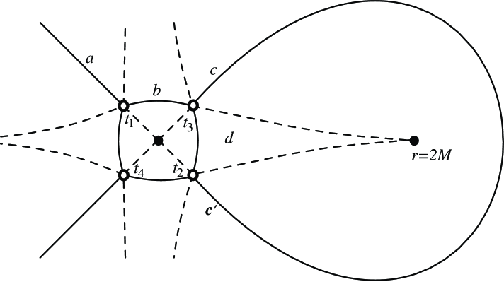
Figure 1: A schematic illustration of the Stokes (dashed) and anti-Stokes (solid) lines for the Schwarzschild problem in the complex $r$-plane. We have assumed that the frequency is large and purely imaginary. For frequencies with a small real part, the pattern of Stokes and anti-Stokes lines changes only slightly (cf. various figures in al ; gbs ). The open circles represent the four zeros of $Q^{2}$, while the filled circles are the two poles (at the origin and the event horizon, respectively). The outgoing-wave boundary condition at infinity is imposed on the anti-Stokes line labelled $a$. For $\omega=\alpha-i\beta$, with $[\alpha,\beta]>0$ this anti-Stokes line asymptotes to a straight line at an angle $\arctan\beta/\alpha$, i.e. in the first quadrant of the complex $r$-plane.

With the chosen phase of $Q$ the outgoing-wave solution at point $a$ is

$$\psi_{a}=f_{1}^{(t_{1})}$$ (33)

Since no Stokes lines cross this contour, this solution will not change in character along the anti-Stokes line that connects point $a$ with the zero $t_{1}$. This means that we can readily extend the solution to the vicinity of $t_{1}$. However, if we want to extend the solution to point $b$ on a neighbouring anti-Stokes line we must account for the Stokes phenomenon. With our choice of phase for $Q$, the function $f_{1}^{(t_{1})}$ is dominant on the Stokes line which we must cross in going from $a$ to $b$. This means that we will get

$$\psi_{b}=f_{1}^{(t_{1})}-if_{2}^{(t_{1})}$$ (34)

since the Stokes constant for a single well separated zero is $-i$ if we move around the zero in the clockwise direction. Changing the lower limit of integration to $t_{3}$ we get

$$\psi_{b}=e^{i\gamma_{13}}f_{1}^{(t_{3})}-ie^{-i\gamma_{13}}f_{2}^{(t_{3})}=-f_{1}^{(t_{3})}+if_{2}^{(t_{3})}$$ (35)

Now extending this solution to point $c$ we do not cross any anti-Stokes lines so $f_{1}$ remains dominant. Hence, at $c$ we obtain

$$\psi_{c}=-f_{1}^{(t_{3})}+2if_{2}^{(t_{3})}$$ (36)

Since we do not cross any Stokes lines in moving from $c$ to $c^{\prime}$, the linear combination (36) remains a valid solution. However, we need to note that the phase-integral is now evaluated along a contour that loops around the pole at $r=2M$. If we replace this integration contour by one that lies to the left of the pole, we get

$$\psi_{c^{\prime}}=-e^{i\Gamma}f_{1}^{(t_{3})}+2ie^{-i\Gamma}f_{2}^{(t_{3})}$$ (37)

where $\Gamma$ is the integral of $Q$ along a contour encircling the pole at $r=2M$ clockwise.

We now want to connect the solution to the point $d$. In order to do this we must first ensure that the lower limit of the phase-integrals is $t_{2}$. That is, we use

$$\psi_{c^{\prime}}=-e^{i(\Gamma+\gamma_{32})}f_{1}^{(t_{2})}+2ie^{-i(\Gamma-\gamma_{32})}f_{2}^{(t_{2})}=e^{i\Gamma}f_{1}^{(t_{2})}-2ie^{-i\Gamma}f_{2}^{(t_{2})}$$ (38)

When we step inside the large anti-Stokes lobe in Fig. 1 the dominance of $f_{1}$ and $f_{2}$ is interchanged. Then, crossing the first of the two Stokes lines inside this lobe we obtain

$$\psi_{d} = \left[e^{i\Gamma}+2e^{-i\Gamma}\right]f_{1}^{(t_{2})}-2ie^{-i\Gamma}f_{2}^{(t_{2})}=\left[e^{i\Gamma}+2e^{-i\Gamma}\right]e^{i\gamma{23}}f_{1}^{(t_{3})}-2ie^{-i\Gamma}e^{i\gamma{-23}}f_{2}^{(t_{3})}$$ (39)

$$= -\left[e^{i\Gamma}+2e^{-i\Gamma}\right]f_{1}^{(t_{3})}+2ie^{-i\Gamma}f_{2}^{(t_{3})}$$

Connecting this solution back to $c$, again crossing a Stokes line where $f_{1}$ is subdominant, we get (using a bar on $c$ to denote the fact that we have encircled the pole at the origin)

$$\psi_{\bar{c}}=-\left[e^{i\Gamma}+4e^{-i\Gamma}\right]f_{1}^{(t_{3})}+2ie^{-i\Gamma}f_{2}^{(t_{3})}$$ (40)

Now reversing our steps and connecting this solution to $b$ we get

$$\psi_{\bar{b}} = -\left[e^{i\Gamma}+4e^{-i\Gamma}\right]f_{1}^{(t_{3})}-i\left[e^{i\Gamma}+2e^{-i\Gamma}\right]e^{-i\Gamma}f_{2}^{(t_{3})}$$ (41)

$$= -\left[e^{i\Gamma}+4e^{-i\Gamma}\right]e^{i\gamma_{31}}f_{1}^{(t_{1})}-i\left[e^{i\Gamma}+2e^{-i\Gamma}\right]e^{-i\gamma_{31}}f_{2}^{(t_{1})}$$

$$= \left[e^{i\Gamma}+4e^{-i\Gamma}\right]f_{1}^{(t_{1})}+i\left[e^{i\Gamma}+2e^{-i\Gamma}\right]f_{2}^{(t_{1})}$$

and (finally) returning to $a$ we have

$$\psi_{\bar{a}} = \left[e^{i\Gamma}+4e^{-i\Gamma}\right]f_{1}^{(t_{1})}+2i\left[e^{i\Gamma}+3e^{-i\Gamma}\right]f_{2}^{(t_{1})}$$ (42)

Comparing this solution to (33) we clearly must require that

$$e^{i\Gamma}+3e^{-i\Gamma}=0$$ (43)

in order for the two solutions to be the same. This would lead to

$$\psi_{\bar{a}}=e^{-i\Gamma}f_{1}^{(t_{1})}$$ (44)

from which we see that the clockwise monodromy of this solution is $e^{-i\Gamma}$.

Let us now perform the same analysis in the vicinity of the pole at $r=2M$. With our choice of phase for $Q$, the solution that represents “ingoing waves” near the event horizon is

$$\psi_{H}=\beta f_{2}^{(t_{3})}$$ (45)

For this solution it is trivial to show that the clockwise monodromy is (again) $e^{-i\Gamma}$.

Since a necessary condition for the two solutions (33) and (45) to represent the same global solution to the problem is that they have the same monodromy, we conclude that (43) is the appropriate WKB condition for highly damped QNM solutions.

Finally, using the fact that

$$\Gamma=\oint Qdr=-2\pi i\mathop{Res}_{r=2M}Q=-4\pi i\omega M$$ (46)

our WKB condition can be written

$$e^{2i\Gamma}=e^{8\pi\omega M}=-3$$ (47)

and it immediately follows that

$$\omega M={1\over 8\pi}\ln 3-{i\over 4}\left(n+{1\over 2}\right)\quad\mbox{ as }n\to\infty$$ (48)

This is the desired final answer, in complete agreement with motl ; motl2 ; mvdb . Of course, it is worth noting that our derivation is conceptually very simple as it only appeals to basic WKB principles.

It is interesting to discuss other classes of black hole perturbations. In order to do this we note that, had we not used the particular value $\gamma=\pi$ in our derivation, we would have arrived at the condition

$$e^{8\pi\omega M}=-1-2\cos 2\gamma$$ (49)

We can easily use this condition to determine the asymptotic QNMs for electromagnetic waves.

In the case of electromagnetic waves propagating in the Schwarzschild geometry the relevant effective potential is

$$V=l(l+1){\Delta\over r^{4}}$$ (50)

From this we find, using (16) and (28), that

$$Q^{2}\approx{r^{2}\over 4M^{2}}\left[\omega^{2}-{4M^{2}\over r^{4}}\right]$$ (51)

The topology of the problem is still represented by Figure 1, and given (31) we find that

$$\int Qdr\approx\pm\int{r\over 2M}\left[\omega^{2}-{4M^{2}\over r^{4}}\right]^{1/2}dr=\pm{\pi\over 2}$$ (52)

Hence, we have $\gamma=\pi/2$ and it follows immediately from (49) that the real part of the QNM frequencies vanishes asymptotically.

IV The Reissner-Nordström problem

Having verified the known result for Schwarzschild black holes we will now consider the QNMs of the Reissner-Nordström geometry. This problem has recently been discussed by several authors, see motl2 ; bk ; neitzke , but the implications of the results still seem far from clear. The Reissner-Nordström problem is more complicated than the Schwarzschild one because of the presence of the inner horizon as well as two additional zeros of the relevant $Q^{2}$. Nevertheless, the analysis proceeds almost exactly as in the previous section.

In the case of charged black holes, one still only needs to consider axial perturbations. Just as in the Schwarzschild case the axial and polar perturbations are isospectral chandra . For axial perturbations one has two distinct effective potentials, cf. aas ,

$$V_{i}={\Delta\over r^{2}}\left[{l(l+1)\over r^{2}}-{\beta_{i}\over r^{3}}+{4q^{2}\over r^{4}}\right]$$ (53)

where

$$\beta_{1,2}=3M\mp[M^{2}+4(l-1)(l+2)q^{2}]^{1/2}$$ (54)

In the Schwarzschild limit ($q\to 0$) these potentials approach pure electromagnetic ($V_{1}$) and gravitational ($V_{2}$) perturbations, respectively. In the general charged case, the solution corresponds to coupled electromagnetic and gravitational waves. That this should be the case is natural since oscillations of a charged gravitational field will inevitably generate electromagnetic waves, and vice versa. Note that the $q\to 0$ limit is, in fact, singular due to the coalescences of poles and zeros that change the character of the function $Q^{2}$, cf. Figs. 1 and 2.

IV.1 Evaluating the phase-integrals

When $q\neq 0$ the function $R$ has three second order poles and six zeros regardless of whether we consider $V_{1}$ or $V_{2}$. Furthermore, just as in the Schwarzschild case, the zeros all approach the origin of the complex $r$-plane when $|\omega|\to\infty$. Again expanding in a power series we find

$$R\approx{r^{4}\over q^{4}}\left[\omega^{2}-{6q^{4}\over r^{6}}\right]\approx-{6\over r^{2}}$$ (55)

in the immediate neighbourhood of $r=0$. The leading order behaviour is the same for both classes of perturbations ($V_{1}$ and $V_{2}$). Hence, our analysis will hold for both sets of perturbations and the final result will be identical in the two cases.

Repeating the argument from the previous section one can show that the choice (28) still leads to the WKB solutions having the behaviour expected of the exact solutions near $r=0$. Thus we will use

$$Q^{2}\approx{r^{4}\over q^{4}}\left[\omega^{2}-{25q^{4}\over 4r^{6}}\right]$$ (56)

As in the previous section we will need the phase-integral connecting neighbouring zeros of $Q^{2}$. That is, we require

$$I=\int Qdr\approx\pm\int{r^{2}\over q^{2}}\left[\omega^{2}-{25q^{4}\over 4r^{6}}\right]^{1/2}dr$$ (57)

Letting $y=2\omega r^{3}/5q^{2}$, and using two neighbouring zeros of $Q^{2}$ as limits, the integral becomes identical to that of the Schwarzschild problem (apart from a multiplicative factor), and we find

$$I=\pm{5\pi\over 6}$$ (58)

Yet again all the integrals we need are the same (up to sign). Chosing the phase of $Q$ as in the previous case, and labelling the zeros as in Fig. 2, we have

$$\gamma=-\gamma_{12}=-\gamma_{32}=\gamma_{43}=-\gamma_{54}={5\pi\over 6}\ .$$ (59)

Let us denote the integral along a contour that encircles the pole at $r_{+}$ (in the negative direction) by $\Gamma_{e}$. Then

$$\Gamma_{e}=\tilde{\gamma}_{25}+\gamma_{54}+\tilde{\gamma}_{43}+\gamma_{32}=\tilde{\gamma}_{25}+\tilde{\gamma}_{43}-2\gamma$$ (60)

where a tilde indicates that the integral is taken along an anti-Stokes lobe to the right of either the pole at the event horizon ($\tilde{\gamma}_{25}$) or the pole at the inner Cauchy horizon ($\tilde{\gamma}_{43}$), cf. Fig 2. Similarly, we define

$$\Gamma_{i}=-\tilde{\gamma}_{43}+\gamma_{43}=-\tilde{\gamma}_{43}+\gamma$$ (61)

These definitions allow us to write

$$\tilde{\gamma}_{43}=-\Gamma_{i}+\gamma$$ (62)

and

$$\tilde{\gamma}_{25}=\Gamma_{e}+\Gamma_{i}+\gamma$$ (63)

The two integrals $\Gamma_{e}$ and $\Gamma_{i}$ are readily evaluated using the residue theorem. We find

$$\Gamma_{e}=-2\pi i\mathop{Res}_{r=r_{+}}Q=-\pi i{\omega r_{+}^{2}\over\sqrt{M^{2}-q^{2}}}=-\pi i{\omega M\over\kappa}(1+\kappa)^{2}$$ (64)

where we have defined the dimensionless parameter

$$\kappa=\sqrt{1-{q^{2}\over M^{2}}}$$ (65)

The integral around the inner horizon is

$$\Gamma_{i}=-2\pi i\mathop{Res}_{r=r_{-}}Q=\pi i{\omega r_{-}^{2}\over\sqrt{M^{2}-q^{2}}}=\pi i{\omega M\over\kappa}(1-\kappa)^{2}$$ (66)

IV.2 The WKB condition for Reissner-Nordström QNMs

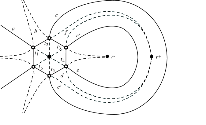
Figure 2: Stokes and anti-Stokes lines for Reissner-Nordström problem. Just as Fig. 1, this is a schematic picture based on a purely imaginary frequency. The three poles in the problem are represented by filled circles and correspond to, from left to right, the origin, the inner horizon and the event horizon. The six zeros of $Q^{2}$ are shown as open circles.

The pattern of Stokes and anti-Stokes lines for the Reissner-Nordström problem for $|\mbox{Im }\omega|>>|\mbox{Re }\omega|$ is shown in Figure 2. Introducing the outgoing-wave boundary condition on the appropriate anti-Stokes line (at point $a$ in Fig. 2), just as in the Schwarzschild problem, and then moving around the pole at $r=r_{+}$, taking full account of all involved Stokes phenomena (assuming the zeros are well isolated and can be treated individually), we arrive at the following WKB condition for highly damped QNMs

$$e^{2i\Gamma_{e}}=1-\left(1+e^{-2i\gamma}\right)\left(1+e^{2i\gamma}\right)\left(1+e^{-2i\Gamma_{i}}\right)$$ (67)

(the complete derivation is provided in the Appendix). Since we know that $\gamma=5\pi/6$ this becomes

$$e^{2i\Gamma_{e}}=1-2\left(1+\cos{5\pi\over 3}\right)\left(1+e^{-2i\Gamma_{i}}\right)=-2-3e^{-2i\Gamma_{i}}$$ (68)

which can be shown to be identical to the condition recently derived by Motl and Neitzke motl2 using matched asymptotics. That this condition agrees well with the numerical solution to the QNM problem, for various given overtones, has been shown by Berti and Kokkotas bk .

IV.3 Approaching the Schwarzschild limit

It is interesting to consider what happens when the black hole approaches the Schwarzschild limit, since (68) is clearly at variance with the result (47) for Schwarzschild black holes. For $|\omega|\to\infty$ then $q\to 0$, we have

$$\Gamma_{e}\approx-4\pi i\omega M\left(1+{q^{4}\over 16M^{4}}\right)$$ (69)

and

$$\Gamma_{i}\approx\pi i\omega M{q^{4}\over 4M^{3}}$$ (70)

Thus (68) predicts that we ought to have

$$e^{8\pi\omega M}=-5$$ (71)

Yet the Schwarzschild calculation predicted that the right-hand side should be $-3$! The reason for the discrepancy is, however, easy to explain. As we have already mentioned the Schwarzschild limit is singular. At our level of approximation one cannot move from the topology of Fig. 2 to that of Fig. 1 in a non-trivial way. This would require a uniform approximation involving the coalescence of two zeros and two poles.

The asymptotic behaviour of the QNMs of a charged black hole is always given by (68), and hence corresponds to the real part of the QNM frequencies approaching $\ln 5/8\pi$ in the limit of infinite damping. But there is also likely to be an intermediate regime in which the highly damped QNMs more resemble the Schwarzschild result, i.e. where Re $\omega M\approx\ln 3/8\pi$. As the Schwarzschild limit is approached, this latter regime tends to dominate, with the true Reissner-Nordström asymptotic behaviour being relevant only for extremely rapidly damped QNMs. That this is the case can be understood by the following argument: Let us consider a black hole with an infinitesimal charge and QNMs such that $|\mbox{Im }\omega M|>>|\mbox{Re }\omega M|$. The main difference between this problem and the Schwarzschild case is the presence of the double pole associated with the inner horizon $r_{-}$, and two additional zeroes of the function $R$, defined by (16). As the imaginary part of the QNMs increases, all six zeros of $R$ move towards the double pole at the origin. Our analysis of the problem is only relevant when the topology is that illustrated in Fig. 2, i.e. when the pole at $r_{-}$ lies outside the circle on which the six zeroes are located. For infinitesimally charged black holes there will also exist a regime where the topology of the the four zeroes already present in the Schwarzschild case are essentially unchanged. For this to be true, we need to have

$$|t|\approx\left(M/\omega\right)^{1/2}$$ (72)

At the same time the pole at $r_{-}$, and the two additional zeroes that come into existence when the black hole attains charge (and which emerge from the origin together with $r_{-}$), must lie well inside the circle of “Schwarzschild” zeroes. This corresponds to

$$|r_{-}|<<|t|\rightarrow q^{2}<<2M\left(M/\omega\right)^{1/2}$$ (73)

If these conditions are met one would expect the QNMs to be similar to the Schwarzschild ones. Figure 3 is a schematic illustration of the two regimes for highly damped Reissner-Nordström QNMs. Even though it is easy to explain the behaviour in principle, it is not straightforward to extend our analysis into a consistent scheme for calculating the QNMs in the intermediate regime. The main reason for this is the need to evaluate the phase-integral $\gamma$. In the intermediate regime we can no longer make use of the power series expansion around the origin that led to (29). Such an expansion is only valid up to the nearest pole, i.e. $r_{-}$. Resolving this issue, and determining the QNMs also in this intermediate regime, may be an interesting problem but we do not consider it further here.

IV.4 Solving the QNM condition

In order to discuss the solutions to the Reissner-Nordström QNM condition, it is useful to rewrite (68) as

$$e^{8\pi\omega M}=-3-2e^{-2\pi\omega M(1-\kappa)^{2}/\kappa}$$ (74)

where we have used (64) and (66). From this we easily see that in the extremely charged case, as $\kappa\to 0$, we regain the Schwarzschild result neitzke . That is, we get

$$\mbox{Re }\omega M\to{\ln 3\over 8\pi}\quad\mbox{ as }q\to M$$ (75)

It is, however, not clear to what extent this result is relevant. After all, the extreme Reissner-Nordström limit is singular in the sense that the two poles at $r_{\pm}$ coalesce as $q\to M$. This means that the topology is no longer that illustrated in Fig. 2, and hence the extreme Reissner-Nordström case would require a separate analysis.

In order to analyse the general case, we introduce

$$y=8\pi\omega M\qquad\mbox{ and }\quad k={(1-\kappa)^{2}\over 4\kappa}$$ (76)

The condition can then be written as

$$e^{y}=-3-2e^{-ky}\ .$$ (77)

In general, this condition must be solved numerically. One way to do this is to first separate the real and imaginary parts of the equation. Letting $y=\alpha-i\beta$ we obtain the two equations

$$e^{\alpha}\cos\beta = -3-2e^{-k\alpha}\cos k\beta$$ (78)

$$e^{\alpha}\sin\beta = 2e^{-k\alpha}\sin k\beta$$ (79)

These equations are very useful. First of all we see that, if we want the solution to be periodic in $\beta$, we must require simultaneously

$$\beta\to\beta+2n\pi\quad\mbox{ and }\quad\quad k(\beta+2n\pi)=k\beta+2m\pi$$ (80)

where $n$ and $m$ are integers. That is, periodicity in Im $\omega$ is only possible if

$$k={m\over n}$$ (81)

Since $0\leq k\leq\infty$ we see that we will pass through all (positive) rational values for $k$ as the charge of the black hole is varied. Hence, there will be an infinite set of cases where the solution is periodic in the imaginary part. However, whenever $k$ is not a rational number, the spectrum ceases to be periodic in the imaginary part. This is a significant observation because it illustrates that the asymptotic Reissner-Nordström spectrum is generally very different from that of a Schwarzschild black hole. One might wonder if the inclusion of higher order terms in the approximation would reimpose periodicity in Im $\omega$ for irrational values of $k$. However, this seems unlikely since it would require a surprising “conspiracy” between these terms. The difficulty (due to truncation error) of representing exactly rational numbers would pose significant challenges for a numerical verification of this result.

For $m$ and $n$ integers we can introduce $z=e^{y/n}$ to get

$$z^{n+m}+3z^{m}+2=0$$ (82)

which obviously has $n+m$ roots (one of these polynomial cases was discussed in neitzke ). These roots lead to

$$8\pi\omega M=y=n\ln|z|+in\arg z+2np\pi i\quad p=0,1,2,...$$ (83)

Only some of these roots will be compatible with the derivation of our WKB condition since we assumed that Re $\omega M\geq 0$ at the outset. The permissible roots correspond to the smallest basis set required to recontruct the spectrum. Repetitions of these roots on other sheets of $z$ (different $k$), for large $p$ generate the asymptotic spectrum, cf. figure 3. Hence, it is interesting to consider some of these polynomial solutions. In Table 1 we give the roots that are compatible with the derivation of our QNM condition for some selected values of $k=m/n$.

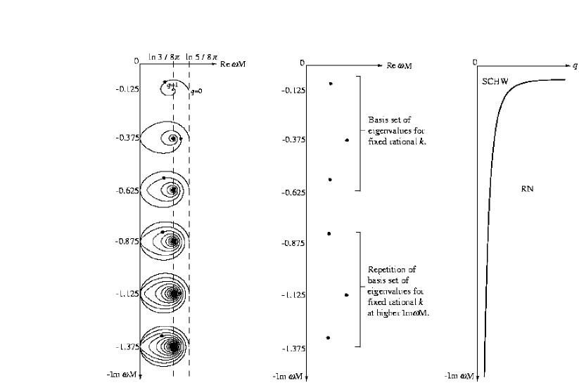
Figure 3: Left panel: A schematic illustration of the behaviour of the first few solutions to the Reissner-Nordström QNM condition (68). As the charge is increased the QNM frequencies spiral towards $\ln 3/8\pi-(2p+1)i/8$. The figure illustrates how the spirals tighten with increasing damping. Generally, the asymptotic QNMs correspond to the high damping limit of the figure. Middle panel: In the case of fixed rational $k=m/n$, the spectrum is divided into repetitions of basis sets of eigenvalues from low-lying states (indicated by dots). The number of modes in the basis set increases with $n$. For irrational $k$ this periodicity is destroyed. Right panel: A schematic illustration of the two asymptotic regimes of the Reissner-Nordström problem, RN and SCHW in the figure. In the limit of infinite damping the QNMs are determined by (68), but there also exists an intermediate “Schwarzschild-like” regime . The boundary between the two regimes is (roughly) given by $q^{2}\approx 2M\left(M/\omega\right)^{1/2}$.

The data given in Table 1 provide the basis needed to generate the asymptotic QNM spectrum in the simplest periodic cases. As shown in the table, there are $n$ distinct QNMs in each basis set. These yield the asymptotic spectrum for large values of $p$, cf. (83). These results are only valid in the regime where the topology of the problem is that shown in Figure 2. From our discussion of the Schwarzschild limit above, we deduce that this is the case when

$$|\mbox{Im }\omega M|>>4(M/q)^{4}$$ (84)

It is relevant to ask if there are any values of $k$ for which we have purely imaginary frequencies. One can show that $\alpha=0$ is only compatible with (78) and (79) provided that

$$\sin\beta=0\quad\mbox{ and }\cos\beta=-1$$ (85)

That is, we must have

$$k={2m+1\over 2n+1}$$ (86)

where $n$ and $m$ are integers. One of these roots (for $m=1$ and $n=3$) is present in Table 1. These purely imaginary solution may be the cause of some confusion because it is debatable whether they are compatible with the assumptions made in the derivation of our QNM condition. In particular, it is not clear to what extent these solutions are relevant for a discussion of “purely outgoing wave” solutions. Furthermore, one has to be careful because only some of the purely imaginary roots belong to modes that can be traced back to a Schwarzschild QNM. The condition (68) was derived assuming that the real part of the frequency was positive. Yet, a numerical solution of the condition also yields roots with a negative real part. These are not compatible with the underlying assumptions and should be discarded as unphysical. These unphysical roots also form spirals as $q$ is varied. Some of the purely imaginary roots of the polynomial belong to these presumed unphysical solutions.

By complementing the polynomial roots with a numerical solution of (68), cf. Figure 3, we can further elucidate the behaviour of the asymptotic charged black hole QNMs. The numerical solutions illustrated in Figure 3 clearly show the spiral nature of the QNMs. Furthermore, we see that the number of times that each spiral touches the imaginary axis increases with the “order” of the mode. It is clear that, as Im $\omega M\to-\infty$ the spirals tighten, i.e. the QNM frequency becomes exponentially sensitive to variations in $q$. Whether this is a hint that the problem becomes probabilistic in the limit of infinite damping is not clear.

$m$	$n$	$q/M$	$\omega M$
$\infty$	—	$1^{\dagger}$	$\ln 3/8\pi-i/8=0.04371-i/8$
8	1	0.9996	$0.04372-i/8$
7	1	0.9994	$0.04370-i/8$
6	1	0.9993	$0.04375-i/8$
5	1	0.9990	$0.04360-i/8$
4	1	0.9984	$0.04403-i/8$
7	2	0.9980	$0.04374-0.12556i$	$0.04374-0.37444$
3	1	0.9974	$0.04263-i/8$
8	3	0.9968	$0.04311-0.12364i$	$0.04499-3i/8$	$0.04311-0.62636i$
5	2	0.9965	$0.04392-0.12334i$	$0.04392-0.37666i$
7	3	0.9960	$0.04483-0.12348i$	$0.04128-3i/8$	$0.04483-0.62652i$
2	1	0.9949	$0.04623-i/8$
7	4	0.9936	$0.04634-0.12707i$	$0.04129-0.37873i$	$0.04129-0.61127i$	$0.04634-0.87293i$
5	3	0.9931	$0.04607-0.12790i$	$0.03788-3i/8$	$0.04607-0.62290i$
3	2	0.9919	$0.04484-0.12969i$	$0.04484-0.37031i$
4	3	0.9903	$0.04222-0.13140i$	$0.04860-3i/8$	$0.04222-0.61860i$
5	4	0.9893	$0.04008-0.13200i$	$0.04815-0.37830i$	$0.04815-0.62170i$	$0.04008-0.86800i$
1	1	0.9852	$\ln 2/8\pi-i/8$
3	4	0.9780	$0.03849-0.11227i$	$0.05121-0.36969i$	$0.05121-0.63031i$	$0.03849-0.88773i$
2	3	0.9743	$0.04193-0.11162i$	$0.05331-3i/8$	$0.04193-0.63838i$
1	2	0.9634	$0.04817-0.11199i$	$0.04817-0.38801i$
1	3	0.9428	$0.05391-0.11419i$	$-3i/8$	$0.05391-0.63581i$
1	4	0.9242	$0.05664-0.11598i$	$0.03493-0.35261i$	$0.03493-0.64739i$	$0.05664-0.88402i$
—	$\infty$	$0^{\dagger}$	$\ln 5/8\pi-i/8=0.06404-i/8$

Table 1: A sample of roots in cases where the asymptotic spectrum is periodic in the imaginary part. These roots for the basis sets out of which the highly damped QNM spectrum is constructed. ^†We include the predictions of (68) for both the Schwarzschild limit and the extremely charged black hole limit despite these limits being “singular”, cf. the discussion in the main text.

V Discussion

In this paper we have provided WKB results for highly damped quasinormal modes of Schwarzschild and Reissner-Nordström black holes. In the Schwarzschild case, we have verified previous results for gravitational perturbations. In particular, we have provided a clear derivation of the fact that the real part of the quasinormal mode frequencies approaches Re $\omega M=\ln 3/8\pi$ asymptotically, cf. Eq. (48). We have also shown that the real part of the asymptotic modes vanishes for electromagnetic waves. For Reissner-Nordström black holes we have verified the QNM condition recently obtained by Motl and Neitzke motl2 , our Eq. (68). In addition, we have shown that this result holds to leading order, not only for the class of perturbations that limits to pure gravitational waves as $q\to 0$, but also for the class that limits to pure electromagnetic waves. That these two classes of perturbations are isospectral for highly damped modes was not known previously. Perhaps the most relevant result concerns the fact that the asymptotic QNM frequencies of charged black holes are in general not periodic in the imaginary part. This means that the asymptotic spectrum is significantly more complicated than in the Schwarzschild case. We have also explained the breakdown of the analysis in the Schwarzschild limit. The WKB approach that we have used should be applicable to many similar problems. In particular, it should be possible to use our approach to study the Kerr problem bk ; hod2 .

Before we conclude the paper, let us return to the question of a possible link between the QNMs and quantum gravity. Do the present results shed further light on this association, or does it now seem as if Hod’s original suggestion was based on a misleading coincidence? Unfortunately, the available results do not provide a clear answer to this question. Hence, we conclude this paper with some speculations.

First, the original result for gravitational perturbations of Schwarzschild black holes holds. If one accepts the proposed correspondence between the QNM frequencies and a “transition energy” $\Delta M$ one finds that the quantum of area should be $\Delta A=4\ln 3$. How do results for other perturbing fields fit into this picture? For example, what about the fact that the real part of the electromagnetic QNMs vanishes asymptotically? Although interesting in its own right, this result is probably not relevant for the discussion. A natural reason for this would be the fundamental difference between gravitational and electromagnetic perturbations of Schwarzschild black holes. While electromagnetic perturbations correspond to waves propagating in a fixed background, the gravitational waves represent oscillations of the spacetime itself. It would perhaps not be surprising if results for the former problem tell us little about the quantum levels of the black hole. Could a study of massive fields allow us to make progress?

The situation is even more complicated when we turn to the Reissner-Nordström problem. How can our results be understood? At first sight it would be tempting to suggest that the generally nonperiodic nature of the asymptotic QNM spectrum, with no unique Re $\omega M$, provides an argument against any quantum correspondence. However, this conclusion might be premature. One reason for this is that a general perturbation of a Reissner-Nordström black hole corresponds to a mixture of electromagnetic and gravitational waves. Would it be too surprising if this mixing were to prevent a simple correspondence argument? Moreover, we have the unexpected result that we retain the same result for the asymptotic QNMs in both the Schwarzschild and the extreme Reissner-Nordström limits. Is this telling us something profound or is it (again) a mere coincidence?

Suppose we accept the association between the asymptotic QNMs and the quantum area $\Delta A$ . What would this imply for a general charged black hole? The area of a charged black hole is given by

$$A=4\pi r_{+}^{2}$$ (87)

From this we readily get (using $\kappa$ as defined in Eq. (76))

$$\Delta A={8\pi M(1+\kappa)^{2}\over\kappa}\Delta M-{8\pi q(1+\kappa)\over\kappa}\Delta q={8\pi r_{+}^{2}\over M\kappa}\Delta M-{8\pi qr_{+}\over M\kappa}\Delta q$$ (88)

From this relation it is clear that, in general, knowledge of $\Delta M$ alone is not sufficient to “predict” $\Delta A$. We also need to disentangle the electromagnetic waves from the gravitational ones.

In the absence of more information we can play a simple game. Let us assume that $\Delta A$ is indeed universal and thus remains as in the Schwarzschild case ($=4\ln 3$). Then we can infer from (88) that

$$q\Delta q=r_{+}\Delta M-{\kappa M\ln 3\over 2\pi r_{+}}$$ (89)

If we associate an “energy” with a given oscillation frequency we have $\Delta M=\omega$ and thus

$$q\Delta q=r_{+}\omega-{\kappa M\ln 3\over 2\pi r_{+}}$$ (90)

From this relation we can, given any QNM, compute the value of $\Delta q$ required for us to obtain the same unique $\Delta A$. In the particular case of extremely charged black holes we would get (since $\kappa\to 0$ as $q\to M$)

$$\Delta q=r_{+}\omega=\omega M={\ln 3\over 8\pi}=\Delta M$$ (91)

We can also use (90) as a measure of the degree to which a perturbation is “electromagnetic” or “gravitational”. To what extent this kind of analysis makes sense is, of course, an open question.

Appendix: The Reissner-Nordström calculation

In this Appendix we provide the complete derivation of the WKB condition for highly damped Reissner-Nordström QNMs.

The outgoing-wave solution at point $a$ is

$$\psi_{a}=f_{1}^{(t_{1})}$$ (92)

Moving around the pole at $r=r_{+}$, cf. Fig. 2, taking full account of all involved Stokes phenomena (assuming that the zeros are well isolated) we get

$$\psi_{b}=f_{1}^{(t_{1})}-if_{2}^{(t_{1})}=e^{-i\gamma}f_{1}^{(t_{2})}-ie^{i\gamma}f_{2}^{(t_{2})}$$ (93)

$$\psi_{c}=e^{-i\gamma}f_{1}^{(t_{2})}-i\left[e^{i\gamma}+e^{-i\gamma}\right]f_{2}^{(t_{2})}$$ (94)

$$\psi_{c^{\prime}}=e^{i(\Gamma_{e}+\Gamma_{i})}f_{1}^{(t_{5})}-i\left[1+e^{-2i\gamma}\right]e^{-i(\Gamma_{e}+\Gamma_{i})}f_{2}^{(t_{5})}$$ (95)

where we have used (63), and then

$$\psi_{d} = \left\{e^{i(\Gamma_{e}+\Gamma_{i})}+\left[1+e^{-2i\gamma}\right]e^{-i(\Gamma_{e}+\Gamma_{i})}\right\}f_{1}^{(t_{5})}-i\left[1+e^{-2i\gamma}\right]e^{-i(\Gamma_{e}+\Gamma_{i})}f_{2}^{(t_{5})}$$ (96)

$$= \left\{e^{i(\Gamma_{e}+\Gamma_{i}-\gamma)}+e^{-i\gamma}\left[1+e^{-2i\gamma}\right]e^{-i(\Gamma_{e}+\Gamma_{i})}\right\}f_{1}^{(t_{4})}-i\left[e^{i\gamma}+e^{-i\gamma}\right]e^{-i(\Gamma_{e}+\Gamma_{i})}f_{2}^{(t_{4})}$$

$$\psi_{e} = \left\{e^{i(\Gamma_{e}+\Gamma_{i})}+\left(1+e^{2i\gamma}\right)\left(1+e^{-2i\gamma}\right)e^{-i(\Gamma_{e}+\Gamma_{i})}\right\}e^{-i\gamma}f_{1}^{(t_{4})}$$ (97)

$$- i\left(1+e^{-2i\gamma}\right)e^{-i(\Gamma_{e}+\Gamma_{i}-\gamma)}f_{2}^{(t_{4})}$$

Moving around the pole at the inner horizon (to $e^{\prime}$), the solution does not change because no Stokes lines are crossed, but changing the lower limit of integration back to $t_{3}$ we get

$$\psi_{e^{\prime}} = \left\{e^{i\Gamma_{e}}+\left(1+e^{2i\gamma}\right)\left(1+e^{-2i\gamma}\right)e^{-i(\Gamma_{e}+2\Gamma_{i})}\right\}f_{1}^{(t_{3})}-i\left(1+e^{-2i\gamma}\right)e^{-i\Gamma_{e}}f_{2}^{(t_{3})}$$ (98)

Then

$$\psi_{f} = \left\{e^{i\Gamma_{e}}+\left(1+e^{-2i\gamma}\right)\left[1+\left(1+e^{2i\gamma}\right)e^{-2i\Gamma_{i}}\right]e^{-i\Gamma_{e}}\right\}f_{1}^{(t_{3})}-i\left(1+e^{-2i\gamma}\right)e^{-i\Gamma_{e}}f_{2}^{(t_{3})}$$ (99)

$$= e^{-i\gamma}\left\{e^{i\Gamma_{e}}+\left(1+e^{-2i\gamma}\right)\left[1+\left(1+e^{2i\gamma}\right)e^{-2i\Gamma_{i}}\right]e^{-i\Gamma_{e}}\right\}f_{1}^{(t_{2})}$$

$$- i\left[1+e^{-2i\gamma}\right]e^{-i(\Gamma_{e}-\gamma)}f_{2}^{(t_{2})}$$

$$\psi_{\bar{c}} = e^{-i\gamma}\left\{e^{i\Gamma_{e}}+\left(1+e^{-2i\gamma}\right)\left[1+e^{2i\gamma}+\left(1+e^{2i\gamma}\right)e^{-2i\Gamma_{i}}\right]e^{-i\Gamma_{e}}\right\}f_{1}^{(t_{2})}$$ (100)

$$- i\left(1+e^{-2i\gamma}\right)e^{-i(\Gamma_{e}-\gamma)}f_{2}^{(t_{2})}$$

$$\psi_{\bar{b}} = e^{-i\gamma}\left\{e^{i\Gamma_{e}}+\left(1+e^{-2i\gamma}\right)\left[1+e^{2i\gamma}+\left(1+e^{2i\gamma}\right)e^{-2i\Gamma_{i}}\right]e^{-i\Gamma_{e}}\right\}f_{1}^{(t_{2})}$$ (101)

$$+ ie^{-i\gamma}\left\{e^{i\Gamma_{e}}+\left(1+e^{-2i\gamma}\right)\left[1+\left(1+e^{2i\gamma}\right)e^{-2i\Gamma_{i}}\right]e^{-i\Gamma_{e}}\right\}f_{2}^{(t_{2})}$$

$$= Af_{1}^{(t_{1})}+iBf_{2}^{(t_{1})}$$

where

$$A=e^{i\Gamma_{e}}+\left(1+e^{-2i\gamma}\right)\left(1+e^{2i\gamma}\right)\left(1+e^{-2i\Gamma_{i}}\right)e^{-i\Gamma_{e}}$$ (102)

$$B = e^{-2i\gamma}\left\{e^{i\Gamma_{e}}+\left(1+e^{-2i\gamma}\right)\left[1+\left(1+e^{2i\gamma}\right)e^{-2i\Gamma_{i}}\right]e^{-i\Gamma_{e}}\right\}$$ (103)

$$= Ae^{-2i\gamma}-\left(1+e^{-2i\gamma}\right)e^{-i\Gamma_{e}}$$

Finally returning to the starting point $a$, we have

$$\psi_{\bar{a}}=Af_{1}^{(t_{1})}+i(A+B)f_{2}^{(t_{1})}$$ (104)

Thus we see that, in order for the coefficient of $f_{2}$ to vanish we must require

$$A+B=A+Ae^{-2i\gamma}-\left(1+e^{-2i\gamma}\right)e^{-i\Gamma_{e}}=0$$ (105)

That is, we should have

$$A=e^{-i\Gamma_{e}}$$ (106)

which is not too surprising given the result in the Schwarzschild case. As in that problem, one readily shows that the (clockwise) monodromy of the solution that is purely ingoing at the event horizon is also $e^{-i\Gamma_{e}}$. Hence, our calculation is consistent. Given the definition of $A$ the WKB condition for highly damped Reissner-Nordström QNMs becomes

$$e^{2i\Gamma_{e}}=1-\left(1+e^{-2i\gamma}\right)\left(1+e^{2i\gamma}\right)\left(1+e^{-2i\Gamma_{i}}\right)$$ (107)

References

- (1) B.F. Whiting, J. Math. Phys. 30 1301 (1989)
- (2) N. Andersson, Phys. Rev. D 55 468 (1997)
- (3) E.W. Leaver, Proc. Roy. Soc. London A 402 285 (1985)
- (4) N. Andersson, Proc. R. Soc. London A 439 47 (1992)
- (5) N. Andersson, Proc. R. Soc. London A 442 427 (1993)
- (6) H.P. Nollert and B.G. Schmidt, Phys. Rev. D 45 2617 (1992)
- (7) J.W. Guinn, C.M. Will, Y. Kojima and B.F. Schutz, Class. Quantum Grav. 7 L47 (1990)
- (8) H.P. Nollert, Phys. Rev. D 47 5253 (1993)
- (9) N. Andersson and S. Linnæus, Phys. Rev. D 46 4179 (1992)
- (10) N. Andersson, Class. Quantum Grav. 10 L61 (1993)
- (11) N. Andersson, M.E. Araújo and B.F. Schutz, Class. Quantum Grav. 10 735 (1993)
- (12) N. Andersson, M.E. Araújo and B.F. Schutz, Class. Quantum Grav. 10 757 (1993)
- (13) J.D. Bekenstein and V.F. Mukhanov, Phys. Lett. B 360 7 (1995)
- (14) A. Ashtekar, J. Baez, A. Corichi and K. Krasnov, Phys. Rev. Lett. 80 904 (1998)
- (15) A. Ashtekar, Quantum geometry in action: Big bang and black holes preprint maths-ph/0202008
- (16) J.W. York, Phys. Rev. D 28 2929 (1983)
- (17) S. Hod, Phys. Rev. Lett. 81 4293 (1998)
- (18) O. Dreyer, Phys. Rev. Lett. 90 081301 (2003)
- (19) A. Corichi, Phys. Rev. D 67 87502 (2003)
- (20) A.P. Polychronakos, Area spectrum and quasinormal modes of black holes preprint hep-th/0304135
- (21) G. Kunstatter, Phys. Rev. Lett. 90 161301 (2003)
- (22) R.K. Kaul and S.K. Rama, Black hole entropy from spin one punctures preprint gr-qc/0301128
- (23) D. Birmingham, Asymptotic Quasinormal Frequencies of d-dimensional Schwarzschild Black Holes preprint hep-th/0306004
- (24) G.L. Gunter, Philos. Trans. Roy. Soc. 296 497 (1980); Erratum 301 705 (1981)
- (25) K.D. Kokkotas and B.F. Schutz, Phys. Rev. D 37 3378 (1988)
- (26) E.W. Leaver, Phys. Rev. D 41 2986 (1990)
- (27) N. Andersson, M.E. Araújo and B.F. Schutz, Phys. Rev. D. 49 2703 (1994)
- (28) L. Motl, An analytical computation of asymptotic Schwarzschild quasinormal frequencies preprint gr-qc/0212096
- (29) L. Motl and A. Neitzke, Asymptotic black hole quasinormal frequencies preprint hep-th/0301173
- (30) A. Maassen van den Brink, WKB analysis of the Regge-Wheeler equation down in the frequency plane preprint gr-qc/0303095
- (31) E. Berti and K.D. Kokkotas, Asymptotic quasinormal modes of Reissner-Nordström and Kerr black holes preprint hep-th/0303029
- (32) A. Neitzke, Greybody factors at large imaginary frequencies preprint hep-th/0304080
- (33) J. Heading, An introduction to phase-integral methods (Methuen, London, 1962)
- (34) N. Fröman and P.O. Fröman JWKB approximation: contributions to the theory (North-Holland, Amsterdam, 1965)
- (35) M.V. Berry and K.E. Mount, Reps. Prog. Phys 35 315 (1972)
- (36) S. Chandrasekhar, The Mathematical Theory of Black Holes (Clarendon Press, Oxford, 1983)
- (37) M.V. Berry, Proc. Roy. Soc A 422 7 (1989)
- (38) S. Hod, Phys. Rev. D. 67 81501 (2003)