Impact of densitized lapse slicings on evolutions of a wobbling black hole

Abstract

We present long-term stable and second-order convergent evolutions of an excised wobbling black hole. Our results clearly demonstrate that the use of a densitized lapse function extends the lifetime of simulations dramatically. We also show the improvement in the stability of single static black holes when an algebraic densitized lapse condition is applied. In addition, we introduce a computationally inexpensive approach for tracking the location of the singularity suitable for mildly distorted black holes. The method is based on investigating the fall-off behavior and asymmetry of appropriate grid variables. This simple tracking method allows one to adjust the location of the excision region to follow the coordinate motion of the singularity.

I Introduction

The accurate, long-term stable evolution of binary black hole spacetimes is one of the most important challenges in general relativity research. While the solution of the relativistic two-body problem is highly relevant from an academic point of view, its importance is further enhanced by the need of such simulations for predicting the resulting gravitational wave emission. This will not only improve the chances of detecting gravitational waves but also be essential when it comes to the astrophysical interpretation of the measured wave patterns.

Early black hole evolutions (see e.g. Anninos et al. (1995a); Cook et al. (1998); Brandt et al. (2000)) were based on the canonical ADM formulation Arnowitt et al. (1962); York (1979) of the Einstein field equations. The stability properties of these evolutions, however, were severely limited. It gradually became accepted among the community that the underlying problems were not merely numerical in nature, but originated at least in part from the structure of the equations themselves. The striking success achieved in characteristic evolutions of single black hole spacetimes Gómez et al. (1998); Gómez and et. al. (1998) supports this view. As a result, numerous alternative 3+1 formulations have been constructed in recent years. The majority of these formulations are modified versions of the original ADM scheme. These alternative formulations either recast the Einstein field equations in explicitly hyperbolic form (see Kidder et al. (2001) and references therein) or exhibit some “hyperbolic flavor” such as the Baumgarte-Shapiro-Shibata-Nakamura (BSSN) system Shibata and Nakamura (1995); Baumgarte and Shapiro (1999).

In recent years, several of these new systems have demonstrated vastly improved stability properties, either in fully non-linear 3-dimensional black hole evolutions or suitably chosen test problems which isolate some of the particular difficulties faced in numerical relativity. Even though the question as to the optimal formulation of the Einstein equations remains as yet unanswered, the development of alternative 3+1 schemes has been one of the key driving forces underlying recent progress in numerical black hole evolutions.

In addition to the form used to recast the Einstein equations, considerable improvements have also been achieved in dealing with spacetime singularities inevitably present in such simulations. One approach, commonly known as singularity avoidance, foliates the spacetime in such a way that the evolution of the code is basically frozen near the singularity. As originally implemented, singularity avoidance methods enjoyed rather limited success, mainly due to the ‘grid-stretching’ effect — the increase of the proper separation between neighboring grid-points. The problem of grid-stretching has been alleviated to some extent by the introduction of a non-zero shift vector Alcubierre et al. (2003a). It is not clear, however, whether this approach will be able to sustain evolutions for the dynamical time-scales that are needed.

An alternative treatment, often attributed to a suggestion by Unruh (quoted in Thornburg (1987)), is based on the cosmic censorship conjecture. Cosmic censorship states that a spacetime singularity will be surrounded by a causal boundary, the black hole horizon. Physical information contained within this boundary cannot escape. Thus, in principle, one can get away with murder and excise a region inside the event horizon containing the black hole singularity, without affecting computations in the exterior. This technique, known as black hole excision or the apparent horizon boundary condition, has become very popular in recent years and has been implemented in a number of cases Seidel and Suen (1992); Anninos et al. (1995b); Marsa and Choptuik (1996); Scheel et al. (1997); Cook et al. (1998); Gómez et al. (1998); Brandt et al. (2000); Alcubierre et al. (2001); Yo et al. (2001); Alcubierre and Brügmann (2001); Shoemaker et al. (2003); Calabrese et al. (2003). It is important to note, however, that the causal boundary strictly applies to physical information only. Unless one can guarantee that all characteristic speeds of the evolved fields (physical and unphysical) lie within the light cone (for example by using an explicitly hyperbolic formulation), gauge modes may well leave the black hole interior. While these modes are not supposed to affect the physical results in the exterior evolution, they may have a significant impact on the numerical stability. The success of the excision technique as applied to non-manifestly-hyperbolic systems of equations is therefore by no means a foregone conclusion and needs to be demonstrated explicitly for the application at hand.

Earlier implementations of black hole excision were still based on the ADM scheme and frequently made use of causal-differencing and/or apparent horizon locking coordinates Cook et al. (1998); Seidel and Suen (1992); Anninos et al. (1995b). Aside from demonstrating the feasibility of the method, these simulations led to improved evolutions of single black hole spacetimes as compared with techniques based on singularity avoiding slicing conditions. These codes were, however, still subject to the fundamental limitations of the ADM formulation. In more recent times, excision has been combined with alternative formulations of the field equations and more general classes of gauge conditions. The resulting evolutions have been able to reach the first major goal on the way toward solving the binary black hole problem, namely the evolution of single, stationary black hole spacetimes in three dimensions for arbitrary times Alcubierre and Brügmann (2001); Yo et al. (2002); Gómez et al. (1998). In addressing dynamic black hole scenarios, one may attempt to absorb part or all of the black hole movement by choosing appropriate coordinates such as co-rotating coordinates in the case of an in-spiraling binary black hole Brady et al. (1998). However, it is unclear how such a treatment will be possible, in particular in the later stages just before the merger, without introducing a considerable degree of grid-stretching. It is unlikely, therefore, that such dynamic simulations can be achieved without an excision region that can adjust dynamically to mask the black hole singularity as it moves through the computational domain. In the words of Ref. Scheel et al. (1997), “a key milestone in three-dimensional black hole simulations is the ability to stably move a hole through the numerical grid”.

In characteristic formulations, long-term stable evolutions using a dynamic excision region have been achieved as early as 1998 for the case of a wobbling black hole Gómez and et. al. (1998). In 3+1 formulations, to our knowledge, the earliest attempts were performed by Cook et al. (1998), who managed to track a boosted black hole through the grid for 60 $M$ ( where $M$ is the mass of the black hole). Further applications of dynamic singularity excision include grazing collisions of black holes Brandt et al. (2000) and the evolution of a scalar field in a static or boosted Kerr-Schild black hole background Yo et al. (2001). In Shoemaker et al. (2003), a dynamic scenario was simulated by evolving a single black hole in ingoing-Eddington-Finkelstein (iEF) coordinates transformed to a coordinate system in which the coordinate location of the singularity traced out bouncing or circular paths on the coordinate grid. As the excision region is moved across the numerical grid in such evolutions, one will inevitably encounter previously excised grid points which reemerge into the evolved domain and thus need to be filled with valid data for the grid variables. In evolutions with dynamic excision, this is commonly done via extrapolation from neighboring grid points. The motivation for this procedure arises from the same causal considerations underlying the singularity excision mentioned above and is subject to the same reservations for non-manifestly-hyperbolic evolution systems. Several extrapolation techniques have been studied in Yo et al. (2001), where the stability properties of the ensuing evolutions are found to be rather insensitive to the precise details of the scheme.

In this paper, we expand directly on the work of Shoemaker et al. (2003) (referred to as Paper I from now on) where third-order extrapolation was used for the population of reemerging grid points. The resulting dynamic excision enabled these authors to evolve non-boosted black holes traveling on circular or bouncing trajectories for about $130\,M$. While such evolution times represent considerable progress on previous dynamic simulations, they do not meet the requirements for simulations of in-spiraling binary black holes. There remains, thus, the fundamental question of whether the dynamic excision techniques currently under consideration are in principle capable of handling long-term stable evolutions of moving black holes. Addressing this question is one of the main goals of this paper. We demonstrate how the lifetime of the dancing or wobbling black hole evolutions of Paper I can be extended to at least several thousands of $M$ by prescribing the slicing condition in terms of the densitized lapse as opposed to the lapse function itself. This also confirms the belief expressed in Paper I that the gauge conditions were a crucial factor in limiting the stability properties of the code. We further present a simple and very efficient mechanism by which our excision region was able to track the black hole movement by merely analyzing the updated numerical data, with no prior knowledge of the black hole trajectory. This mechanism analyzes the fall-off behavior of certain grid variables near the black hole singularity and provides us with an alternative at negligible computational cost to more commonly used apparent horizon tracking methods. This method for tracking singularities is suitable for situations in which the black hole is mildly distorted.

The numerical code used for the evolutions presented in this paper is the Maya code; details of the code can be found in Paper I. The code is based on the BSSN formulation Shibata and Nakamura (1995); Baumgarte and Shapiro (1999); we will not repeat the BSSN equations here — see e.g. Alcubierre et al. (2003a). Whenever we encounter conformally transformed quantities, we will distinguish them by a “hat” from physical quantities. Latin and Greek indices will run from 1 to 3 and 0 to 3 respectively. We define the order of an extrapolation scheme as the order of the polynomial used.

The paper is organized as follows. We describe and motivate in Sec. II the use of a densitized lapse for our numerical evolution. The numerical results together with convergence tests will be presented in Sec. III. In Sec. IV, we describe the simple scheme used in our evolutions for tracking the black hole singularity. We conclude in Sec. V with a discussion of our results.

II Introducing a densitized lapse

Under the canonical 3+1 decomposition of the Einstein equations, the line element is given by

$$ds^{2}=-\alpha^{2}dt^{2}+\gamma_{ij}(dx^{i}+\beta^{i}dt)(dx^{j}+\beta^{j}dt),$$ (1)

where the 3-metric $\gamma_{ij}$ describes the geometry of the space-like slices. The lapse function $\alpha$ relates the separation in proper time between two space-like slices to their difference $dt$ in coordinate time, and the shift vector $\beta^{i}$ determines how one identifies points with identical spatial coordinates on neighboring spatial hypersurfaces. For recasting the Einstein equations in a 3+1 form, it is convenient to also introduce the extrinsic curvature

$$K_{ij}=-\frac{1}{2\alpha}(\partial_{t}-\mathcal{L}_{\beta})\gamma_{ij},$$ (2)

where $\mathcal{L_{\beta}}$ denotes the Lie derivative along the shift vector. The extrinsic curvature describes the embedding of the 3-dimensional spatial slices in 4-dimensional spacetime. The 3+1 Einstein equations fall into two categories, 12 evolution equations for $\gamma_{ij}$ and $K_{ij}$, and 4 constraint equations (the Hamiltonian and momentum constraints). The majority of formulations of the Einstein field equations, and in particular the BSSN formulation we use for our code, are based on this decomposition but introduce various modifications, such as conformal decompositions, promoting auxiliary variables to fundamental status and combining the evolution and constraint equations to obtain systems with different mathematical and numerical properties.

The gauge functions $\alpha$ and $\beta^{i}$, on the other hand, represent the coordinate or gauge freedom of general relativity and can be chosen arbitrarily without affecting the physical spacetime. Their choice does, however, have a crucial impact on the performance of a numerical scheme used to evolve the Einstein equations. Since the evolution of the gauge variables is not determined by the Einstein equations, one needs to introduce a recipe to determine the the lapse and shift. Such gauge conditions can in principle be divided into three types (see for example Khokhlov and Novikov (2002)). Fixed gauge conditions are those for which $\alpha$ and $\beta^{i}$ are given functions of the spacetime coordinates $x^{\alpha}$. Algebraic conditions, on the other hand, are such that the lapse and shift are allowed to also depend on other evolved variables, such as $\gamma$, $K$ or derivatives of $\gamma_{ij}$. Finally, one may construct $\alpha$ and $\beta$ from solutions of differential equations (elliptic, parabolic or hyperbolic). This type is sometimes referred to as differential gauge conditions. Examples are minimal distortion shift and maximal slicing. A subclass of algebraic gauge conditions will be of particular importance for this work.

For the present work, we will only consider a fixed gauge condition for the shift vector; that is, the shift vector will be given by the exact solution for a single, non-rotating black hole in iEF coordinates. As mentioned before, in Paper I we also used a fixed gauge condition for the lapse function. The objective now is to replace this with an algebraic condition. In particular the algebraic lapse we consider is

$$\alpha=\gamma^{n/2}\,q=e^{6n\phi}\,q,$$ (3)

where $\phi$ is the conformal factor relating the physical metric $\gamma_{ij}$ to the conformal metric $\hat{\gamma}_{ij}$ such that

$$\gamma_{ij}=\gamma^{1/3}\hat{\gamma}_{ij}=e^{4\phi}\,\hat{\gamma}_{ij}\,.$$ (4)

We emphasize that in Eq. (3), $q$ replaces the lapse $\alpha$ as the independent variable. Notice that because $\alpha$ is a true scalar, $q$ is a density of weight $-n$, hence the name densitized lapse.

Such a densitized lapse or a generalized version thereof has played a crucial rule in the development of various hyperbolic formulations of Einstein’s field equations. For example Kidder et al. Kidder et al. (2001) find the use of a densitized version of the lapse necessary for obtaining strong hyperbolicity. In particular these authors obtain exclusively physical characteristic speeds for the case corresponding to $n=1$ in our Eq. (3). Similarly, Frittelli and Reula Frittelli and Reula (1996) require a densitized lapse with $n>0$ in order to obtain a symmetric hyperbolic system. In Ref. Calabrese et al. (2002) 1-dimensional non-linear evolutions are presented to highlight the markedly different convergence and stability properties of strongly hyperbolic, weakly hyperbolic and completely ill-posed problems. Note that these authors switch between the different schemes by describing the spacetime slicing in terms of a densitized lapse of weight $n=+1,\,\,0,\,\,-1$ (translated into our notation). Our results are compatible with their findings in that we observe extremely poor behavior in evolutions using $n=-1$, somewhat better — though not convincing — behavior with $n=0$, and (as is demonstrated below) long-term stability and convergence for dynamic scenarios in three dimensions on the same time scale as in their evolutions by using $n=+1$.

With respect to the BSSN system used in our calculations, it is of particular interest to note that Sarbach et al. Sarbach et al. (2002) managed to establish equivalence between the BSSN system and hyperbolic formulations under certain conditions. One of these conditions is again the use of a densitized lapse with $n>0$. They also find that the special case $n=1$ leads to exclusively physical characteristic speeds. In a more general analysis of the stability of gauge conditions carried out within the framework of short wavelength perturbations, Khokhlov et al. Khokhlov and Novikov (2002) demonstrate that the use of fixed gauge conditions yields ill-posedness in all cases except for vanishing shift and spatially constant lapse. Allowing the lapse to be a function of coordinates and the volume element $\gamma$ on the other hand they obtain a well-posed system provided that $\partial\alpha^{2}/\partial\gamma>0$. For the restricted class of densitized lapse defined in Eq. (3) this is equivalent to the requirement that $n>0$. It is also interesting to note that hyperbolic systems have resulted in significantly longer evolution times for a stationary single black hole than comparable evolutions of the BSSN or ADM systems if the gauge was specified in the form of given functions of $x^{\alpha}$. Scheel at al. Scheel et al. (2002), for example, present lifetimes of 3-dimensional black hole evolutions about two orders of magnitude longer than those commonly achieved with non-hyperbolic systems where the lapse (as opposed to the densitized lapse) has been specified algebraically. To our knowledge, the only case where a densitized version of the lapse has been used in combination with a BSSN-like system is that of Laguna and Shoemaker Laguna and Shoemaker (2002), who also report substantially improved stability properties. The results presented below will indeed strongly indicate that the use of a densitized lapse is the key ingredient for obtaining the improved stability properties in these cases.

As mentioned before, in our numerical evolutions we will mainly focus on an algebraic slicing which requires us to prescribe $q$ as a given function of time and space and calculate the lapse $\alpha$ from Eq. (3). Because $\phi$ in Eq. (3) is a numerically evolved quantity, in a qualitative manner of speaking, we enable the gauge conditions to respond in a more flexible way to the numerical evolution.

For our evolutions of static black holes, we will also consider the case of a differential slicing condition. In particular we choose the live 1+log slicing which has been used with great success in such scenarios Yo et al. (2002); Alcubierre and Brügmann (2001). This slicing condition is a special case of the so-called modified Bona-Massó slicing

$$\partial_{t}\alpha=-\alpha f(\alpha)\left(\alpha\,K-\nabla_{i}\beta^{i}\right)=\alpha f(\alpha)\,6\,\partial_{t}\phi\,,$$ (5)

where $f$ is an arbitrary positive function of $\alpha$. The second equality in Eq. (5) is due to the evolution equation for $\phi$, namely

$$6\,\partial_{t}\phi=-\alpha\,K+\nabla_{i}\beta^{i}\,.$$ (6)

Alcubierre et al.  Alcubierre et al. (2003b) showed how this family of slicing conditions can be considered a generalization of a fixed densitized lapse. For our purposes, it will be sufficient to reformulate Eq. (5) in terms of the densitized lapse. This leads to

$$\partial_{t}q=q\,(f-n)\,6\,\partial_{t}\phi\,.$$ (7)

The 1+log slicing is obtained for the special choice of

$$f=\alpha^{-1}=q^{-1}\,e^{-6n\phi}\,.$$ (8)

III Numerical Results

For the 3-dimensional simulations presented here, we evolve the data according to the BSSN equations [Eqs. (6)-(10) of Paper I] and actively enforce $\hat{A}^{i}\,_{i}=0$ after each time step. We always use a Courant factor of $0.25$. The other grid parameters as well as gauge and boundary conditions will be discussed separately for each case studied below.

III.1 Evolutions of a single static black hole

We first consider the numerical evolution of spacetimes containing a single static black hole. As mentioned above, this problem can be considered essentially solved in non-linear 3+1 evolutions Alcubierre and Brügmann (2001); Yo et al. (2002). It is imperative, therefore, that any modification of the code preserves the capability of accurately evolving this scenario with long-term stability. For the evolutions presented here, the excision region has cubical shape within a radius of $1.5\,M$. The computational domain assumes octant symmetry and has size $12\,M$. Fig. 1 shows the $\ell_{2}$-norm of the time derivative of $K$ for three simulations. The results show that, as expected for static solutions, $\partial_{t}K\rightarrow 0$.

The solid and dashed lines are from runs with resolution $2\,M/5$ in which simple excision is used Alcubierre and Brügmann (2001). That is, the grid-functions on the excision boundary are updated by copying the time derivative from the exterior neighbor closest to the normal direction. For the dotted line, we follow Paper I and use instead a second-order extrapolation of the updated grid variables on the excision boundary instead of merely copying the time derivative. The resolution for this run is $M/5$

Besides the way updating at the excision boundary is handled, these three runs differ in the recipe for fixing the slicing. For the solid line, we use the classical 1+log condition in terms of $\alpha$; that is, the lapse is computed from Eq. (5). In the dashed line, we apply instead the densitized 1+log version given by Eq. (7). It is then clear in Fig. 1 that for simple excision the choice of classical versus densitized 1+log slicing condition does not affect the quality of the simulation.

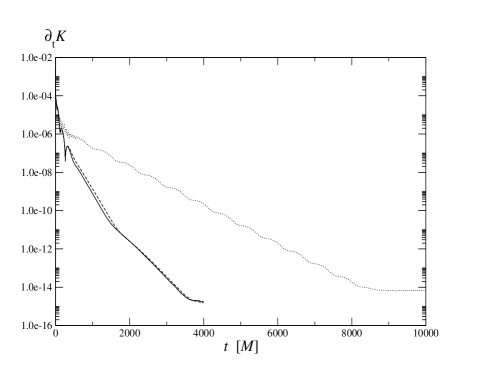
Figure 1: The $\ell_{2}$-norm of the time derivative of $K$ for the evolution of a static iEF black hole in octant symmetry using 1+log slicing expressed in terms of the lapse (solid curve) and densitized lapse (dashed curve). The dotted line is from a simulation using an algebraic densitized lapse

The run represented by the dotted line was intended to address the question of whether such long-term stable evolutions can also be achieved if we use the purely algebraic gauge conditions given by Eq. (3), with $q$ obtained from the exact iEF solution. The answer is affirmative; that is, condition (3) in conjunction with second-order extrapolation on the excision boundary yields qualitatively similar results to those depicted by the solid and dashed lines. The motivation for switching for this run from simple excision to an excision with extrapolation of the grid-functions lies in anticipation of the wobbling black hole simulations. When the evolved black hole solution is time-dependent (as is the case of a wobbling black hole), simple excision is no longer suitable. The copying of time-derivatives at the excision boundary used in simple excision becomes effectively a boundary condition on the spatial derivatives of grid-functions. This boundary condition is incompatible with the outflow nature of the excision boundary.

Comparison of the dotted line with the solid and dashed lines in Fig. 1 shows that the algebraic densitized lapse run possesses long-term stability. The difference is mostly in the variation of the time when machine precision is reached. In summary, using an analytic densitized lapse $q$ or equivalently an algebraic lapse $\alpha$, we are able to evolve a single black hole with stability properties comparable to those obtained with differential conditions such as 1+log slicing and the $\Gamma$-driver condition for the shift vector. While it is not clear how helpful such analytic slicing conditions will be for simulations of a merging binary black hole, the introduction of a densitized lapse makes them at least available for serious consideration in long-term stable simulations carried out with the BSSN scheme.

III.2 Evolutions of single moving black holes

We now turn our attention to single black holes moving across the numerical grid. One way to obtain such a scenario is to evolve a single boosted black hole. The ensuing motion will, however, move the black hole off the computational domain. With the sizes of the computational domain currently restricted by available hardware resources, this will happen on time scales significantly shorter than those considered relevant for black hole orbits or for testing long-term stability of simulations, namely simulations lasting more than $1000M$.

In Paper I, we introduced therefore an alternative approach which facilitates the motion of single black holes with trajectories confined to the computational domain. We transformed the iEF black hole solution to coordinates $\bar{x}^{\alpha}$ such that

$$t = \bar{t},$$ (9)

$$x^{i} = \bar{x}^{i}+\xi^{i}(\bar{t})\,.$$ (10)

In terms of the new coordinates, the line element becomes

$$ds^{2}=-\alpha^{2}d\bar{t}^{2}+\gamma_{ij}\left(d\bar{x}^{i}+\bar{\beta}^{i}\,d\bar{t}\right)\left(d\bar{x}^{j}+\bar{\beta}^{j}\,d\bar{t}\right)\,,$$ (11)

where

$$\bar{\beta}^{i}=\beta^{i}+\dot{\xi}^{i}.$$ (12)

In Paper I, this method was used to move black holes on circular and bouncing trajectories. Using either a cubical or spherical excision region, these runs lasted for about $130\,M$, though the apparent horizon started to intersect the excision region at about $90\,M$ and the apparent horizon finder failed to give reasonable results afterwards. The fixed gauge conditions used in these evolutions were considered a crucial limiting factor in those evolutions.

Using the densitized lapse condition (3) with $n=1$, we performed similar simulations to those in Paper I. We fix the value of $q$ in Eq. (3) from the exact single iEF black hole solution transformed according to Eqs. (10), (12). In Fig. 2, we plot the $\ell_{2}$-norm of the Hamiltonian constraint (upper panel) and normalized Hamiltonian constraint (lower panel) for simulations of a black hole on a circular path with radius $2\,M$ and orbital frequency $1/(2\pi)$. Equatorial symmetry is assumed for all the simulations, and the outer boundary conditions consist of setting the values of the grid-functions to the exact analytic solution.

Fig. 2 depicts results from four simulations. In the upper panel from top to bottom, each data set corresponds to computational domains $20\times 20\times 7\,M^{3}$, $20\times 20\times 10\,M^{3}$, $30\times 30\times 7\,M^{3}$ and $30\times 30\times 10.5\,M^{3}$, respectively. In the lower panel, the correspondence is reversed. That is, from top to bottom at early times, each data set is for domains $30\times 30\times 10.5\,M^{3}$, $30\times 30\times 7\,M^{3}$, $20\times 20\times 10\,M^{3}$ and $20\times 20\times 7\,M^{3}$, respectively. The shortest scale is along the direction perpendicular to the orbital plane.

The results in Fig. 2 from the $20\times 20\times 7\,M^{3}$ run should be compared with Fig. 9 of Paper I where simulations lasted $<130\,M$. This comparison clearly demonstrates the tremendous improvement on the duration of the simulations when a densitized lapse is used. Some of the evolutions are stable at least for $6000\,M$, when the runs were terminated due to limitations of computational resources. Fig. 2 also demonstrates that, even though the durations of the simulations have been improved by at least an order of magnitude, the simulations continue to be affected by boundary effects. This is expected since it is well known that setting boundary conditions to the exact analytic solution is conducive to numerical instabilities.

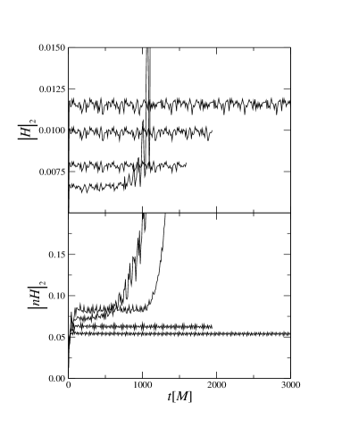
Figure 2: The $\ell_{2}$-norm of the Hamiltonian constraint (upper panel) and normalized Hamiltonian constraint (lower panel) are shown as a function of time for the circling black holes for different sizes of the computational domain. See text for details.

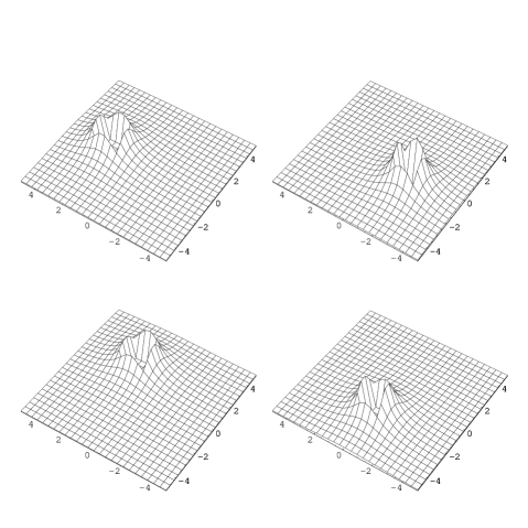
Figure 3: The four panels show snapshots of the evolution of $K$ for a circling black hole in the $xy$-plane at times $0$, $2000\,M$, $4000\,M$ and $6000\,M$.

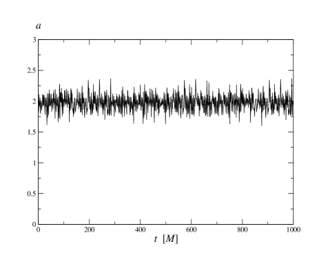
Figure 4: The order of convergence for the circling black hole obtained from evolutions using a resolution of $M/4$ and $M/5$. Second-order convergence is clearly maintained for long times.

In Fig. 3 we show snapshots of the evolution obtained on the domain $20\times 20\times 7\,M^{3}$ at $t=0$, $2000\,M$, $4000\,M$, $6000\,M$. Here we plot the variable $K$ on the $xy$-plane at $z=0$, namely the orbital plane. The excision region is clearly visible and has been checked lie within the apparent horizon. We find the apparent horizon area to remain within a few per cent of its analytic value $16\,\pi\,M^{2}$ and the deviation from spherical shape to be of the same order. The method we have used to enable the excision region to follow the motion of the black hole is based on an analysis of the asymmetry and fall-off behavior of grid variables near the excision region (see next section for details). This method is in general not coordinate invariant and its performance needs to be monitored by verifying that the excision region always remains inside the apparent horizon. We have verified this for all runs discussed in this paper Den .

By construction, our numerical code is second-order accurate. Fig. 4 shows the ability of our code to maintain second-order convergence. Because demonstrating long-term convergence requires considerable computational resources, we have only performed the convergence analysis for times $<1000\,M$. The jaggedness in these plots is due to the requirement that the center of the excision region always be located on a grid point. The excision mask will therefore move across the computational domain in a discontinuous fashion.

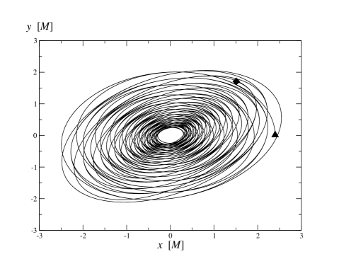
Figure 5: The trajectory of a black hole in-spiraling between radius $2.5$ and $0.25$. The initial position is marked by the filled triangle and the end position by the diamond. The $z$-position will remain zero throughout the evolution.

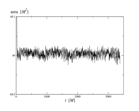
Figure 6: The apparent horizon area for the evolution of a spiraling black hole. The value predicted from the exact analytic solution is $16\,\pi\,M^{2}\simeq 50.27\,M^{2}$

In order to further test the robustness of our excision infrastructure, we have performed the same type of evolution using a different black hole trajectory. Having in mind the eventual target of simulating in-spiraling binary black holes, it will be of particular interest to see whether the code is able to evolve a black hole on an in-spiraling trajectory. We consider such a scenario by fixing the location of the black hole singularity, $\vec{\xi}=(\xi^{1},\xi^{2})$ [cf. Eq. (10)], from the solution of the differential equation

$$\partial_{tt}\vec{\xi}+D\,\partial_{t}\vec{\xi}+\nabla\Phi=0\,,$$ (13)

with $\xi^{3}=0$ because the black hole orbit is confined to the plane $z=0$. The potential is given by $\Phi=C\,[(\xi^{1})^{2}+(\xi^{2})^{2}]$ and $D$ and $C$ are constants.

We emphasize that none of these quantities has any connection to realistic astrophysical simulations. They merely serve to determine the components $\xi^{i}$ in the coordinate transformation (10) and, thus, the artificial black hole trajectory. We obtain an in-spiraling trajectory by choosing $D=C=0.01$. The black hole is initially placed at a distance of $2.4\,M$ from the origin at $z=0$ and given an initial purely tangential velocity $v=0.3$. Because of the damping, the velocity and radius will decrease and the black hole would eventually approach a steady state at the origin. In order to keep the evolution dynamic for long times, we switch the sign of the damping term when the radius shrinks below $0.25\,M$ after which the hole starts spiraling outward. The damping constant is switched back to a positive value once a radius of $2.5\,M$ is reached and so on. The resulting trajectory in the $xy$-plane is displayed in Fig. 5. This path corresponds to an evolution lasting $3500\,M$ when we decided to terminate the evolution.

The apparent horizon finder had no difficulty calculating the outermost trapped surface every $20\,M$. The resulting horizon area is shown as a function of time in Fig. 6. The area remains constant with good accuracy and deviates by a few per cent from the analytic value of $16\pi\,M^{2}$. Similarly we found the error in the Hamiltonian constraint normalized with respect to its individual addends to be constant to within about $6\,\%$.

IV The excision tracking method

For the dynamic evolutions of the previous section, we have used a simple mechanism by which the excision region tracks the movement of the black hole. We will describe this method in more detail now.

In order to make use of the causal disconnection of the black hole interior it is imperative that the excision region be located within the event horizon of the black hole. Because the location of the event horizon requires analysis of the global (in space and time) data and can thus not be carried out during the evolution itself, one commonly resorts to searching for apparent horizons. An apparent horizon (also called a marginally trapped outer surface) is defined locally and can thus be calculated at each time step (see for example Thornburg (1996)). The existence of an apparent horizon guarantees that there is a surrounding event horizon and thus a causal boundary. Ideally one would perform a search for an apparent horizon at each time step and adjust the location of the excision region correspondingly. Unfortunately the calculation of apparent horizons is computationally expensive although recent work by Thornburg Thornburg (2003) seems to overcome some of these difficulties. It appears, nonetheless, desirable to have available a reliable, computationally inexpensive method of dynamically adjusting the location of the excision regions to accommodate the movement of the black holes. One may then calculate the apparent horizon at regular intervals to monitor the causal consistency of the excision procedure.

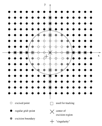
Figure 7: A schematic illustration of the excision region (the $z$-direction is suppressed). The $x$ and $y$-axes in this diagram are coordinate lines through the current excision center ($\times$) whereas the black hole is centered at the $+$. Data at at the points marked by a box are used to analyze the symmetry properties of a grid variable and update the excision center.

For this purpose we have used a simple scheme which analyzes the fall-off and symmetry behavior of evolution variables near the black hole singularity to predict a reasonable value for the central position of the excision region. The excision technique used in our Maya code has been described in detail in Paper I, and we will focus here on those parts added for the tracking of the excision center. In Fig. 7 we have schematically plotted a 2-dimensional slice of a spherical excision region (the precise shape of that region is irrelevant for our method). The current excision center is marked by the symbol $\times$. Assuming that the black hole is slightly offset with respect to this position, we have marked by a $+$ the desirable location of the excision center. In a loose sense we might call this the current black hole position. We note, however, that a precise definition of a black hole center, as for example in terms of a point-like singularity, can only be given for a restricted subclass of black holes.

For concreteness, we now consider analytic data for a static black hole of mass $M=1$ in iEF coordinates located at $x=-0.105$, $y=0$, $z=0$. We describe this data in terms of an excision region with radius $0.7$ centered at $x=0$, $y=0$, $z=0$. Quite obviously this is not the optimal position of the excision region and the data will show some asymmetry in their fall-off behavior in the vicinity of the excision boundary. The idea is then to construct some combination of the field variables which adequately exhibits this behavior. Such a combination will in general not be coordinate-invariant and thus depends on the scenario under investigation. For all runs presented in this paper, we have found the trace of the extrinsic curvature $K$ a perfectly adequate choice. A 1-dimensional plot in Fig. 8 of $K$ along the $x$-axis through the excision center reveals the asymmetry. The $\times$ symbols in this figure correspond to the values of $K$ at the 8 points marked by boxes on the $x$-axis in Fig. 7. At the end of each evolution step in our code we fit a Gaussian

$$a\,e^{\frac{(x-b)^{2}}{c^{2}}}$$ (14)

through these points. The parameters $a$, $b$ and $c$ are obtained from $\chi^{2}$-minimization and the value for $b$ gives us the $x$-coordinate of the updated excision center. We then proceed similarly for the $y$ and $z$ direction. If further excision regions are

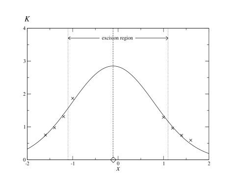
Figure 8: Numerical data ($\times$) on the $x$-axis (cf. Fig. 7) around the excision region is fitted with a Gaussian curve (solid line). The central position of the Gaussian is used as the updated $x$ value of the excision center. The diamond marks the exact location of the singularity used for these data and is well-approximated by the fitting algorithm.

present in the computational domain they are treated in the same way. The total number of points used for this method is a free parameter but we typically find 8 (as in this example) to be sufficient.

With regard to non-stationary scenarios it is, of course, possible that a certain asymmetry of the data might arise from reasons unrelated to the black hole location, as for example in the case of boosted black holes. We emphasize, however, that the purpose of this algorithm is not to provide as accurate as possible an estimate of a black hole center (which in many cases will not be well defined anyway), but to prescribe a recipe for centering the excision region. The only requirement for a healthy evolution is that the excision region be contained entirely within the apparent horizon. This may be monitored, for example, by regular calculations of the apparent horizon. In the numerical evolutions presented above we have used a few buffer zones (layers of grid points inside the apparent horizon which are not excised) and verified that the excision region indeed remains confined to the interior of the apparent horizon.

V Conclusions

We have studied the impact of a densitization of the lapse function on the stability properties of BSSN evolutions using singularity excision. We have demonstrated that the use of a densitized lapse preserves the capability of stably evolving a single Schwarzschild black hole using the simple excision technique in combination with a differential slicing condition of the live 1+log type. These numerical simulations settle down to a configuration that remains constant in time up to machine precision.

We have next considered the evolutions of single static black holes in the case where the slicing condition is a prescribed analytic function of the spacetime coordinates. In such scenarios numerical codes using the BSSN scheme have hitherto exhibited significantly poorer stability properties than those based on hyperbolic formulations. As the use of a densitized lapse (or a generalized version thereof) is a necessary ingredient in the majority of hyperbolic formulations, it has naturally been used in these codes in place of the lapse function itself. We have bridged the gap between hyperbolic and BSSN-like formulations, by evolving a stationary single black hole spacetime using the BSSN formulation in combination with a densitized version of the lapse function. We have thus been able to obtain evolutions lasting many thousands of $M$ in which the time-variations decay to machine precision. To our knowledge this has so far not even been achieved with strictly hyperbolic formulations. Regarding the use of purely analytic gauge conditions for such scenarios, our results indicate that the use of a densitized lapse (i.e.  algebraic as opposed to fixed slicing) has been the key advantage of hyperbolic systems over BSSN-like formulations of Einstein’s equations. It is not clear to what extent algebraic gauge conditions will be beneficial in the simulation of in-spiraling binary black holes, but the results presented here demonstrate how such conditions can also be used for long-term stable evolutions carried out in the framework of the BSSN formulation.

These ideas have also shown advantages in evolving black holes moving across the computational domain. By virtue of time-dependent coordinates, we are able to move single iEF black holes through the computational domain on essentially arbitrary paths. The duration of such evolutions has previously been limited to about $100\,M$. Because the motion of the singularity is prescribed in terms of the gauge conditions, these simulations inevitably used analytic gauge. By reformulating this in terms of the densitized lapse, we were able to extend the lifetime of the runs to at least $1000\,M$. This also demonstrates that the dynamic excision techniques used for our simulations are, in principle, capable of handling long-term stable evolutions of moving black holes. We believe that the ideas presented in this work will be helpful for the development of long-term stable evolutions of black hole collisions.