Geometrical optics analysis of the short-time stability properties of the Einstein evolution equations

Abstract

Many alternative formulations of Einstein’s evolution have lately been examined, in an effort to discover one which yields slow growth of constraint-violating errors. In this paper, rather than directly search for well-behaved formulations, we instead develop analytic tools to discover which formulations are particularly ill-behaved. Specifically, we examine the growth of approximate (geometric-optics) solutions, studied only in the future domain of dependence of the initial data slice (e.g. we study transients). By evaluating the amplification of transients a given formulation will produce, we may therefore eliminate from consideration the most pathological formulations (e.g. those with numerically-unacceptable amplification). This technique has the potential to provide surprisingly tight constraints on the set of formulations one can safely apply. To illustrate the application of these techniques to practical examples, we apply our technique to the 2-parameter family of evolution equations proposed by Kidder, Scheel, and Teukolsky, focusing in particular on flat space (in Rindler coordinates) and Schwarzchild (in Painleve-Gullstrand coordinates).

I Introduction

Recently developed numerical codes offer the possibility of extremely accurate and computationally efficient evolutions of Einstein’s evolution equations in vacuum KST . To take full advantage of these new techniques to perform an unconstrained evolution of initial data and boundary conditions, we must address an unpleasant fact: many choices for evolution equations and and boundary conditions permit ill-behaved, unphysical solutions (e.g. growing, constraint-violating solutions) near physical solutions.

By way of example, when Kidder, Scheel, and Teukolsky (KST) evolved a single static Schwarzchild hole as a test case, they found evidence suggesting that their evolution equations and boundary conditions, when linearized about a Schwarzchild background, admitted growing, constraint-violating eigenmodes KST LSenNorms . These eigenmodes were excited by generic initial data (i.e. roundoff error); grew to significant magnitude; and were directly correlated with the time their code crashed. As this example demonstrates, the existence and growth of ill-behaved solutions limit the length of time a given numerical simulation can be trusted – or even run.

For this reason, some researchers have explored the analytic properties of various formulations of Einstein’s equations LSenNorms paADM paShinkaiReview paWeakHyperbolicBad1 paFR paBSSN paEarlyWorkAddConstraints and boundary conditions bcWellPosed1 bcWellPosed2 bcWellPosed3 bcFrittelli used in numerical relativity, searching for ways to understand and control these undesirable perturbations.

In this paper, we discuss one particular type of undesirable perturbation: short-wavelength, transient wave packets. [For the purposes of this paper, a transient will be any solution defined in the future domain of dependence of the initial data slice. Depending on the boundary conditions, the solution may or may not extend farther in time, outside the future domain of dependence. Inside the future domain of dependence, however, “transient solutions” are manifestly independent of boundary conditions.] Depending on the evolution equations and background spacetime used, these transients can potentially grow significantly (i.e. by a factor of more than $10^{16}$ in amplitude). Under these conditions, even roundoff-level errors in initial data should produce transients that amplify to unit magnitude. Once errors reach unit magnitude, then guided by the KST results discussed above, we expect nonlinear terms in the equations to generically cause these errors to grow even more rapidly, followed shortly thereafter by complete failure of a numerical simulation. In other words, if the formulation and background spacetime permit transients to amplify by $10^{16}$, we expect numerical simulations of these spacetimes to quickly fail.

In this paper we develop conditions which tell us when such dramatic amplification is assured. Specifically, we describe how to compute the amplification of certain transients for a broad class of partial differential equations (first-order symmetric hyperbolic PDEs) that includes many formulations of Einstein’s equations. If this amplification is larger than $10^{16}$, then we know we should not evolve this formulation numerically.

I.1 Outline of remainder of paper

In this paper, we analyze the growth of transients. [Remember, in this paper a transient is any solution defined in the future domain of dependence of the initial data slice.] Rather than study all possible formulations, we limit attention to a class of partial differential equations we can analyze in a coherent, systematic fashion: first-order symmetric hyperbolic systems. Furthermore, because we concern ourselves only with stability and the growth of small errors, we limit attention to linear perturbations upon some background. Finally, to be able to produce concrete predictions, we restrict attention to those transients which satisfy the geometric optics approximation.

In Sec. II we introduce an explicit ray-optics-limit solution to first-order symmetric hyperbolic linear systems – a class which includes, among its other elements, linearizations of certain formulations of Einstein’s equations. We provide explicit ODEs which determine the path (i.e. ray) and amplitude of a geometric-optics solution, in terms of initial data at the starting point of the ray. Then, in Sec. III, we introduce wave packets as solutions which are confined to a small neighborhood of a particular ray. We further define two special classes of wave packet – coherent wave packets and prototyptical coherent wave packetes – which, because of their simple, special structure, are much easier to analyze. Finally, in Sec. IV, we introduce and discuss the technique (energy norms) we will use to characterize the amplitude of wave packets. In particular, we provide an explicit expression [Eq. (20)] for the growth rate of energy of a prototypical coherent wave packet.

To demonstrate explicitly how the techniques of the previous sections can be applied to produce the growth rate of transients, in Sections V and VI (as well as Appendix E) we describe by way of example how our methods can broadly be applied to the two-parameter formulations that Kidder, Scheel, and Teukolsky (KST) have proposed KST . Specifically, Sections V and VI will respectively describe wave packets on flat-space (written in Rindler coordinates) and radially propagating transients on a Schwarzchild-black-hole background (expressed in Painleve-Gullstrand coordinates).

Finally, to demonstrate explicitly how expressions for the growth rate of transients can be used to filter out particularly pathological formulations, in Sections VII and VIII we use the results for the growth rates of transients obtained in Sections V and VI to determine what pairs of KST parameters ($\gamma$ and $\hat{z}$) guarantee significant amplification of some transient propagating on a Rindler and Painleve-Gullstrand background, respectively.

Guide to the reader

While the fundamental ideas behind this paper – the study of wave packets and the use of their growth rates to discover ill-behaved formulations – remains simple, when we attempted to perform practical, accurate computations, we quickly found the simplicity of this idea masked behind large amounts of novel (but necessary) notation. We therefore found it difficult to simultaneously satisfy the casual reader – who wants only a summary of the essential results, and who is still evaluating whether the results and the methods used to obtain them are worthy of further attention – and the critical reader – who needs comprehensive understanding of our methods in order to evaluate, duplicate, and (potentially) extend them. We have chosen to slant the paper towards the towards the critical reader; thus this paper is a comprehensive and pedagogical introduction to our techniques.

While this paper can be consumed in a single reading, for the reader interested in a brief summary of the essential ideas and results, or for anyone making a first reading of this paper, the author recommends only reading the most essential details. First and foremost, the reader should understand the scope and significance of this paper (i.e. read the abstract and Sec. I). Next, the reader should follow the general description of the techiques in Sections II, III, and IV in detail. Subsequently, the reader should examine our demonstration that our techniques indeed give correct results for growth rates (cf. the introduction to Section V and the summary that section’s results in Section V.4). Finally, to understand how these techniques can be used to discrover ill-behaved formulations, the reader should examine Sections VII and VIII.

The more critical reader may wish to test and verify our computations. This reader should then review Sections II, III, and IV again, then work through Sections V and VI in detail (returning to the earlier sections for reference as necessary). This reader will also benefit from the general approach to KST 2-parameter formulations discussed in Appendix E.

Finally, the most skeptical readers will want to examine the conceptual underpinnings of and justifications for our every computation. This reader should simply follow the text as presented, but carefully read every footnote and appendix as they are mentioned in the text. In particular, this reader will want to review our Appendicies B (for a justification of our ray-optics techniques) and A (for many useful identities used in the previous appendix and elsewhere in the paper) as well as Appendix C (for a more detailed discussion of prototypical coherent wave packets, a key element in our computational method).

I.2 Connection with prior work

I.2.1 Study a short-time, rather than long time, instability mechanism

First and foremost, we should emphasize that our work differs substantially from all previoius work on this subject: we very explicitly restrict attention to amplification over only a short time (i.e. a light-crossing time). On the one hand, unlike other work, because of this restriction, our claims – being independent of boundary conditions – apply to all boundary conditions. On the other, because we forbid ourselves from studying our solutions outside the future domain of dependence of the initial data slice – even though, in practice, we could draw some elementary conclusions – in this paper we choose not to make any claims about how a formulation of Einstein’s equations will behave at late times (i.e. its late-time stability properties).

I.2.2 Study an instability mechanism, not necessarily the dominant one

In other papers which attempt to address the stability properties of various formulations of Einstein’s equations – for example, Lindblom and Scheel (LS) LSenNorms – the authors try to (somewhat naturally) an understanding of the dominant instability mechanism. Unfortunately, we do not fully understand all the dominant instability mechanisms which can occur in generic combinations of evolution equations, boundary conditions, and background spacetimes. Indeed, while some theoretical progress has been made towards estimating the dominant instability mechanisms (i.e. LS), for generic “reasonable” formulations (i.e. those which we have not excluded based on other known pathologies, such as being weakly hyperbolic), we currently can only reliably determine how effective simulations will be by running those simulations. And simulations are slow.

In this paper, instead of studying the dominant instability, we study an instability (transients) which we can easily understand and rigorously describe. We use this instability to discover formulations which are known to be troublesome (i.e. which have trouble with transients).

I.2.3 Short-wavelength approximations

This paper makes extensive use of geometric optics, a special class of short-wavelength approximation. Several authors have applied short wavelength techniques to study the stability of various formulations of Einstein’s equations paADM , paShinkaiReview , paFR . These techniques, however, have generally been applied to systems whose coefficients do not vary in space, limiting their validity either to very small neighborhoods of generic spacetimes, or to flat space. Previous analyzes have thus obtained only a description of local plane wave propagation: in other words, local dispersion relations. In this paper, with the geometric optics approximation, we describe how to glue these local solutions together. Such gluing is essential if we are to obtain a good approximation to a global solution of the PDE and hence a concrete, reliable estimate of the amplification of a transient. In this sense, the present paper is the logical extension of work by Shinkai and Yoneda (see, e.g., paShinkaiReview ), an attempt at converting their analysis to precise, specific conditions one can impose which insure that transients do not amplify.

I.2.4 Energy norms

This paper also employs the energy-norm techniques introduced by Lindblom and Scheel (LS) LSenNorms . Energy norms provide a completely generic approach to determining the growth rate given a known solution and, moreover, can be used to bound the growth of generic solutions. While LS choose to apply these techniques to study a different class of solution – large-scale solutions whose growth presently limits their numerical simulations – these techniques remain generally applicable. We use them to characterize the growth of wave packets.

II Ray optics limit of first-order symmetric hyperbolic systems

In classical electromagnetism, certain short-wavelength solutions to Maxwell’s equations can be approximated by a set of ordinary differential equations for independently-propagating rays: a set of equations for the path a ray follows, and a set of equations which determine how the solution evolves along a given ray BornWolf . This limit is known as the ray optics (or geometric-optics) limit. In this section, we construct an analogous limit for arbitrary first-order symmetric hyperbolic linear systems.

II.1 Definitions

We study a specific region of 4-dimensional coordinate space ($t,\vec{x}$), on which at each point we have a $N$-dimensional (real) vector space $V$ of “fields” $u\in V$.

Inner products: On the space of fields, an inner product is a map from two vectors $u,v$ to a real number with certain properties (bilinear, symmetric, and positive-definite). The inner product is assumed to be smooth relative to the underlying 4-manifold. The canonical inner product on $R^{N}$ (i.e. the $N$-dimensional dot-product, relative to some basis of fields which is defined everywhere throughout space) is denoted $(,)$, and does not vary with space. We can represent any other inner product in terms of the canonical inner product and a map $S:V\rightarrow V$ as $(u,Sv)$, where $(u,Sv)=(Su,v)$.

An operator $Q$ is said to be symmetric relative to the inner product generated by $S$ if $(u,SQv)=(Qu,Sv)$ for all $u,v$. In other words, an operator $Q$ is symmetric if it is equal to its own conjugate relative to $S$, denoted $Q^{\dagger}$ and defined by $(u,SQv)=(Q^{\dagger}u,Sv)$ for all $u,v$. Equivalently, the conjugate $Q^{\dagger}$ relative to $S$ may be defined in terms of the transpose $Q^{T}$ (i.e. the conjugate relative to $S=1$):

$$Q^{\dagger}\equiv S^{-1}Q^{T}S\;.$$ (1)

First-order symmetric hyperbolic linear systems (FOSHLS): A first-order symmetric hyperbolic linear system has the form

$$\left[\partial_{t}+A^{a}(x,t)\partial_{a}-F(x,t)\right]u(\vec{x},t)=0$$ (2)

for $u(x,t)$ a smooth function from the underlying 4-manifold into the $N$-dimensional space of fields, for $A^{a}$ and $F$ some (generally space and time dependent) linear operators on that space, and for $A^{a}$ a symmetric operator relative to some inner product.

If more than one inner product makes $A$ symmetric, henceforth, when talking about a specific FOSHLS, we shall fix one specific (arbitrary) inner product throughout the discussion, and therefore some specific $S$.

Characteristic fields and speeds: For all 3-vectors $p_{a}$, $A^{a}p_{a}$ is symmetric relative to the inner product generated by $S$. It has a set of eigenvalues, eigenspaces, and (for each eigenspace) basis eigenvectors, denoted as follows:

• $\omega_{j}(t,\vec{x},\vec{p})$ are the eigenvalues of $A^{a}p_{a}$;

• $B_{j}(t,x,p)$, where $j$ runs from 1 to the number of distinct eigenvalues of $A^{a}p_{a}$, are the eigenspaces of $A^{a}p_{a}$; and

• $v_{j,\alpha}(t,\vec{x},\vec{p})$ are some orthonormal basis of eigenvectors for the space $B_{j}(t,x,p)$, where $\alpha$ runs from 1 to the dimension of $B_{j}$.

Because $A^{a}p_{a}$ is symmetric relative to the inner product induced by $S$, the eigenspaces are orthogonal relative to the inner product, and the eigenspaces are complete. Finally, at each point $(x,p)$ and for each eigenspace, there is a unique projection operator $P_{j}(t,x,p)$ which satisfies $P_{j}v=v$ if $v\in B_{j}$, $P_{j}v=0$ if $v\in B_{k}$ with $k\neq j$.

We require $A^{a}p_{a}$ and its eigenvalues, eigenspaces, and projection operators to vary smoothly over all $x^{a}$ and $p_{b}$ in the domain. [We do not demand the eigenvectors themselves to be smooth save in the neighborhood of each point $(x^{a},p_{b})$: topological constraints may prevent one from defining an eigenvector everywhere (i.e. for all $p_{a}$ given $x^{a}$) .]

Group velocity and acceleration: We define the group velocity $V_{j}^{a}$ and group acceleration $a_{j,a}$ via

$$V_{j}^{a}(t,\vec{x},\vec{p}) \equiv \frac{\partial}{\partial p_{a}}\omega_{j}(t,\vec{x},\vec{p})\;,$$ (3)

$$a_{j,a}(t,\vec{x},\vec{p}) \equiv -\frac{\partial}{\partial x^{a}}\omega_{j}(t,\vec{x},\vec{p})\;.$$ (4)

We shall make frequent use of an alternative expression for the group velocity, Eq. (60), which is discussed in Appendix A. Among other things, Eq. (60) implies

$$\omega_{j}(x,p)=V^{a}_{j}p_{a}\;.$$

II.2 Form of ray-optics solution

We now construct a solution which approximately satisfies Eq. (2). Our method works by constructing a set of characteristics (i.e. rays), then integrating some amplitude equations along each characteristic (as an ODE) to find the amplitudes farther along the ray.

In this section, we only introduce the results of our analysis. In Appendix B, we provide a more comprehensive justification of our ray-optics approach.

Ray-optics solution

Rather than express our solution in terms of the original $N$-dimensional variable $u$, we introduce $N+1$ new variables $d_{j,\alpha}$ and $\phi$ and parametrize the original state by

$$u=\bar{u}e^{i\phi}$$ (5)

where we further expand $\bar{u}$ in terms of the eigenvectors $v_{l,\alpha}$ of $A^{a}\partial_{a}\phi$ at each point $(t,\vec{x})$:

$$\bar{u}=\sum_{l}\sum_{\alpha}d_{l,\alpha}(t,x,\partial\phi)v_{l,\alpha}\left(t,x,\partial\phi\right)\;.$$ (6)

[For notational clarity, the arguments $t$, $\vec{x}$, and $\partial_{a}\phi$ to the functions $\phi$, $v_{l,\alpha}$, and $d_{l\alpha}$ will in the following be usually omitted.]

In terms of these new variables, a ray-optics solution is a solution to the following equations, for some fixed $j$:

$$0 = \left[\partial_{t}+V_{j}^{a}(x,\partial\phi)\partial_{a}\right]\phi\;,$$ (7a)

$$0 = d_{l,\beta}\quad\text{for}\;l\neq j\;,\text{ and}$$ (7b)

$$0 = \left[\partial_{t}+V_{j}^{a}\partial_{a}\right]d_{j,\alpha}$$

$$+\sum_{\beta}d_{j,\beta}\bigg{(}v_{j,\alpha},\;S(\partial_{t}+A^{a}\partial_{a}-F)v_{j,\beta}\bigg{)}\;.$$

When we substitute solutions to the ray-optics equations [Eq. (7)] back into the original FOSHLS [Eq. (2)], as described in detail in Appendix B, we find the geometric-optics solutions are excellent approximate solutions to the original PDE, so long as certain mild conditions continue to hold [e.g. the oscillations in $\phi$ remain rapid compared to any other length or time scale].

II.3 Interpreting the geometric-optics equations

We introduce the geometric-optics solution precisely because it simplifies the PDE – in particular, because it converts the problem of solving a general PDE [Eq. (2)] into the problem of solving uncoupled ODEs [Eq. (7)]. Specifically, these ODEs consist of the the phase equation [Eq. (7a)] – which determines the path of the ray leaving a point $\vec{x}$ consistent with initial data for $\phi$ with gradient $\partial_{a}\phi(\vec{x})$ – and the polarization equations [Eqs. (7b) and (7)] – which allow us to propagate the $d_{l,\alpha}$ along each ray.

But while these equations are now ODEs, their structure is not particularly transparent. In this section, we rewrite the phase equation [Eq. (7a)] and the polarization equation [Eq. (7)] to better emphasize their properties and physical interpretation.

II.3.1 Path of the ray

The physical significance of the phase equation [Eq. (7a)] becomes much easier to appreciate when it is rewritten in first-order form. When we differentiate that expression and re-express the result as an equation for $k_{a}\equiv\partial_{a}\phi$, we find

$$0 = \partial_{t}k_{a}+V_{j}^{b}\partial_{b}k_{a}+[\partial_{a}V_{j}^{b}(x,k)]k_{b}$$ (8)

$$= \partial_{t}k_{a}+V_{j}^{b}\partial_{b}k_{a}-a_{j,a}(x,k)\;.$$

[While $k$ does depend on $x$, because $(\partial_{k_{c}}V_{j}^{b})k_{b}=0$ the last term in the first line does indeed simplify into $-a_{j,a}$, as stated]. Solutions to this PDE may be constructed by gluing together solutions to the following pair of coupled ODEs for $\vec{x}(t)$ and $\vec{k}(t)$:

$$\frac{dx^{a}}{dt} = V^{a}_{j}(\vec{x},\vec{k})$$ (9a)

$$\frac{dk_{a}}{dt} = a_{a,j}(\vec{x},\vec{k})\;.$$ (9b)

By using the definitions of $V^{a}_{j}$ and $a_{a,j}$, we find these are precisely Hamilton’s equations, using $\omega_{j}(t,x,k)$ as the Hamiltonian.

These two equations define the rays (i.e. characteristics). Given initial data for $k_{a}$ which has $k_{a}=\partial_{a}\phi$ in a 3-dimensional neighborhood of a point, we have a unique ray emanating from each point in that neighborhood. Solutions to Eq. (8) follow from joining the resulting rays emanating from each point in the neighborhood together; and solutions for $\phi$ [i.e. Eq. (7a)] follow by integrating the phase out along each ray.

II.3.2 Propagating polarization along ray

In practice, the polarization equation [Eq. (7)] is difficult to interpret: since it involves spatial derivatives of basis vectors, and since we have freedom to choose our basis vectors $v_{j,\alpha}$ arbitrarily within each subspace $B_{j}$, we cannot transparently disentangle meaningful terms from convention-induced effects.

To constrain the basis and simplify the equation, we sometimes choose a basis in the neighborhood of the ray of interest which satisfies the no-rotation condition [discussed at greater length in Appendix A.2]:

$$\left(v_{j,[{\alpha}},S(\partial_{t}+A^{a}\partial_{a})v_{j,{\beta}]}\right)=0\;.$$ (10)

where the square brackets denote antisymmetrization over $\alpha$ and $\beta$ [i.e. $X_{[\alpha\beta]}=(X_{\alpha\beta}-X_{\beta\alpha})/2$]. The no-rotation condition completely constrains the antisymmetric part of an operator [i.e. the left side of Eq. (10)]; the condition that the basis vectors $v_{j,\alpha}$ remain orthogonal constrains that operator’s symmetric part; and therefore the basis $v_{j,\alpha}$ is necessarily completely specified at any point along a ray in terms of initial data for the basis.

Using the no-rotation condition, we find the polarization equation becomes the less-arbitrary expression [Appendix A.3]:

$$0 = \left(\partial_{t}+V_{j}^{a}\partial_{a}+\frac{1}{2}\partial_{a}V^{a}_{j}(x,\partial\phi)\right)d_{j,\alpha}$$

$$-\sum_{\beta}\left(v_{j,\alpha},\left[SF+\frac{1}{2}\partial_{t}S+\frac{1}{2}\partial_{a}(SA^{a})\right]v_{j,\beta}\right)d_{j,\beta}$$

where in the above $v_{j,\alpha}$ is a no-rotation basis. In Sec. III we will use this expression to motivate the definition of prototypical coherent wave packets, which have an exceedingly simple growth rate.

II.4 When do geometric-optics solutions exist?

Given initial data (say, for $k_{a}$ and $d_{j,\alpha}$ on some initial compact region), we can in practice always find a solution to the geometric-optics equations [Eq. (7)] valid for some small interval $\delta t$ (i.e. by using general PDE existence theorems, like Cauchy-Kowaleski). However, for general initial data we cannot solve the phase equation [Eq. (7a)] for an arbitrary time $T$. By way of example, even if we find each individual ray [i.e. each solution to Eq. (9) emanating from each initial-data point] emanating from our initial data region out to time $T$, these rays may cross before time $T$, rendering the geometric-optics solution for $d_{j,\alpha}$ both singular and inconsistent at the ray-crossing point. (A similar problem arises in classical geometric optics.) Furthermore, depending on the structure of $A^{a}$, certain rays may not even admit extension to time $T$ (i.e. certain rays may be be future-inextendible, precisely like rays striking singularities in GR).

A proper treatment of these technical complications is considerably beyond the scope of this paper. In practice, we will assume we have chosen initial data so that our geometric-optics solution can be evolved to any time $T$, unless it involves transport into a manifest singularity (i.e. a singularity of the spacetime used to generate the FOSHLS) before time $T$. Furthermore, we will assume the solution is well-behaved – that is, the congruence has finite values for $k_{a}$, $V^{a}_{j}$, $a_{a,j}$ and their first derivatives. With a well-behaved solution to the phase equation [Eq. (7a)], we may always find a finite, consistent solution to the polarization equation [Eq. (7)] in terms of the initial data.

III Defining wave packets

In Sec. II, we have constructed approximate solutions to linearized first-order symmetric hyperbolic PDEs in the geometric optics limit. These solutions are constructed by integrating ODEs for (and along) rays [Eq. 7]. Since each ray evolves independently, we are naturally led to consider wave packets – that is, ray-optics solutions which are nonzero only in a (4-d) neighborhood of some (4-space) ray.

In this section, we outline how wave packets may be generally constructed. We also describe the two special classes of wave packets, coherent wave packets and prototypical coherent wave packets (PCWP), which will be the focus of discussion henceforth.

III.1 Constructing wave packets

A wave packet that persists for a time $T$ is some solution to the geometric-optics equations [Eq. (7)] which is nonzero only in some small neighborhood of a ray (i.e. nonzero only within some coordinate length $\delta$ from the central ray).

From a constructive standpoint, while we can easily construct solutions from initial data for $k_{a}$ and $d_{j\alpha}$, we have no transparent way, besides solving the equations themselves, to determine whether a particular set of initial data for $k_{a}$ even generates a congruence which exists and remains well-behaved (e.g. $\partial^{a}V_{b}$ and $\partial_{a}k_{b}$ both finite) for time $T$, let alone whether the specific combination of initial data for $k_{a}$ and $d_{j\alpha}$ yields a geometric-optics solution with support only within a given distance $\delta$ from a ray.

Still, physically we expect we can avoid these technical complications. For example, we expect that, for all rays of physical interest, we can extend the central ray of interest to time $T$ (i.e. characteristics of physical interest can be extended as long as physically necessary). We expect that singular congruences $k_{a}$ can be avoided by proper choice of initial $k_{a}$ data (e.g. the ray equations do not require all congruences near the ray of interest to diverge or come to a focus). And given a well-behaved congruence, we expect we can always choose initial data for $d_{j\alpha}$ in a sufficiently small neighborhood so the solution for $d_{j,\alpha}$ is nonzero only within some fixed distance $\delta$ from the central ray.

Thus, as a proper treatment of these technical complications is considerably beyond the scope of this paper, we shall henceforth simply assume that a wave packet solution can always be constructed about any ray of physical interest.

III.2 Specialized wave packets I: Coherent wave packets

Since rays propagate independently, one can choose arbitrary initial data, and in particular arbitrary polarization directions $w$, and still obtain a wave-packet solution. Here, $w$ is defined by

$$w\equiv\bar{u}/|\bar{u}|\qquad|\bar{u}|\equiv[(\bar{u},S\bar{u})]^{1/2}\;.$$ (12)

We prefer to further restrict attention to those wave packets which have a single, dominant polarization direction $w$ present initially (and therefore for all time). In other words, we require $w$ vary slowly across the wave packet’s spatial extent. Wave packets with this property we denote coherent wave packets.

III.3 Specialized wave packets II: Prototypical coherent wave packets (PCWPs)

While coherent wave packets have a simple polarization structure, characterized by some polarization direction $w$, this polarization structure need not necessarily have a transparent relationship to the terms present in the polarization equation [Eq. (7); or equivalently Eq. (II.3.2) if we use a no-rotation basis]. Therefore, we define prototypical coherent wave packets (PCWPs) as wave packets which have at each time their polarization direction $w$ equal to one of the eigenvectors $f_{j}^{(\mu)}$ of the operator $O_{j}$:

$$O_{j} \equiv P_{j}\left\{F+\frac{1}{2}S^{-1}\left[\partial_{t}S+\partial_{a}(SA^{a})\right]\right\}P_{j}$$ (13)

$$O_{j}f_{j}^{(\mu)} \equiv o_{j\mu}f_{j}^{(\mu)}$$ (14)

where $\mu$, running from $1$ to the dimension of $B_{j}$, indexes the eigenvectors of $O_{j}$. For simplicity, we assume $O_{j}$ has a complete set of eigenvectors.

If PCWPs exist, we expect – because of their relationship to the terms of the polarization equation [Eq. (II.3.2)] – the propagation of their polarization will be much easier to understand. Most notably, as we will show in the next section [Sec. IV], prototypical coherent wave packets have particularly simple expressions for their growth rates [i.e. Eq. (20)].

PCWPs will exist as exact solutions to the polarization equation [Eq. (II.3.2)] only in certain special circumstances; for example, most of the polarizations to be discussed in Sections V and VI admit exact PCWP solutions. However, as demonstrated in more detail in Appendix C, we do not expect the polarization equation to generically admit PCWP solutions.

Nonetheless, as discussed in greater detail in Appendix C, a PCWP with $w=f_{j}^{(\nu)}$ is a good approximate solution to the polarization equation when the eigenvalue $o_{j\nu}$ of $O_{j}$ is sufficiently large. Indeed, by rewriting the polarization equation in the basis $f_{j}^{(\mu)}$, we can show generic coherent wave packets will rapidly converge to a PCWP with $w=f_{s}^{(\nu_{o})}$ for $\nu_{o}$ indexing the eigenvalue of $O_{j}$ with largest real part. In other words, based on Eq. (20), when coherent wave packets grow quickly, they can always be well-described by a PCWP.

IV Describing and bounding the growth rate of wave packets

Since a wave packet is narrow and we care little about its precise spatial extent, we commonly characterize the wave packet by a single number (e.g. a peak amplitude) rather than a generic distribution of polarization over space. Unfortunately, the maximum value of the amplitudes $d_{j,\alpha}$ depend on the spatial extent of the wave packet – in other words, it depends on our choice of congruence, rather than the central ray itself.

Because the amplitude function is subject to focusing effects (through the term $\partial_{a}V^{a}$), we choose to describe the magnitude of the wave packet by the magnitude of its energy norm. Introduced by Lindblom and Scheel (LS), the energy norm is an integral quantity analogous to energy LSenNorms ; and, like the energy of a wave packet solution to Maxwell’s equations, the energy norm will not be susceptible to focusing effects.

In this section, we describe how energy norms can be used to characterize the magnitude of wave packets. We also obtain special expressions for the growth rates of coherent wave packets [Eq. (19)] generally and prototypical coherent wave packets [Eq. (20)] in particular.

Also, for completeness, in Appendix D we provide an explicit, rigorous bound for the growth rate of energy which will not be otherwise used in the paper.

IV.1 Energy norms and the magnitude of geometric-optics solutions

Lindblom and Scheel define the energy norm by way of two quadratic functionals of a solution $u$ [LS Eqs. (2.3) and (2.8)]. When expressed in terms of our notation, these functionals are terms of our notation are

$$\epsilon \equiv (u^{*},Su)\qquad E\equiv\int\mu d^{3}x\;\epsilon\;.$$ (15)

Unlike LS, we do not generically have a preferred spatial metric; we therefore replace the factor $\sqrt{g}$ present in LS Eq. (2.8) by the more generic $\mu$.

We may substitute in the expressions appropriate to a ray-optics solution to obtain excellent approximations to the energy. By way of example, the energy $E_{j}$ of a geometric-optics solution propagating in the $j$th polarization may be expressed as

$$E_{j} \approx \int\mu d^{3}x\;\sum_{\alpha,\beta}d_{j,\alpha}^{*}d_{j,\beta}\left(v_{j,\alpha}^{*},\;Sv_{j,\beta}\right)$$

$$= \int\mu d^{3}x\;\sum_{\alpha}|d_{j,\alpha}|^{2}$$

where the terms neglected are small in the geometric optics limit and where the second line holds because by construction the basis $v_{j,\alpha}$ is orthonormal.

IV.2 Energy norms and the growth rate of wave packets

Following the techniques of Lindblom and Scheel, we can use energy norms and conservation-law techniques to obtain a general expression for the growth rate of a wave packet.

To follow their program, we must generate a conservation law. Define, therefore, an energy current $j^{a}$ [i.e. LS Eq. (2.4)]

$$j^{a} \equiv (u^{*},SA^{a}u)\;.$$

The quantities $\epsilon$ and $j^{a}$ obey the conservation-law-form equation

$$\partial_{t}\epsilon+\mu^{-1}\partial_{a}\left(\mu j^{a}\right)=(u^{*},SF{u})+(F{u}^{*},S{u})$$

$$+\left({u},\left[\partial_{t}S+\mu^{-1}\partial_{a}\left(\mu SA^{a}\right)\right]{u}\right)\;$$

[i.e. the analogue of LS Eqs. (2.5) and (2.6)].

For a wave-packet solution, which is concentrated at each time to a small spatial region, the current $j^{a}$ drops to zero rapidly, and is in particular zero at the manifold boundary. As a result, when we integrate the conservation law, we find the energy obeys the equation

$$\frac{dE}{dt} = \int\mu d^{3}x\left({u}^{*},SQu\right)$$ (17a)

$$Q \equiv F+S^{-1}\left[F^{T}S+\partial_{t}S+\mu^{-1}\partial_{a}(\mu SA^{a})\right]$$ (17b)

where $F^{T}$ is defined so $(u,Fv)=(F^{T}u,v)$ for all $u$, $v$ (i.e. $F^{T}$ is the transpose). [In LS, the analogous equations are (2.7) and (2.9); in our case, however, we have no surface term involving $j_{a}$ because the solution falls off rapidly away from the wave packet.]

We can show $Q$ is symmetric relative to $S$. We can also show that that $Q$ is closely related to the symmetric part of the operator $O_{j}$ [Eq. (13)]:

$$P_{j}QP_{j}=O_{j}+O_{j}^{\dagger}+\frac{\partial_{a}\mu}{\mu}P_{j}V_{j}^{a}\;.$$ (18)

IV.3 Energy norms and the growth rate of coherent wave packets

Since coherent wave packets are both localized and possess a well-defined polarization direction $w$, we find Eq. (17) becomes, for coherent wave packets,

$$\frac{1}{E}\frac{dE}{dt} \approx \left({w}^{*},SQ{w}\right)$$ (19)

where the right side is evaluated at the location of the wave packet at the current instant.

Because we still need the appropriate polarization direction $w$ to make use of the above expression – a direction we can only obtain from the polarization equation [Eq. (II.3.2)] – Eq. (19) provides only an alternate perspective on the growth of wave packets, not an entirely independent approach to the evolution of the amplitude.

IV.4 Energy norms and the growth rate of PCWPs

In the special case of a PCWP, however, we do know the polarization direction $w$: it is one of the normalized eigenvectors $f_{j}^{(\mu)}$ of the operator $O_{j}$ [see Sec. III.3]. In this case, we find the energy growth rate for a PCWP with $w=f_{j}^{(\mu)}$ to be

$$\frac{1}{E_{j\mu}}\frac{dE_{j\mu}}{dt}=o_{j\mu}+o_{j\mu}^{*}+\frac{\partial_{a}\mu}{\mu}V_{j}^{a}\;.$$ (20)

[Here, we used Eq. (18) in Eq. (19).]

V Geometric optics limit of KST: Rindler

In the previous sections (Sections II, III, and IV), we have developed a procedure for computing the evolution and amplification of ray-optics solutions in general and prototypical coherent wave packet solutions in particular. To provide a specific demonstration of these methods, we demonstrate how to construct the geometric optics limit (as described in Section II) and compute the growth rate of wave packets (as described in Sections III and IV) when the first-order hyperbolic system is the 2-parameter first-order symmetric hyperbolic system Kidder, Scheel, and Teukolsky introduced (see their Section II J), linearized about a flat-space background in Rindler coordinates.

Our computations in this section proceed as follows. First, we review Rindler coordinates and the effects of using Rindler coordinates as the background in the linearized KST equations. We then describe the limited set of rays we will study (i.e. rays that propagate only in the $x$ direction). Subsequently, we construct the explicit form of the polarization equation [Eq. (7)] for packets that propagate only in $x$. [The analysis simplifies substantially because the basis vectors used do not vary with $x$; therefore, the derivatives present in Eq. (7) disappear.] The analysis of the polarization equation leads us directly to an an explicit expression for the growth of energy of a coherent wave packet [Eq. (17)] in general and a prototypical coherent wave packet in particular [Eq. (20)].

Finally, to verify our expressions give an accurate description of the growth of PCWPs, we compare them them against the results of numerical simulations.

V.1 Generating the FOSHLS using the background Rindler space

Flat space in Rindler coordinates is characterized by the metric

$$ds^{2}=-x^{2}dt^{2}+(dx^{2}+dy^{2}+dz^{2})\;,$$ (21)

for $x>0$. Using this spacetime as a background, we can linearize the KST 2-parameter formulation to generate a FOSHLS of the form of Eq. (2) – and in particular find explicit forms for the operators $A^{a}$ and $F$. For example, we find that the principal part has the form [KST Eq. (2.59), along with the definition of $\hat{\partial}_{o}$ in KST Eq. (2.10)]:

$$\partial_{t}\delta g_{ij} \simeq 0$$ (22a)

$$\partial_{t}\delta P_{ij}+xg^{ab}\partial_{a}\delta M_{bij} \simeq 0$$ (22b)

$$\partial_{t}\delta M_{kij}+x\partial_{k}\delta P_{ij} \simeq 0$$ (22c)

As the right-hand sides of these equations are very long, we shall not provide them, or an explicit form for $F$, in this paper.

Using the FOSHLS obtained by linearizing, we can proceed generally with any linear analysis, including a construction of the geometric-optics limit.

V.2 Describing local plane waves by diagonalizing $A^{a}\hat{x}_{a}$

The geometric-optics limit is a short-wavelength limit. Naturally, then, the first step towards the geometric-optics limit is understanding the plane-wave solutions in the neighborhood of a point. We find these solutions by substituting into Eq. (2) the form $u\propto u_{o}\exp i(k\cdot x-\omega t)$; assuming $k$ and $\omega$ are large, so we may disregard the right side; assuming both $u_{o}$ and $A^{a}$ are locally constant; and then solving for $u_{o}$ and the relationship between $k_{a}$ and $\omega$. In other words, we find those local-plane-wave solutions by diagonalizing $A^{a}k_{a}$, as discussed in Sec. II, to find eigenvalues $\omega_{j}$ and eigenvectors $v_{j,\alpha}$, where $j$ indexes the resulting eigenvalues and $\alpha$ indexes the degenerate eigenvectors for each $j$.

Because the principal part is both simple and independent of the two KST parameters ($\hat{z}$ and $\gamma$), we can diagonalize it by inspection. For every propagation direction, the eigenvalues are precisely $\omega_{s}(x,k)=s|k|$ for $s=\pm 1,0$. For our purposes, we study only propagation in the $x$ direction. Thus, we need only the eigenfields of $A^{a}\hat{x}_{a}$, which are [see KST Eq. (2.61) and also Appendix E.1.3]

$$U^{g}_{ab} = g_{ab}$$ (23a)

$$U^{0}_{y,ab} = M_{yab}$$ (23b)

$$U^{0}_{z,ab} = M_{zab}$$ (23c)

$$U^{\pm}_{ab} = \frac{1}{\sqrt{2}}\left(P_{ab}\pm M_{xab}\right)$$ (23d)

These expressions may be interpreted as equivalent to the basis vectors $v_{j,\alpha}$, as discussed in Appendix E [see Appendix E.1.3, and in particular Eq. (83)].

V.3 Deriving the polarization and energy equations, for propagation in the $x$ direction on the light cone

In this section, we describe how to construct and analyze the polarization equation [Eq. (7)] and energy equation [Eq. (17)] for wave packets propagating in the $x$ direction. For technical convenience, we limit attention to rays which propagate on the light cone – in other words, which travel on one of the two null curves of the metric:

$$dx/dt=sx$$

for $s=\pm 1$.

V.3.1 Essential tool: Diagonalizing $P_{s}FP_{s}$

We have the polarization equation [Eq. (7)] and a basis [Eq. (23), or equivalently Eq. (83)]; the application is straightforward. We can, however, substantially simplify our expression by changing the basis used to expand $\bar{u}$ from $v_{j,\alpha}$ to the basis of eigenvectors $f_{s}^{(\mu)}$ of $P_{s}FP_{s}$, defined by the normalized solutions to

$$Ff_{s}^{(\mu)}=\zeta_{s,\mu}f_{s}^{(\mu)}\;.$$

[Equivalently, we may define these eigenvectors in component fashion. For each $s$, the matrix $(v_{s,\alpha},Fv_{s,\beta})$ admits a complete set of normalized eigenvectors $f_{s,\alpha}^{(\mu)}$:

$$\sum_{\beta}(v_{s,\alpha},Fv_{s,\beta})f_{s,\beta}^{(\mu)}=\zeta_{s,\mu}f_{s,\alpha}^{(\mu)}\;.$$

Using these eigenvectors, we regenerate $f_{s}^{(\mu)}=\sum_{\alpha}f_{s,\alpha}^{(\mu)}v_{s,\alpha}$, which are eigenvalues of $P_{s}FP_{s}$.]

These eigenvectors may be classified according to their symmetry properties under rotations about the propagation axis $x$:

• Symmetric-traceless-transverse 2-tensor [basis vectors correspond to the fields $U^{s}_{yz}$ and $(U^{s}_{yy}-U^{s}_{zz})/\sqrt{2}$] One subspace corresponds to the 2-dimensional space of symmetric-traceless 2-dimensional tensors transverse to the propagation direction. The operator $P_{s}FP_{s}$ is degenerate in this subspace; the single eigenvalue associated with this subspace is given by $\zeta_{s,t}$, defined by

  $$\zeta_{s,t}=-s$$ (24a)

• Transverse 2-vector [basis vectors correspond to the fields $U^{s}_{xz}$ and $U^{s}_{xy}$] Another subspace corresponds to the 2-dimensional space of 2-dimensional vectors transverse to the propagation direction. Again, the operator is degenerate on this space. The eigenvalue of $F$ in this subspace is given by $\zeta_{s,v}$ for

  $$\zeta_{s,v}=-s\frac{1+\gamma}{-1+2\gamma}$$ (24b)

• 2-scalars [spanned by vectors corresponding to the fields $U^{s}_{xx}$ and $(U^{s}_{yy}+U^{s}_{zz})$] Finally, the 2-dimensional space of rotational 2-scalars has its degeneracy broken by $F$. For each $s$, we find two eigenvalues, denoted $\zeta_{s,s1}$ and $\zeta_{s,s2}$, with values

  $$\zeta_{s,s1} = -s$$ (24c)

  $$\zeta_{s,s2} = -s\frac{1+2\gamma^{2}}{-1+2\gamma}$$ (24d)

These eigenvectors $f$ are linearly independent. Indeed, symmetry guarantees that – with the exception of the two 2-scalar eigenvectors - most of the eigenvectors are mutually orthogonal.

V.3.2 Polarization equation for general geometric-optics solutions

We can apply these eigenvectors to rewrite the polarization equation [Eq. (7)] using the basis $f_{s}^{(\mu)}$. Specifically, we define $D_{j\mu}$ by the expansion $d_{s,\alpha}=\sum_{\mu}D_{s\mu}f_{s,\alpha}^{(\mu)}$. Noting our basis vectors $f_{s}^{(\mu)}$ are independent of space and time, we find a set of independent equations for the $D_{s\mu}$ of the form

$$(\partial_{t}+sx\partial_{x})D_{s\mu}=\zeta_{s\mu}D_{s\mu}\;.$$ (25)

This equation, along with the explicit forms for the basis vectors $f_{s}^{(\mu)}$, tells us how to evolve arbitrary polarization initial data along our congruence.

V.3.3 Energy equation for general geometric-optics solutions

Similarly, we may rewrite expressions for the energy $E$ [Eq. (15), or Eq. (IV.1)] and growth rate $E^{-1}dE/dt$ [Eq. (17)] using the basis $f_{s}^{(\mu)}$. For example, we define energy of the wave packet by Eq. (IV.1), using a measure $\mu=\sqrt{g}=1$ consistent with the flat spatial metric of the background. We find, using symmetry properties of the eigenvectors to simplify the sum,

$$E = \int d^{3}x\sum_{\mu\in\{t,v\}}|D_{s\mu}|^{2}$$

$$+ \int d^{3}x\;2\text{Re}\left[D_{s,s1}^{*}D_{s,s2}\left(f_{s}^{(s1)}{}^{*},Sf_{s}^{(s2)}\right)\right]$$

The growth rate of energy $E^{-1}dE/dt$ can be obtained in two ways:

1. First, we can explicitly differentiate Eq. (V.3.3), using Eq. (25) to simplify as necessary.

2. Alternatively, we can employ the general expression for the growth rate of geometric-optics solutions [Eq. (19)]. [To do so, we express $Q$ in terms of $O_{s}$ via Eq. (18). Then we find the following explicit expression for $O_{j}$ by using Eq. (86) from Appendix E, which in this case tells us

   $$P_{s}S^{-1}\left[\partial_{t}S+\partial_{a}(SA^{a})\right]P_{s}=sP_{s}$$ (27)

   when we rewrite the results of that expression in an operator, rather than component, notation. Finally, we employ the basis $f_{s}^{(\mu)}$. Because of Eq. (27), we know the eigenvectors $f_{s}^{(\mu)}$ of $P_{s}FP_{s}$ are equivalently eigenvectors of $O_{s}$.]

In either case, one concludes

$$\frac{dE}{dt} = \int d^{3}x\sum_{\mu}|D_{s\mu}|^{2}[2\text{Re}(\zeta_{s\mu})+s]$$

$$+ \int d^{3}x\;2\text{Re}\left[D_{s,s1}^{*}D_{s,s2}\left(f_{s}^{(s1)}{}^{*},Sf_{s}^{(s2)}\right)\right.$$

$$\quad\times\left.(\zeta_{s,s1}^{*}+\zeta_{s,s2}+s)\right]\;.$$

The above equations remain completely generic and apply to all ray-optics solutions that propagate along the congruence $dx/dt=sx$.

V.3.4 Energy equation in a special case: PCWPs

As Eq. (25) demonstrates, the polarizations do not change direction as they propagate. In other words, if a wave packet initially has only $D_{s\mu}\neq 0$ for some specific pair of $(s,\mu)$, then the wave packet will always have $D_{s\mu}\neq 0$ only for that $s$ and $\mu$. Moreover, as noted in the discussion surrounding Eq. (27), the basis vectors $f_{s}^{(\mu)}$ used to define the $D_{s\mu}$ are eigenvectors of $O_{s}$. Following the discussion of Sec. III.3, we call such a solution a prototypical coherent wave packet.

For a wave packet solution which is confined to the $(s\mu)$ polarization, we need only one term in each sum to find the energy $E_{s\mu}$ and growth rate $E_{s\mu}^{-1}dE_{s\mu}/dt$:

$$E_{s\mu} = \int d^{3}x\;|D_{s\mu}|^{2}$$ (29a)

$$\frac{1}{E_{s\mu}}\frac{dE_{s\mu}}{dt} = 2\text{Re}(\zeta_{s\mu})+s\;.$$ (29b)

[The above expression was obtained directly from Eq. (V.3.3). Equivalently, we can obtain the same result using Eq. (20) by way of Eq. (27).]

To be very explicit, we find using Eq. (24) the growth rates of the tensor ($t$) and one of the scalar ($s1$) polarizations to be constant, independent of $\gamma$ but depending on which direction the packet propagates ($s=\pm 1$):

$$\frac{1}{E_{s,t}}\frac{dE_{s,t}}{dt} = \frac{1}{E_{s,s1}}\frac{dE_{s,s1}}{dt}=-s$$ (30a)

We also find the vector ($$v s2 \gamma$$) and remaining scalar () polarizations have a growth rate which varies with , according to

$$\frac{1}{E_{s,v}}\frac{dE_{s,v}}{dt} = -s\left(2\frac{1+\gamma}{-1+2\gamma}-1\right)$$ (30b)

$$\frac{1}{E_{s,s2}}\frac{dE_{s,s2}}{dt} = -s\left(2\frac{1+2\gamma^{2}}{-1+2\gamma}-1\right)$$ (30c)

V.4 Comparing growth rate expressions to simulations of prototypical coherent wave pulses

In Eq. (30) we tabulated the expected growth rates of energy for each possible coherent wave packet. To demonstrate that these expressions are indeed correct, we compare these predicted growth rates with the results of numerical simulations of wave packets propagating on a Rindler background.

V.4.1 Specific simulations we ran

To test the validity of our expressions, we used a 1D variant of the KST pseudospectral code kindly provided by Mark Scheel. He developed this code to study the linearized KST equations on a Rindler background (e.g. to produce the results shown in Lindblom and Scheel Sec. IV A LSenNorms ).

We ran this code at a fixed, high resolution (512 collocation points in the $x$ direction) on a computational domain $x\in[0.01,1]$ with various wave-packet initial data. Specifically, we used a wave packet profile proportional to

$$W(x)=A\cos(2\pi x/\lambda)\exp\left[-(x-x_{c})^{2}/\sigma^{2}\right]$$ (31)

with $A=10^{-5}$, $x_{c}=0.55$, $\sigma=0.1$, and $\lambda=0.01$. The precise initial data used depended on the polarization we wanted:

• Tensor When we wanted a tensor polarization, we used initial data for a single left-propagating 2-tensor component: $U^{-}_{xy}=W$, with all other characteristic fields zero. In other words, we used initial data $P_{yz}=M_{xyz}=W(x)/2$ with all other fields zero.

• Vector When we wanted a vector polarization, we used initial data for a single left-propagating 2-vector component: $U^{-}_{xz}=W$, with all other characteristic fields zero. In other words, we used initial data $P_{xz}=M_{xxz}=W/2$ with all other components zero.

• Scalar 1 ($s1$) When we wanted to excite the left-propagating $s1$ polarization, we used initial data $P_{xx}=M_{xxx}=W/2$.

• Scalar 2 ($s2$) After some algebra, one can demonstrate that to excite the $s2$ polarization, we should use initial data $P_{yy}=M_{xyy}=W/4$ and $P_{yy}=M_{xyy}=-W/4$.

To avoid the influences of boundaries, we only studied the results of the simulations out to a time $t\sim 0.1$.

V.4.2 Results

For each polarization ($t$, $v$, $s1$, and $s2$), we found that wave packets remained in the initial polarization, with little contamination from other fields. For example, when exciting the tensor polarization, we found all fields other than $U_{xy}$ remained small.

The wave packets’ energy grew exponentially, with growth rates that agreed excellently with Eq. (30). For example, the polarizations $s1$ and $t$ both had growth rates consistent with unity to a part in a thousand. Our expressions for the growth rates for $s2$ and $v$ also agreed well with the results of numerical simulations, as shown in Fig. 1 for left-propagating pulses ($s=-1$).

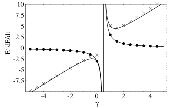
Figure 1: The two solid curves show the theoretically-predicted growth rates for the “vector” [$v$, Eq. (30b)] and one of the scalar [$s2$, Eq. (30c)] polarizations, when those polarizations propagate to the left ($s=-1$). The circles show the results for numerical simulations of the vector wave packet; the crosses show the results for wave packets in the $s2$ polarization. Both predictions agree very well with simulations.

VI Geometric optics limit of KST: PG

In this section, we study another example of the geometric optics formalism: the propagation of radially-propagating wave packets evolving according to the KST 2-parameter formulation of evolution equations, linearized about a Painleve-Gullstrand background.

Our analysis follows the same course as the Rindler case addressed in Sec. V. We first review Painleve-Gullstrand coordinates and the effects of using these coordinates as the background in the linearized KST equations. Subsequently, we construct the explicit form of the polarization and energy equations [Eqs. (II.3.2) and (17)] for packets that propagate radially on the light cone. Finally, in a departure from the Rindler pattern, we also add an analysis of the “zero-speed” modes that propagate against the shift vector.

VI.1 Generating the FOSHLS using a background Painleve-Gullstrand space

A Schwarzchild hole in Painleve-Gullstrand coordinates is characterized by the metric

$$ds^{2}=-dt^{2}+\left(dr+\sqrt{\frac{2}{r}}dt\right)^{2}+r^{2}d\Omega^{2}\;.$$ (32)

We shall use this metric in cartesian spatial coordinates [i.e. $z=r\cos\theta$, $x=r\sin\theta\cos\phi$, $y=r\sin\theta\sin\phi$] as the background spacetime in the KST equations. Linearizing about this background, we obtain the explicit FOSHLS we study in the remainder of this section.

As before, we shall not provide the very complicated derivative-free terms (i.e. $F$) explicitly in this paper. The principal part, however, remains simple by design; in this case, we have [KST Eq. (2.59), along with the definition of $\hat{\partial}_{o}$ in KST Eq. (2.10)]:

$$(\partial_{t}-\beta^{a}\partial_{a})g_{ij} \simeq 0$$ (33a)

$$(\partial_{t}-\beta^{a}\partial_{a})P_{ij}+g^{ab}\partial_{a}M_{bij} \simeq 0$$ (33b)

$$(\partial_{t}-\beta^{a}\partial_{a})M_{kij}+\partial_{k}P_{ij} \simeq 0$$ (33c)

with $\beta^{a}=\sqrt{2/r}\hat{r}^{a}$.

VI.2 Local plane waves and diagonalizing $A^{a}\hat{r}_{a}$

As discussed generally in Sec. II and by way of a Rindler example in Sec. V.2, to understand how wave packets propagate radially we must first understand how local plane waves propagate radially, which in turn requires we diagonalize $A^{a}\hat{r}_{a}$. The basis vectors and eigenvalues are addressed in detail and in a more general setting in Appendix E.1.3. In brief, the eigenvalues are $\omega_{s}(x,k)=s|k|-\beta^{a}k_{a}$ with $s=\pm 1,0$ and the eigenvectors correspond directly to the Rindler results [i.e. Eq. (23), with $x\rightarrow r$; the similarity exists because we can use symmetry without loss of generality to demand the ray propagate radially in the $x$ direction, along $\hat{r}=\hat{x}$].

VI.3 Deriving the polarization and energy equations, for radial propagation on the light cone

Almost half ($12$ of the $30$ characteristic fields) naturally are associated with wave packets that propagate at the speed of light of the background spacetime (i.e. $s=\pm 1$). In other words, they propagate on characteristics that correspond to null curves of the Painleve-Gullstrand metric [Eq. (32)]. For radially propagating characteristics, that means

$$dr/dt=V^{r}_{s}$$ (34)

$$V^{r}_{s}\equiv s-\sqrt{2/r}$$ (35)

with $s=\pm 1$. The resulting null curve structure is shown in Fig. 2.

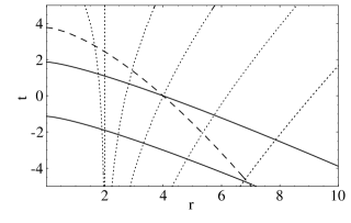
Figure 2: Examples of the three types of radially propagating rays of the KST 2-parameter system linearized about a Painleve-Gullstrand background. The solid lines show rays propagating inward at the speed of light ($V_{r}^{-}$). The dotted lines show rays propagating “outward” at the speed of light ($V_{r}^{+}$). Finally, the dashed curve shows the rays that propagate inside the light cone (at speed $V_{r}^{0}$). The quantities $V_{r}^{s}$ are defined in Eq. (35).

Because both this case and the Rindler case discussed in Sec. V.3 possess rotational symmetry about the propagation axis, the equations governing these two cases prove exceedingly similar. The analysis follows the same course.

VI.3.1 Essential tool: Diagonalizing $P_{s}FP_{s}$ with $s=\pm 1$

As in the Rindler case, we will rewrite the polarization and energy equations by using eigenvectors $f_{s}^{(\mu)}$ of $P_{s}FP_{s}$. Because we again have rotational symmetry about the propagation direction, we can again decompose the eigenvectors into a set of two scalars ($s1$ and $s2$), a 2-vector $v$, and a symmetric-traceless-2-tensor $t$. The eigenvalues may be expressed using

$$\zeta_{s,\mu}\equiv\bar{\zeta}_{s,\mu}/\sqrt{2}r^{3/2}$$ (36)

where the $\bar{\zeta}_{s\mu}$ are defined by

$$\bar{\zeta}_{s,s1} = -3$$ (37a)

$$\bar{\zeta}_{s,s2} = \left[\frac{7}{2}+3\gamma-\frac{(33+91\hat{z}+24\hat{z}^{2})}{4(1+3\hat{z})(1-2\gamma)}\right]$$ (37b)

$$\bar{\zeta}_{s,v} = \frac{3-3\hat{z}-5\gamma}{1-2\gamma}$$ (37c)

$$\bar{\zeta}_{s,t} = 1$$ (37d)

The eigenspaces are, by symmetry, spanned by precisely the same fields as in the Rindler case. In particular, as in the Rindler case the eigenvectors do not change as we move along a ray.

VI.3.2 Polarization equation for $s=\pm 1$

For polarizations which propagate radially on the light cone (i.e. $s=\pm 1$), the polarization equation [Eq. (7)] can be written as

$$0 = \left[\partial_{t}+V_{s}^{r}\partial_{r}\right]d_{s,\alpha}+s\frac{d_{s,\alpha}}{r}$$

$$-\sum_{\beta}d_{s,\beta}\bigg{(}v_{s,\alpha},\;SFv_{s,\beta}\bigg{)}\;.$$

where we make use of Eqs. (84) and (85) to simplify the right side, and where we observe $\partial_{a}\hat{r}^{a}=2/r$.

As in the Rindler case, we may expand the amplitude $\bar{u}=\sum_{\mu}D_{s\mu}f_{s}^{(\mu)}$ in terms of the basis $f_{s}^{(\mu)}$, and thereby arrive at polarization propagation equation precisely analogous to the Rindler result [compare with Eq. (25)]:

$$\left[\partial_{t}+\left(s-\sqrt{\frac{2}{r}}\right)\partial_{r}\right]D_{s\mu}=\left(\zeta_{s\mu}-\frac{s}{r}\right)D_{s\mu}\;.$$ (39)

These equations may be integrated to describe the evolution of polarization along any individual radial ray.

VI.3.3 Energy equation for $s=\pm 1$

Because symmetry guarantees a close similarity between this Painleve-Gullstrand case and the Rindler case, we find the energy $E$ of a geometric-optics-limit solution propagating on the light cone radially inward ($s=-1$) or outward ($s=+1$) can be expressed with precisely the same expression we used in the Rindler case: Eq. (V.3.3). [In this case, we again use a measure $\mu=1$ compatible with the background flat spatial cartesian-coordinate metric.]

The rate of change of this energy, $dE/dt$, can be obtained in two ways. On the one hand, we can directly form $E$, convert to spherical coordinates, differentiate the resulting expression for $dE/dt$, and use Eq. (39). On the other hand, we can find $dE/dt$ using the general expression of Eq. (17), an expression we simplify by using i) the relation between $Q$ and $O_{j}$ given in Eq. (18), ii) the basis $f_{s}^{(\mu)}$ of eigenvectors of $P_{s}FP_{s}$, and iii) the expression [obtained from Eq. (86) and converted from a component to an operator expression]

$$P_{s}\left[\partial_{t}S+\partial_{a}(SA^{a})\right]P_{s}=-\frac{3}{\sqrt{2}r^{3/2}}P_{s}\;.$$ (40)

In either case, we conclude

$$\frac{dE}{dt} = \int d^{3}x\sum_{\mu}|D_{s\mu}|^{2}\frac{2\text{Re}(\bar{\zeta}_{s\mu})-3}{\sqrt{2}r^{3/2}}$$

$$+ \int d^{3}x\;2\text{Re}\left[D_{s,s1}^{*}D_{s,s2}\left(f_{s}^{(s1)}{}^{*},Sf_{s}^{(s2)}\right)\right.$$

$$\quad\times\left.\frac{\bar{\zeta}_{s,s1}^{*}+\bar{\zeta}_{s,s2}-3}{\sqrt{2}r^{3/2}}\right]\;.$$

In particular, for prototypical coherent wave packets – that is, wave packets where $s$ and $\mu$ are the same everywhere in the packet – we can express the growth rate of the energy $E_{s\mu}$ of the wave packet as

$$\frac{1}{E_{s\mu}}\frac{dE_{s\mu}}{dt}=\frac{2\text{Re}(\bar{\zeta}_{s\mu})-3}{\sqrt{2}r^{3/2}}\\$$ (42)

where $r$ is the current location of the packet.

VI.4 Deriving the polarization and energy equations, for radial propagation against the shift vector

The remaining $18$ fields propagate inward against the shift vector, at speed $V_{o}=-\sqrt{2/r}$.

We shall not follow the same pattern we used to address propagation on the light cone [on a Rindler background in Sec. V.3 and on a Painleve-Gullstrand background in Sec. VI.3]. In those sections, we provided extensive discussion and background – the explicit form of the polarization equation; a modified form of the polarization equation in an alternative basis; explicit expressions for the growth rate of energy general geometric-optics solutions; explicit demonstration that PCWP solutions existed – before finally recovering the growth rate of PCWPs. Instead, for pedagogical and other reasons [see Sec. VI.4.3], we shall take a briefer, more practical approach better suited to extracting precisely the information needed to decide when some coherent wave packet can amplify a significant amount within the future domain of dependence.

Specifically, following the arguments at the end of Sec. III.3, we expect that – whether or not PCWPs exist as exact solutions to the polarization equation – when the largest eigenvalue $o_{o\nu}$ of $O_{o}$ is particularly large, a generic coherent wave packet will rapidly converge to a PCWP with $w=f_{o}^{(\nu)}$. In other words, we expect that when the growth rates are large, the growth rate of generic coherent wave packets can be obtained by finding the largest value of $dE/dt/E$ for PCWPs [i.e. the maximum of Eq. (20) over $\mu$].

In short, we continue to evaluate Eq. (20) to get growth rates, though now we trust the results only when the growth rates are large.

VI.4.1 Growth rate of PCWPs

To evaluate the growth rate of PCWPs, we must diagonalize $O_{o}$:

$$O_{o}=P_{o}\left\{F+\frac{1}{2}S^{-1}\left[\partial_{t}S+\partial_{a}(SA^{a})\right]\right\}P_{o}$$

However, from Eq. (40) we know the term in square brackets is diagonal. Therefore, diagonalizing $O_{o}$ to obtain eigenvalues $o_{o\mu}$ and eigenvectors $f_{j}^{(\mu)}$ is equivalent to diagonalizing $P_{o}FP_{o}$ for eigenvalues $\zeta_{o\mu}$ and eigenvectors $f_{o}^{(\mu)}$ . The eigenvalues of the two operators are related by

$$o_{o\mu}=\zeta_{o\mu}-\frac{3}{2\sqrt{2}r^{3/2}}\;$$ (43)

We shall express the eigenvalues $\zeta_{o\mu}$ of $P_{o}FP_{o}$ in terms of the dimensionless rescaled quantities $L_{\mu}$, defined implicitly by

$$\zeta_{0\mu}=L_{\mu}\times\sqrt{2}/r^{3/2}$$ (44)

Substituting Eq. (43) into the general expression for the growth rate of PCWPs [Eq. (20)], we find that a PCWP in the polarization $\mu$ will have energy grow at rate

$$\frac{1}{E_{o\mu}}\frac{dE_{o\mu}}{dt}=\left[2\text{Re}(L_{\mu})-\frac{3}{2}\right]\frac{\sqrt{2}}{r^{3/2}}$$ (45)

where $r$ is the instantaneous location of the packet.

VI.4.2 Essential tool: Diagonalizing $P_{o}FP_{o}$

To obtain explicit growth rate expressions using Eq. (45), we need the eigenvalues of $P_{o}FPo$, expressed according to Eq. (44).

As in the previous two cases, the eigenspaces of $P_{o}FP_{o}$ may be decomposed into distinct classes, depending on their symmetry properties of rotation about the propagation axis. These spaces are as follows:

• Helicity-0 a 4-dimensional space of rotational scalars (“helicity-0” states), with eigenvalues given by Eq. (44) with

  $$L_{s1,s2} = \frac{-1+3\hat{z}+18\hat{z}^{2}\pm\sqrt{3}\sqrt{Y_{1}}}{4(1+3\hat{z})}$$ (46a)

  $$L_{s3} = \frac{1}{4}(-30+19\eta+12\hat{z}-6\eta\hat{z})$$ (46b)

  $$L_{s4} = \frac{3}{2}(1+2\hat{z})$$ (46c)

  Here, we use $\eta\equiv-2/(\gamma-1/2)$ and $Y_{1}$ given according to an expression listed below [Eq. (47)].

• Helicity-1 an 8-dimensional space of rotational 2-vectors (“helicity-1” states), with doubly-degenerate eigenvalues given by

  $$L_{v1} = -2$$ (46d)

  $$L_{v2} = \frac{1}{2}(1+6\hat{z})$$ (46e)

  $$L_{v3,v4} = \frac{3}{8}(5+8\hat{z})+\frac{\eta(13+83\hat{z}+84\hat{z}^{2})}{32(1+3\hat{z})}$$ (46f)

  $$\pm\frac{\sqrt{Y_{2}}}{32(1+3\hat{z})}$$

  Again, we use $\eta\equiv-2/(\gamma-1/2)$. The expression for $Y_{2}$ is given below [Eq. (48)].

• Helicity-2 a 4-dimensional space of symmetric-traceless-2-tensors (“helicity-2” states), with doubly-degenerate eigenvalues given by

  $$L_{t1} = \frac{3}{2}(1+2\hat{z})$$ (46g)

  $$L_{t2} = 2+3\hat{z}$$ (46h)

• Helicity-3 and finally a 2-dimensional space of helicity-3 states, with eigenvalue

  $$L_{3}=3(1+\hat{z})$$ (46i)

In the above discussion, $Y_{1,2}$ are defined by

$$Y_{1} = (1+3\hat{z})(-5+5\hat{z}+24\hat{z}^{2}+36\hat{z}^{3})$$ (47)

$$Y_{2} = 1296(1+3\hat{z})^{2}+\eta^{2}(13+83\hat{z}+84\hat{z}^{2})^{2}$$ (48)

$$-24\eta(1+3\hat{z})(89+199\hat{z}+132\hat{z}^{2})$$

and we use the shorthand $\eta\equiv-2/(\gamma-1/2)$.

VI.4.3 Aside: Why can’t we follow the previous pattern?

Unlike all cases previously discussed, a handful of the eigenvectors depend weakly on position. As a result, the use of a basis which diagonalizes $O_{o}$ does not offer as dramatic a simplification as it did in our earlier analyzes of the polarization equation [Sections V.3 and VI.3]. To be explicit, if we rewrite the polarization equation in the basis $f_{o}^{(\mu)}$ in the fashion of those earlier analyzes, we obtain [see Eq. (C.1)]

$$\sum_{\nu}D_{o\nu}M_{\mu\nu}=\left(\partial_{t}+V_{o}^{a}\partial_{a}+\frac{1}{2}\partial_{a}V_{o}^{a}-o_{o\mu}\right)D_{o\mu}$$ (49)

for $M_{\mu\nu}$ some nonzero, position-dependent matrix coupling the various $D_{o\mu}$.

VII Transients and limitations on numerical simulations: Rindler

In earlier sections, we developed – in general [Sections II, III, and IV] and for specific examples [e.g., Sec. V analyzes propagation of transients according to the KST 2-parameter formulation of Einstein’s equations, linearized about a Rindler background] – tools to analyze the growth of special (i.e. prototypical coherent wave packet) geometric-optics-limit transient solutions. In this section, we demonstrate how these tools can be used to discover when a particular formulation of Einstein’s equations [here, some specific member of the KST 2-parameter system] which is linearized about a specific background [here, flat space in Rindler coordinates] admits some massively-amplified transient solution.

Specifically, in this section we apply the general tools developed in an earlier section [Sec. V] to determine the largest possible amplification of a prototypical coherent wave packet while it remains within the future domain of dependence of some initial data slice. In Sec. VII.1 we describe the initial data slice we chose and the subset of transient solutions we studied. In Sec. VII.2, we apply the tools developed in an earlier section [Sec. V] to determine the amplification of each transient. We also find an expression for the largest possible amount a transient can amplify. Finally, in Sec. VII.2, we invert our expression to determine which pairs of KST parameters ($\hat{z}$, $\gamma$) admit transients that amplify in energy by more than $10^{32}$ (i.e. in amplitude by more than $10^{16}$).

VII.1 Transients studied

We limit attention to the future domain of dependence of the initial-data slice $x\in[0.01,1]$ at $t=0$. Since the KST 2-parameter formulation has fields which propagate at (but no faster than) the speed of light, the future domain of dependence of this slice is precisely what we would obtain using Einstein’s equations: a region bounded by the two curves $x_{-}\equiv 0.01\exp t$ and $x_{+}\equiv\exp(-t)$. This region is shown in Fig. 3. The future domain of dependence extends to time

$$T_{\text{max}}\equiv\ln 10\;,$$ (50)

at which point the two bounding curves curves intersect.

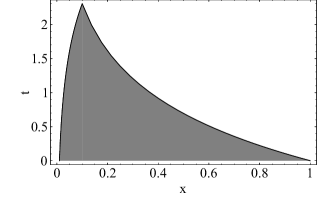
Figure 3: The shaded region is the future domain of dependence of the region $x\in[0.01,1]$ for the KST 2-parameter formulation of evolution equations linearized about a Rindler background. Transients are any solutions which are defined in this region. We study all the prototypical coherent wave packets which propagate on the light cone (i.e. according to $dx/dt=\pm x$).

.

Geometric-optics solutions are defined on rays [i.e. solutions to Eq. (8)]. While three classes of rays exist in this region – those ingoing at the speed of light ($dx/dt=-x$); those outgoing at the speed of light ($dx/dt=+x$); and those which have fixed coordinate position – we for simplicity chose to study only the amplification of transients that propagate on the light cone.

VII.2 Amplification expected

For each ray that propagates on the light cone ($dx/dt=\pm x$) within the future domain of dependence, and for each polarization on that ray, we can compute the amplification in energy. If $R_{s,\mu}\equiv E_{s\mu}^{-1}dE_{s\mu}/dt$ [see Eq. (30)], we can express the ratio of energy of the wave packet when it exits the future domain of dependence at time $t_{\text{out}}$ to the initial energy at time $t=0$ as

$${\cal A}_{s\mu}(x_{o})=E_{s\mu}(t_{\text{out}})/E_{s\mu}(0)=\exp\left(t_{\text{out}}R_{s\mu}\right)\;.$$

We have explicit expressions for $R_{s\mu}$; we can compute $t_{\text{out}}(x_{o},s)$ for each initial point $x_{o}$ and for each propagation orientation (i.e. for each $s$); and we therefore can maximize $A_{s\mu}(x_{o})$ over all possible choices of initial location ($x_{o}$), propagation direction ($s$), and polarization ($\mu$) to find the largest possible ratio ${\cal A}$ of initial to final prototypical coherent wave packet energy.

In fact, because for each polarization of prototypical coherent wave packet, the growth rates of energy is independent of time and space, the largest amplifications possible always occur along the longest-lived rays – in other words, along the two bounding rays $x_{+}$ and $x_{-}$, which both extend to $t_{\text{out}}=T_{\text{max}}$. Therefore, we conclude that, while within the future domain of dependence of the slice $x\in[0.01,1]$, the largest amount the energy of any prototypical coherent wave packet can amplify is given by the factor

$${\cal A}=\exp(T_{\text{max}}R_{\text{Rind}})$$ (51)

where $R_{\text{Rind}}$ is given by

$$R_{\text{Rind}} \equiv \max_{\mu,s}R_{s\mu}=\max_{\mu,s}\left[2\text{Re}(\zeta_{s\mu})+s\right]$$

$$= {\max}\left(1,\left|2\frac{1+\gamma}{-1+2\gamma}-1\right|,\left|2\frac{1+2\gamma^{2}}{-1+2\gamma}-1\right|\right)$$

KST formulations which definitely possess some ill-behaved transient solution when linearized about Rindler

Finally, we can invert Eq. (51) to find those combinations of KST parameters ($\hat{z}$, $\gamma$) which permit some transient (in particular, some prototypical coherent wave packet) to increase in energy by more than a factor $10^{32}$ (i.e. $10^{16}$ in amplitude). The condition may be expressed as either ${\cal A}>10^{32}$ or, equivalently, as $R_{\text{Rind}}>32$. The function $R_{\text{Rind}}$ is shown in Fig. 4, along with the line $R_{\text{Rind}}=32$.

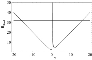
Figure 4: The solid curve is the theoretical prediction for the largest growth rate of wave packets that propagate on the light cone [Eq. (VII.2)]. The horizontal line is the value $32$. According to arguments made in Sec. VII.2, those $\gamma$ which have $R_{\text{Rind}}>32$ have some prototypical coherent wave packet which, in the future domain of dependence, amplifies in energy by more than $10^{32}$.

Therefore, we know that some transient can amplify in energy by more than $10^{32}$ if i) $\gamma>(33+\sqrt{949})/4$, ii) $\gamma<-(31+\sqrt{1077})/4$, or iii) $\gamma>29/64$ and $\gamma<(33-\sqrt{949})/4$.

VII.3 Relevance of our computation to numerical simulations

We have demonstrated that the KST 2-parameter formulation of Einstein’s equations always admits, at any instant, prototypical coherent wave packet solutions which grow exponentially in time. Generically, we expect that at each instant (including in the initial data) these solutions are excited by errors in the numerical simulation (e.g. truncation and roundoff). They then propagate and grow; eventually, they reach the computational boundary.

Our calculations above describes the largest amount any such wave packet solution could possibly grow by the time it reaches the computational boundary. If that amplification factor is sufficiently large that the wave packets reach “unit” amplitude (i.e. whatever magnitude is needed to couple to nonlinear terms strongly), here conservatively assumed to be $10^{16}$, then we expect any simulation using that particular combination of KST parameters will quickly crash.

Aside: What happens to PCWPs at late times?

Eventually, the wave packets excited by numerical errors will reach the computational boundary. What happens afterward depends strongly on the precise details of the boundary conditions.

For example, maximally-dissipative boundary conditions (i.e. the time derivatives of all outgoing characteristic fields are set to zero) will allow the wave packet to leave the computational domain entirely (with some small amount of reflection that goes to zero in the geometric-optics limit). In this case, at late times no transient will ever amplify by more than the amount described above (in Sec. VII.2).

On the other hand, other choices for boundary conditions could cause wave packets to reflect back in to the computational domain. In these circumstances, the outcomes are far more varied – at late times, the wave packet could potentially grow, could decay to zero, or could enter a repetitive cycle where on average its amplitude is constant.

Therefore, without some more specific proposal for boundary conditions, we cannot make useful statements regarding the late-time development of this instability process – or, in other words, we cannot study the growth of coherent wave packets for more than a light crossing time.

VIII Transients and limitations on numerical simulations: PG

In this section, we provide another example of how tools developed earlier for the analysis of prototypical coherent wave packets – in general [Sections II, III, and IV] and for specific examples [e.g., Sec. VI analyzes propagation of transients according to the the KST 2-parameter formulation of Einstein’s equations, linearized about a Painleve-Gullstrand background] – can be applied to discover which formulations of Einstein’s equations permit ill-behaved transients.

Specifically, in this section we study the propagation coherent wave packets in the 2-parameter KST form of Einstein’s evolution equations, linearized about Schwarzchild written in Painleve-Gullstrand (PG) coordinates. The theory needed to understand the propagation and growth of radially-propagating coherent wave packets has been developed in an earlier section [Sec. VI]. We apply our techniques to a handful of coherent wave packet transient solutions, to discover conditions on the two KST parameters ($\hat{z}$, $\gamma$) which permit amplification of those transients’ energy by a factor $1/\epsilon_{e}^{2}$ for $\epsilon_{e}=10^{-16}$.

To provide concrete examples of estimates, we assume the initial data slice contains the region $r\in[2,10]$. So any influence from boundary conditions cannot muddle our computations, we limit attention to coherent which are defined in the future domain of dependence of that slice.

VIII.1 Transients studied

We limit attention to the future domain of dependence of the region $r\in[2,10]$ at $t=0$. Since the KST 2-parameter formulation has fields which propagate at (but no faster than) the speed of light, the future domain of dependence of this slice is precisely what we would obtain using Einstein’s equations: the region shown in Fig. 5.

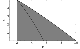
Figure 5: The shaded region is the future domain of dependence of the region $r\in[2,10]$ for the KST 2-parameter formulation of evolution equations. Transients are any solutions which are defined in this region. For reasons emphasized in the text, the rays that last for the longest coordinate time prove particularly helpful. These rays are the left and right boundaries (i.e. the horizon and a ray that propagates inward at the speed of light from $r=10$) and one ray propagating against the shift vector which emanates from their intersection.

In particular, the future domain of dependence is bounded on the left by the generators of the horizon (trapped at $r=2$) and on the right by rays travelling inward at the speed of light. This ingoing ray reaches $r=2$ at the endpoint of the future domain of dependence, at time $t=t_{\text{max}}$ defined by

$$t_{\text{max}} \equiv \int_{2}^{10}\frac{dr}{1+\sqrt{2/r}}$$

$$= 4[3-\sqrt{5}+\text{csch}^{-1}(2)]\approx 4.98$$

In our future domain of dependence, we have three classes of solutions to the ray-propagation equation [Eq. (8)]: those ingoing at the speed of light ($V_{-}=-1-\sqrt{2/r}$); those ingoing with the shift ($V_{o}=-\sqrt{2/r}$); and those outgoing ($V_{+}=1-\sqrt{2/r}$) [Eq. (35)].

VIII.2 Amplification conditions

For each of the three classes of rays ($s=\pm 1,0$) propagating radially in the future domain of dependence [Fig. 5] and for each polarization on that ray, we can compute the amplification in energy using $R_{s\mu}\equiv E_{s\mu}^{-1}dE_{s\mu}/dt$ [see Eqs. (42) and (45)]. Specifically, for a wave packet starting at $r=r_{o}$ at time $t=0$, propagating in the $s$-type congruence and in the polarization $\mu$, the energy at the time $t_{\text{out}}(r_{o},s)$ the ray exits the future domain of dependence is larger than the initial energy by a factor

$${\cal A}_{s\mu}(r_{o}) \equiv E_{s\mu}(t_{\text{out}})/E_{s\mu}(0)$$ (54a)

$$\ln{\cal A}_{s\mu}(r_{o}) = \int_{0}^{t_{\text{out}}}dt\;R_{s\mu}=\int_{r_{o}}^{r_{\text{out}}}\frac{dr}{V_{r}^{s}}R_{s\mu}$$ (54b)

We then search over all $r_{o}$, over all propagation directions $s$, and over all polarizations $\mu$ to find the largest amplification factor ${\cal A}$.

In fact, as in the Rindler case, we immediately know which rays produce the largest possible amplification, so we can perform the maximization by inspection.

• Outgoing at light speed: Since the amplification of energy increases as $r$ gets smaller ($dE/dt/E\propto 1/r^{3/2}$) and with the duration of the ray in time, manifestly the generator of the horizon – with both the longest duration and the smallest $r$ of all outgoing rays –will provide the largest possible amplification.

  Since the ray of interest has fixed radial location $r=2$, we find $\zeta_{+,\mu}$ is constant for all polarizations. Thus, the energy of a prototypical coherent wave packet in polarization $\mu$ increases by a factor $A_{+\mu}$, for $A_{+\mu}=\exp(t_{\text{max}}\zeta_{+\mu})$. In other words,

  $$\ln{\cal A}_{\mu} = \left[2\text{Re}(\bar{\zeta}_{+,\mu})-3\right][3-\sqrt{5}+\text{csch}^{-1}(2)]$$

  $$\approx 1.245\left[2\text{Re}(\bar{\zeta}_{+,\mu})-3\right]$$

  [The values for each $\bar{\zeta}_{+\mu}$ are given in Eq. (37).]

• Ingoing at light speed: The longest ray – namely, the right boundary of the future domain of dependence – permits the greatest possible amplifications. Thus, among all possible ingoing rays, the largest amplification factor for the polarization $\mu$ is given by ${\cal A}_{-\mu}$:

  $$\ln{\cal A}_{-\mu} = \left[2\text{Re}(\bar{\zeta}_{-,\mu})-3\right]\cdot\frac{\ln 5-2\text{csch}^{-1}(2)}{2}$$

  $$\approx 0.323\left[2\text{Re}(\bar{\zeta}_{-,\mu})-3\right]$$

  [The values for each $\bar{\zeta}_{-\mu}$ are given in Eq. (37).]

  Note that since $\zeta_{-\mu}=\zeta_{+\mu}$, the outgoing transients trapped on the horizon grow more than the ingoing ones over the same time interval.

• Ingoing with lapse: The amplification of energy increases both with ray length and with proximity to $r=0$ (since growth rates go as $1/r^{3/2}$). Thus, the longest ray propagating at this speed contained in the future domain of dependence gives the best chances. That ray starts with $r=r_{L}$, with $r_{L}$ defined so the ray terminates at the horizon at $t=t_{\text{max}}$:

  $$r_{L}\equiv\left[\frac{\left(4+3t_{\text{max}}\right)^{2}}{2}\right]^{1/3}$$ (57)

  Thus, we find the largest possible amplification among those polarizations that have $s=0$ to be given by ${\cal A}_{0\mu}$:

  $$\ln{\cal A}_{o\mu} = \left[2\text{Re}(L_{\mu})-\frac{3}{2}\right]\times\int_{2}^{r_{L}}\frac{dr}{\sqrt{2/r}}\frac{\sqrt{2}}{r^{3/2}}$$ (58)

  $$= \left[2\text{Re}(L_{\mu})-\frac{3}{2}\right]\ln\left(r_{L}/2\right)$$

  [The values for each $L_{\mu}$ are given in Eq. (46).]

VIII.3 Results: Some KST parameters which have transients which amplify by $10^{32}$

Under the proper choice of KST parameters, shown shaded in Fig. 6, one of the three types of ray ($s=\pm 1,0$) may admit some prototypical coherent wave packet of polarization $\mu$ whose energy amplifies by $10^{32}$ [i.e. ${\cal A}_{s\mu}\geq 10^{32}$]. The clear region in Fig. 6 indicates KST parameters for which we have not yet found a transient which amplifies by $10^{32}$.

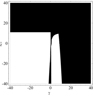
Figure 6: The shaded region indicates those KST parameters which produce some radially-propagating prototypical coherent wave packets which amplify their energy by greater than $10^{32}$ within the future domain of dependence of the slice $r\in[2,10]$. Note a large proportion of parameter space has been excluded.

VIII.4 Generalizations of our method which could generate stronger constraints on KST parameters

With our extremely conservative approach – eliminating those formulations with wave-packet solutions which amplify by $10^{32}$ in the future domain of dependence – we have already eliminated a broad region of parameter space. By relaxing some of our very restrictive assumptions, we expect we could discard still more KST parameters:

1. Lower amplification cutoff: Currently, we require an enormous amplification before we eliminate a formulation; relaxing the requirement on amplification excludes more systems.

2. Consider more transients Currently, we compute the amplification of only a handful of transients; a consideration of other transients (for example, in the neighborhood of circular photon orbits in PG) may allow us to exclude additional parameters.

3. Consider a larger region Currently, we limit attention only to the future domain of dependence of the initial data slice. Certain rays, however, remain within the computational domain for far longer. For example, in the PG case, rays near the horizon remain in the domain for arbitrarily long; even the slowly-infalling rays last substantially longer than the domain of dependence. Therefore, by considering the amplification of transients over a longer interval, we will discover significantly greater amplification and thus exclude a significantly broader class of formulations of Einstein’s equations.

4. Combine with boundary conditions Finally, if we determine how geometric-optics solutions interact with boundary conditions, we can generalize our approach and address the late-time stability properties of the evolution equations – or, in other words, address the stability properties of the full initial-plus-boundary value problem.

IX Conclusions

In this paper, we have demonstrated that certain transients (prototypical coherent wave packets) can be used to veto a significant range of proposed formulations of Einstein’s equations. We have described in considerable pedagogical detail precisely how to construct expressions for (or estimates of) the growth rate of prototypical coherent wave packets [i.e. Eq. (20)], verify those estimates, and employ them to veto proposed formulations of Einstein’s equations. These expressions employ no free parameters or knowledge of the solution, aside from a choice of plausible rays to examine. Moreover, despite the sometimes exhaustive details provided in Sections V and VI, the key tool – the growth rate of prototypical coherent wave packets [Eq. (20)] – is easy to apply, with little conceptual, notational, or computational overhead (see, for example, the brief Sec. VI.4.1 and its application in Sec. VIII). Whether they are used conservatively, as in this paper, or generalized along the lines suggested in Sec. VIII.4 (i.e. using more rays and larger fragments of spacetime), we believe these techniques will provide a useful way to bound the number of proposed formulations before further tests are conducted (for example by the more ambitious Lindblom-Scheel energy-norm method) to decide whether a given formulation can produce effective simulations.

While our the specific examples of analyses in this paper have employed linearizations of the field equations themselves, we could just as well linearize a FOSH system representing evolution equations for the constraint fields [see, for example, KST Eqs. (2.40-2.43)]. The evolution equations for the constraints have been emphasized by many other authors as an probe of unphysical behavior. Since the general arguments of Sections II, III, and IV do not depend on the precise FOSHLS used, we can perform a calculation following the same patterns as (for example) Sec. VIII to discover ill-behaved formulations.

In this paper, we have also discovered curious properties of modes trapped on the horizon of a Schwarzchild hole in PG coordinates (Sec. VIII). Analytically, we would expect that, if any growth rate for modes trapped on the horizon were positive, then these modes should grow without bound and be present in the evolution at late times. Numerically, however, we know that no resolved wave packets can appear at late times: such solutions would have to initiate arbitrarily close to the horizon, inconsistent with resolved, finite-resolution initial data. Still, marginally-resolved solutions of similar character could potentially behave in an implementation-dependent fashion, seeding outgoing modes which then propagate and amplify into the domain for all time. We shall explore this possibility in a future paper.

Appendix A Useful identities used in the text

A.1 An alternative approach to the group velocity

The eigenequation which defines the natural polarization spaces $B_{j}$ and their associated eigenvalues $\omega_{j}$,

$$A^{a}p_{a}v_{j,\alpha}=\omega_{j}v_{j,\alpha}$$

for each $v_{j,\alpha}\in B_{j}$ (cf. Sec. II.1), may be alternatively expressed as

$$A^{a}(x)p_{a}P_{j}(x,p)=\omega_{j}(x,p)P_{j}(x,p)\;.$$ (59)

for $P_{j}$ the projection operator to the $j$th eigenspace of $A^{a}p_{a}$. Differentiate this expression relative to $p_{b}$, then apply $P_{j}$ from the left, to find

$$P_{j}A^{a}P_{j}=\frac{\partial\omega_{j}}{\partial p^{a}}P_{j}=V_{j}^{a}P_{j}\;.$$ (60)

Equivalently, if $v_{j,\alpha}$ are a collection of basis vectors for the $j$th eigenspace which are orthonormal relative to the inner product generated by $S$,

$$(v_{j,\beta},SA^{a}v_{j,\alpha})=\delta_{\alpha\beta}V_{j}^{a}\;.$$ (61)

A.2 The no-rotation condition

In Section II.3.2, we claim we can always find a basis for $B_{j}$ at each point in the neighborhood of a given ray which satisfies the no-rotation condition [Eq. (10)]:

$$\left(v_{j,[\alpha},S(\partial_{t}+A^{a}\partial_{a})v_{j,\beta]}\right)=0$$ (62)

for all $\alpha$, $\beta$. In this section, we demonstrate explicitly how to construct a basis which satisfies both the no-rotation condition and which remains orthonormal.

If the right-hand side term in Eq. (62) is not zero in the basis $v_{j,\alpha}$, we attempt to choose a new basis

$$v_{j,\bar{\alpha}}\equiv R_{\bar{\alpha}\alpha}v_{j,\alpha}$$

such that Eq. (10) is satisfied by the new basis and moreover such that the new basis is orthonormal. In particular, if the no-rotation condition is satisfied in the new basis, then (because $P_{j}A^{a}P_{j}=V_{j}^{a}$) we know

$$0 = \sum_{\alpha\beta}R_{\bar{\alpha}\alpha}R_{\bar{\beta}\beta}\left(v_{j,[\alpha},S(\partial_{t}+A^{a}\partial_{a})v_{j,\beta]}\right)$$

$$+ R_{[\bar{\alpha}\alpha}\sum_{\alpha}(\partial_{t}+V_{j}^{a}\partial_{a})R_{\bar{\beta}]\alpha}\;.$$

[In the second term above, the antisymmetrization is over only the barred indicies $\bar{\alpha}$ and $\bar{\beta}$.] On the other hand, if the basis is orthonormal, then $\sum_{\alpha}R_{\bar{\alpha}\alpha}R_{\bar{\beta}\alpha}=\delta_{\bar{\alpha}\bar{\beta}}$, implying

$$\sum_{\alpha}R_{(\bar{\alpha}\alpha}(\partial_{t}+V_{j}^{a}\partial_{a})R_{\bar{\beta})\alpha}=0\;.$$

[In the above, the operator is symmetrized over the indicies $\bar{\alpha}$ and $\bar{\beta}$.] Therefore, combining the two, we conclude that if the new basis is both orthonormal and satisfies the no-rotation, the matrix $R$ must satisfy the ordinary differential equation

$$(\partial_{t}+V_{j}^{a}\partial_{a})R_{\bar{\alpha}\alpha}=-\left(v_{j,[\alpha},S(\partial_{t}+A^{a}\partial_{a})v_{j,\beta]}\right)R_{\bar{\alpha}\beta}$$

subject to initial data $R_{\bar{\alpha}\alpha}=\delta_{\bar{\alpha}\alpha}$. Solutions for $R$ and thus $v_{j,\bar{\alpha}}$ exist in the neighborhood of a ray.

A.3 Reorganizing inner products for the polarization equation

In this section, we describe how to rearrange matters so the last term in Eq. (7) – namely,

$$\bigg{(}v_{j,\alpha},\;S(\partial_{t}+A^{a}\partial_{a})v_{j,\beta}\bigg{)}\;$$ (64)

– has a simpler form. If we choose a basis that satisfies the no-rotation condition [Eq. (10)], the antisymmetric part of this matrix is zero. Further, we may express the symmetric part of this expression by using the relations

$$\partial_{t}(v_{j,\alpha},Sv_{j,\beta}) = (v_{j,\alpha},S{\partial}_{t}v_{j,\beta})$$

$$+(v_{j,\beta},S{\partial}_{t}v_{j,\alpha})$$

$$+\left(v_{j,\alpha},(\partial_{t}S)v_{j,\beta}\right)$$

$$\partial_{a}(v_{j,\alpha},SA^{a}v_{j,\beta}) = (v_{j,\alpha},SA^{a}{\partial}_{a}v_{j,\beta})$$

$$+(v_{j,\beta},SA^{a}{\partial}_{t}v_{j,\alpha})$$

$$+\left(v_{j,\alpha},\left(\partial_{a}SA^{a}\right)v_{j,\beta}\right)$$

[where we have observed that $SA^{a}$ and $A^{a}$ are symmetric relative to the canonical inner product] and the expressions

$$(v_{j,\alpha},Sv_{j,\beta}) = \delta_{\alpha\beta}$$ (67)

$$(v_{j,\alpha},SA^{a}v_{j,\beta}) = \delta_{\alpha\beta}V_{j}^{a}$$ (68)

[i.e. orthogonality and Eq. (61)]. These relations tell us that, if the no-rotation condition is satisfied,

$$\left(v_{j,\alpha}\right., \left.S(\partial_{t}+A^{a}\partial_{a})v_{j,\beta}\right)=$$

$$\frac{1}{2}\delta_{\alpha,\beta}\partial_{a}V^{a}(\vec{x},\vec{k}(x))-\frac{1}{2}\left(v_{j,\alpha},\left(\partial_{t}S+{\partial}_{a}SA^{a}\right)v_{j,\beta}\right)$$

Our notation for the first term on the right side (i.e. the divergence of the group velocity) is chosen to emphasize that the derivative $\partial_{a}$ acts on all the dependence on $\vec{x}$ – in particular, on any variation of $k_{a}=\partial_{a}\phi$ with $\vec{x}$.

Appendix B Demonstrating that the ray-optics approach provides high-quality approximate solutions to the FOSHLS

For any fixed initial data, the ray-optics solution obtained in Sec. II will break down at some point along each ray. In this section, we estimate how long a solution obtained by solving Eq. (7) can be trusted.

Specifically, in Sec. B.1 we express the FOSHLS [Eq. (2)] using alternative variables better-suited to describing the geometric-optics solution. Next, in Sec. B.2 we survey the various orders of magnitude that arise in the problem. Using those orders of magnitude, in Sec. B.3 we estimate the error in Eq. (2) that occurs when a geometric optics solution is substituted for $u$ (e.g. we estimate how close the norm of the left side is to zero). Finally, knowing how much error we make when using a geometric-optics solution, in Sec. B.4 we estimate how errors involved in a geometric-optics approximation grow; we therefore discover how long we can trust a purely geometric-optics-based evolution.

B.1 Review: Writing equations in terms of $\phi$ and $d_{l,\alpha}$

In Equations (5) and (6) we describe how to parameterize the $N$-dimensional state vector $u$ by using $N$ functions $d_{l,\alpha}$ and one additional function $\phi$. If we insert this substitution into the original FOSHLS [Eq. (2)], then dot the results against each of the orthonormal basis vectors $v_{l,\alpha}$, we obtain the equations

$$0 = i(v_{l,\alpha},S\bar{u})\left[\partial_{t}+V_{l}^{a}\partial_{a}\right]\phi$$

$$+\bigg{(}v_{l,\alpha},\;S(\partial_{t}+A^{a}\partial_{a}-F)\bar{u}\bigg{)}$$

$$= id_{l,\alpha}\left[\partial_{t}+V_{l}^{a}\partial_{a}\right]\phi$$

$$+\partial_{t}d_{l,\alpha}+\sum_{m}\sum_{\beta}(v_{l,\alpha},\;SA^{a}v_{m,\beta})\partial_{a}d_{m,\beta}$$

$$+\sum_{m}\sum_{\beta}d_{m,\beta}\bigg{(}v_{l,\alpha},\;S(\partial_{t}+A^{a}\partial_{a}-F)v_{m,\beta}\bigg{)}\;.$$

In the above, we have observed that $A^{a}$ is symmetric relative to the inner product generated by $S$ and that $v_{j,\alpha}$ is an eigenvector of $A^{a}\partial_{a}\phi$ with eigenvalue $\omega_{j}=V^{a}_{j}\partial_{a}\phi$. We can further reorganize this equation by pulling out all terms that involve $d_{l}$ explicitly, and also by using Eq. (60) to simplify $(v_{l,\alpha},SA^{a}v_{l,\beta})=V_{l}^{a}\delta_{\alpha\beta}$:

$$0 = id_{l,\alpha}\left[\partial_{t}+V_{l}^{a}\partial_{a}\right]\phi+\left[\partial_{t}+V_{l}^{a}\partial_{a}\right]d_{l,\alpha}$$

$$+\sum_{\beta}d_{l,\beta}\bigg{(}v_{l,\alpha},\;S(\partial_{t}+A^{a}\partial_{a}-F)v_{l,\beta}\bigg{)}$$

$$+\sum_{m\neq l}\sum_{\beta}(v_{l,\alpha},\;SA^{a}v_{m,\beta})\partial_{a}d_{m,\beta}$$

$$+\sum_{m\neq l}\sum_{\beta}d_{m,\beta}\bigg{(}v_{l,\alpha},\;S(\partial_{t}+A^{a}\partial_{a}-F)v_{m,\beta}\bigg{)}\;.$$

B.2 Natural scales used in order-of-magnitude estimates

To make order-of-magnitude arguments regarding the solution, we need to understand how the natural length scales of the problem enter into it.

Rather than complicate the order-of-magnitude calculation unnecessarily, we shall for simplicity proceed as if there existed only one characteristic speed. In other words, we shall freely convert between space and time units by using the norm of $A^{a}$; for example, we can interpret $\tau_{F,n}|A|$ as a natural length scale. Finally, for brevity, we shall assume space and time units are chosen so $|A|\sim 1$.

Even with the above simplification, many natural scales arise in the problem, including the magnitude of $F$; the natural length and time scales on which $F$ and $A$ vary; and the length scale on which the initial data varies. Again, for simplicity we shall summarize all these scales by only two numbers:

• “Length” scale ($L$) We define the natural “length” scale to be the natural time scale that enters on the right side of Eq. (7). To be explicit, $L$ is the smaller of $|d|/|A||\partial_{a}d|$ and $1/|F|$.

• “Variation” scale ($\tau_{\text{vary}}$) The remaining scales do not arise directly in the equation. They affect the propagation of the wave packet only because they determine the rate at which terms in the equation are modulated as the wave packet propagates in space and time. We therefore call the smallest of the remaining scales the variation scale ($\tau_{\text{vary}}$); its value is the smallest of the length and time scales on which $A$ and $F$ vary.

B.3 Degree to which ray-optics solution satisfies the FOSHLS

Using the above rough estimates ($L$ and $\tau_{\text{vary}}$) to characterize the magnitude of terms both used and neglected, we find that geometric-optics solutions [Eq. (7)] very nearly satisfy the full FOSHLS [Eq. (2), alternatively expressed as Eq. (B.1)]. To be explicit, when we insert a geometric-optics solution which propagates in the $j$th polarization [i.e. a solution to Eq. (7)] into Eq. (B.1), we find the following:

$$0 = id_{l,\alpha}(\omega_{l}-\omega_{j})+\left[\partial_{t}+V_{l}^{a}\partial_{a}\right]d_{l,\alpha}$$

$$+\sum_{\beta}d_{l,\beta}\bigg{(}v_{l,\alpha},\;S(\partial_{t}+A^{a}\partial_{a}-F)v_{l,\beta}\bigg{)}$$

$$+\sum_{m\neq l}\sum_{\beta}(v_{l,\alpha},\;SA^{a}v_{m,\beta})\partial_{a}d_{m,\beta}$$

$$+\sum_{m\neq l}\sum_{\beta}d_{m,\beta}\bigg{(}v_{l,\alpha},\;S(\partial_{t}+A^{a}\partial_{a}-F)v_{m,\beta}\bigg{)}$$

[Here, we have used Eq. (7a) and the definition of $\omega_{j}$ to simplify the first term.]

We have two circumstances:

• When $l=j$, the first three terms precisely cancel [see Eqs. (7a) and (7)]. The only terms remaining are of order $d_{m,\beta}$ $m\neq j$.

• On the other hand, when $l\neq j$, the first term does not cancel. Rather, it is large, because $\partial_{a}\phi$ is large (i.e. we are in the short-wavelength limit), and the $\omega_{l}$ are proportional to $\partial_{a}\phi$.

  For brevity, assume the eigenvalues of $A^{a}$ are of comparable magnitude, so to order of magnitude $\omega_{j}\sim\omega_{l}\sim\omega\sim\omega_{j}-\omega_{l}$. We may then express the equation when $l\neq j$ as

  $$0={\cal O}(\omega d_{l\beta})+{\cal O}(d_{j,\alpha}/L)$$

  The second terms will force the first terms, generally, to be nonzero.

From the second case, we know that when $l\neq j$, $|d_{l}|\sim{\cal O}(|d_{j}|/L\omega)$. Combining this result with the first equation, we conclude that when we use our trial solution, we are ignoring terms of order $|d_{j}|/L^{2}\omega$ when $l=j$ and terms of order and $|d_{j}|/L$ when $l\neq j$.

B.4 Length of time ray-optics solution can be trusted

To estimate the integrated effects the neglected terms have on the diagonal and off-diagonal polarization amplitudes $d_{j,\alpha}$ and $d_{l,\alpha}$, respectively, we integrate the previous equations.

When $l\neq j$, we have a DE of form

$$\frac{d}{ds}d_{l,\beta}+id_{l,\beta}\Delta\omega+{\cal O}(|d_{j}|/L)=0$$

where we neglect smaller terms, where $d/ds=\partial_{t}+V^{a}_{j}\partial_{a}$ represents the derivative along a characteristic, and where $\Delta\omega=\omega_{l}-\omega_{j}\sim\omega$. Since we limit attention to $\omega$ very large (i.e. $\omega\tau_{\text{vary}}\gg 1$), we may ignore the weak effects of any time variation of $L$ and treat it as constant. Since $|d_{j}|$ varies along the characteristic much more slowly than does $\exp(-i\omega s)$, we find that after an affine length $T$, $|d_{l}|$ will be of order

$$|d_{l}|\sim T|\partial_{s}d_{j}|/\omega L\sim|d_{j}|T/L^{2}\omega\;.$$ (73)

(Here, I assume $L^{2}\omega$ is suitably averaged, as $L$ will vary as the path evolves.) Similarly, when $l=j$, we ignore terms of order $|d_{j}|/L^{2}\omega$. We have a DE of form

$$\frac{d}{ds}d_{j,\alpha}+(\text{known, real})+{\cal O}(|d_{j}|/L^{2}\omega)=0$$

Therefore, integrating along an affine length $T$ of the ray, we expect errors in the $d_{j\alpha}$’s of relative magnitude

$$\epsilon_{\text{amp}}=T/L^{2}\omega$$ (74)

when $\epsilon_{\text{amp}}$ is sall. In both cases, we see the neglected terms will be smaller than $|d_{j}|$ by magnitude $\epsilon_{\text{amp}}$.

If we are simulating a given system, with fixed initial data, we can only trust a solution out to time $T\sim L^{2}\omega$. However, for any compact region of any characteristic (i.e. for any fixed $T$), we can always choose $\omega$ sufficiently large so the relative errors $\epsilon_{\text{amp}}$ is arbitrarily small.

Appendix C When do PCWPs exist?

Rather than evolve general wave packets using the full geometric-optics equations, for simplicity in this paper we often restrict attention to prototypcial coherent wave packets (PCWPs), which – if they exist – vastly simplify the problem of evolution (cf. Sec. III.3). In this appendix, we try to clarify the conditions under which prototypical coherent wave packet solutions exist as exact or approximate solutions to the geometric-optics equations.

We can better understand under what conditions prototypical coherent wave packets exist if we rewrite the polarization equation [Eq. (II.3.2)] using the basis $f_{j}^{(\mu)}$ [Eq. (14)]. When we do so, we find PCWP are exact solutions only for special circumstances. However, when some eigenvalue of $O_{j}$ is large, we find that PCWPs arise naturally as limits of arbitrary coherent wave packets.

C.1 Rewriting polarization equation in the basis of eigenvectors of $O_{j}$

Basis vectors and their components: The basis vectors $f_{j}^{(\mu)}$ are defined above. Since we express the polarization equation in component form relative to some no-rotation basis, we also need notation for the components $f_{j\alpha}^{(\mu)}$ of these basis vectors relative to the no-rotation basis:

$$f_{j}^{(\mu)}=\sum_{\alpha}f_{j\alpha}^{(\mu)}v_{j,\alpha}\;.$$

Dual vectors and their components: The basis vectors $f_{j}^{(\mu)}$ are not necessarily orthogonal. To facilitate computations, we define a dual basis $\tilde{f}_{j}^{(\mu)}$ such that

$$\delta^{\mu\nu}=\left(\tilde{f}_{j}^{(\nu)},\;Sf_{j}^{(\mu)}\right)\;.$$

The dual basis vectors can be expressed in terms of components, denoted $\tilde{f}_{j,\alpha}^{(\mu)}$, relative to the no-rotation basis.

Explicitly rewriting polarization equation: Substituting in the expansion

$$\bar{u}=\sum_{\mu}D_{j\mu}f_{j}^{(\mu)}\quad\leftrightarrow\quad d_{j\alpha}=\sum_{\mu}D_{j\mu}f_{j\alpha}^{(\mu)}$$

into the polarization equation [Eq. (II.3.2)], then using the dual vector basis to select specific components, we find

$$0 = \left(\partial_{t}+V_{j}^{a}\partial_{a}+\frac{1}{2}\partial_{a}V_{j}^{a}-o_{j\mu}\right)D_{j\mu}$$

$$-\sum_{\nu}D_{j\nu}\left[\sum_{\alpha}\bigg{(}\tilde{f}_{j\alpha}^{(\mu)},\;S\left(\partial_{t}+V_{j}^{a}\partial_{a}\right)f_{j\alpha}^{(\nu)}\bigg{)}\right]$$

C.2 Sufficient conditions for PCWP to be exact solution

By definition, a prototypical coherent wave packet solution associated with the polarization direction $f_{j}^{(\mu)}$ exists only if there is a solution – exact or approximate – to Eq. (C.1) with all $D_{j\nu}=0$ except for $\nu=\mu$ [i.e. $D_{j,\mu}\neq 0$]. In other words, for a complete collection of PCWP solutions to exist, one for each $\mu$, the third term in Eq. (C.1) must be diagonal, or zero.

[In fact, for the examples addressed in this paper (i.e. in Sections V and VI, for propagation on the light cone), the third term is in fact exactly zero.]

C.3 PCWP as limit of arbitrary rapidly-growing coherent wave packet

If the largest eigenvalue $o_{j\nu}$ of $O_{j}$ is particularly large compared to the third term, then generic solutions to the polarization equation [Eq. (C.1)] will converge to a state with $D_{j\nu}\gg D_{j\mu}$ for $\mu\neq\nu$ (i.e. $w=f_{j}^{(\nu)}$). In other words, if the largest eigenvalue of $O_{j}$ is large, then generic wave packets will converge to the PCWP with $w=f_{j}^{(\nu)}$.

Appendix D Bounding the energy growth rate

In Sections II and III we introduced wave-packet solutions as solutions which are localized in the neighborhood of a given ray. However, while we obtaind expressions for the growth rate of certain specialized wave packet solutions [Sec. IV], in the main text of this paper we never provided a strict bound on the growth rate of a wave packet.

In fact, we can bound the instantaneous growth rate of a coherent wave packet [Eq. (19)] by a quantity independent of the precise polarization state $w$ of that packet:

$$\frac{1}{E}\frac{dE}{dt}\leq\text{max}_{w\in B_{j}}\frac{(w,SQw)}{(w,Sw)}$$ (76)

As $Q$ is symmetric relative to $S$, it has a spectrum of real eigenvalues, each associated with eigenspaces that are orthogonal relative to $S$. It follows that if $\kappa_{s}$ is the largest eigenvalue of $Q$,

$$\frac{1}{E}\frac{dE}{dt}\leq\kappa\;.$$ (77)

This procedure follows precisely the same outline as the energy-norm upper bound discussed in LS Eq. (2.17) and (2.18).

This upper bound on the growth rate for all polarizations propagating along a given ray can be used as a line-by-line replacement for the maximum growth rate of PCWPs [Eq. (20)] in practical calculations to determine the largest amplification possible by a wave packet propagating in the future domain of dependence [e.g. Sections VII and VIII]

Appendix E Rays optics and KST 2-parameter formulation

While KST introduce a very large family of symmetric hyperbolic systems, they emphasize (and limit their calculations to) a simple 2-parameter subset. This two parameter system has both physical characteristic speeds and a simple principal part (i.e. simple form for $A^{a}$). As a result, the algebra required for its ray-optics limit (i.e. computations of $\omega_{j}$, etc) proves particularly simple.

E.1 Generally

The KST system has as variables the tensors $g_{ab}$, $P_{ab}$, $M_{kab}$ defined over 3-space, for a total of 6+6+18=30 fields.

E.1.1 Principal part and symmetrizer

The principal part has the form [KST Eq. (2.59), along with the definition of $\hat{\partial}_{o}$ in KST Eq. (2.10)]:

$$(\partial_{t}-\beta^{a}\partial_{a})g_{ij} \simeq 0$$ (78a)

$$(\partial_{t}-\beta^{a}\partial_{a})P_{ij}+Ng^{ab}\partial_{a}M_{bij} \simeq 0$$ (78b)

$$(\partial_{t}-\beta^{a}\partial_{a})M_{kij}+N\partial_{k}P_{ij} \simeq 0$$ (78c)

After linearizing about a background solution, this principal part and a choice of representation for the fields (i.e. $u$) gives us the explicit form for $A^{a}$. We may represent the result as

$$A^{a}=-\beta^{a}\textbf{1}+NA^{a}_{o}$$ (79)

for 1 the identity operator and $A_{o}^{a}$ a construction which depends only on the background metric $g$ and the choice of field ordering used in going to a matrix representation (i.e. the order of the fields in $u$).

This principal part is symmetric hyperbolic, using as symmetrizer (for example) LS Eq. (3.67):

$$(u,Su)=g^{a\bar{a}}g^{b\bar{b}}dg_{ab}dg_{\bar{a}\bar{b}}+g^{a\bar{a}}g^{b\bar{b}}dP_{ab}dP_{\bar{a}\bar{b}}$$

$$+g^{a\bar{a}}g^{b\bar{b}}g^{k\bar{k}}dM_{kab}dM_{\bar{k}\bar{a}\bar{b}}\;.$$ (80)

This symmetrizer (represented here in LS notation) amounts to nothing more than the naturally-constructed sum of squares of components of $g$, $P$, and $M$.

E.1.2 Eigenvalues and group velocity

From the principal part, we can deduce the three possible eigenvalues:

$$\omega_{s}(x,p) = -\beta^{a}p_{a}+sN\sqrt{g^{ab}p_{a}p_{b}}$$ (81)

where $s=0,\pm 1$. From this expression we obtain the group velocities

$$v_{s}^{a}(x,p) = -\beta^{a}+sN\hat{p}^{a}$$ (82)

where $\hat{p}^{a}\equiv g^{ab}p_{b}/\sqrt{g^{rs}p_{r}p_{s}}$.

E.1.3 Eigenfields and projection operators

KST tabulate the eigenfields of the principal-part operator [Eq. (78)] in KST Eq. (2.61) and the surrounding text. These expressions yield the following orthonormal basis vectors for the three eigenspaces of $A^{a}\hat{p}_{a}$:

$$v_{o,g,ab} = g_{ab}$$ (83a)

$$v_{o,x,ab} = \frac{\left[M_{qab}\hat{x}^{q}-\hat{p}_{u}\hat{x}^{u}\hat{p}^{q}M_{qab}\right]}{\sqrt{1-(p^{a}\hat{x}_{a})^{2}}}$$ (83b)

$$v_{o,y,ab} = \frac{\left[M_{qab}\hat{y}^{q}-\hat{p}_{u}\hat{y}^{u}\hat{p}^{q}M_{qab}\right]}{\sqrt{1-(p^{a}\hat{y}_{a})^{2}}}$$ (83c)

$$v_{\pm,ab} = \frac{1}{\sqrt{2}}\left[P_{ab}\pm\hat{p}^{q}M_{qab}\right]$$ (83d)

where we treat symbols for the fields as basis vectors in the space of fields, and where $\hat{x}$ and $\hat{y}$ are two 3-vector fields not parallel to $\hat{p}$ and which are orthonormal relative to the metric $g_{ab}$ at each point.

E.2 Special case: Flat spatial metric

When the KST system is applied to a time-independent solution with a flat spatial metric, the algebra simplifies substantially. For example, the symmetrizer $S$ [Eq. (E.1.1)] is the identity operator on the set of fields. The inner product generated by $S$ is therefore constant in space and time.

E.2.1 Simplifying general polarization equation

Since we fix the basis vector convention by Eq. (83), we must use the polarization equation in the form of Eq. (7) (i.e. we do not generically expect the no-rotation condition to hold). We therefore must evaluate the term

$$\left(v_{j,\beta},S(\partial_{t}+A^{a}\partial_{a})v_{j,\beta}\right) = \left(v_{j,\beta},S(\partial_{t}-\beta^{a}\partial_{a})v_{j,\beta}\right)$$

$$+N\left(v_{j,\beta},SA^{a}_{o}\partial_{a}v_{j,\beta}\right)$$

Since we know how the basis vectors change as a function of the congruence direction $\hat{k}=\hat{p}$ [Eqs. (83a–83d)], we can rewrite this expression in terms of our knowledge of the congruence and $\beta^{a}$.

For example, for the fields propagating forward along the congruence at unit speed ($j=s=\pm 1$), we have

$$\left(v_{s,ab},SA^{a}_{o}\partial_{a}v_{s,cd}\right)=\left(\frac{1}{2}s\partial_{q}\hat{p}^{q}\right)\delta_{ac}\delta_{bd}$$ (84)

$$\left(v_{s,ab},S(\partial_{t}-\beta^{a}\partial_{a})v_{s,cd}\right)=0$$ (85)

E.2.2 Simplifying the energy equations

The only new quantity needed to evaluate the energy equation is $\partial_{a}SA^{a}$ To evaluate $\partial_{a}SA^{a}$, we note $S$ is the identity, so we just differentiate the result we obtain from Eq. (79):

$$\partial_{a}SA^{a}=-\partial_{a}\beta^{a}\textbf{1}+(\partial_{a}N)A^{a}_{o}$$

Now, if we take the inner product over the fields, we arrive at the expression

$$(v_{j,\alpha},(\partial_{a}SA^{a})v_{j,\beta})=\delta_{\alpha\beta}\left[-\partial_{a}\beta^{a}+(\partial_{a}N)s_{j}\frac{p^{a}}{|p|}\right]$$ (86)

- (1) L. E. Kidder, M. A. Scheel, and S. A. Teukolsky, Phys. Rev. D 64 (2001) 064017
- (2) M. A. Scheel and L. Lindblom, Phys. Rev. D 66 (2002) 084014
- (3) M. Alcuierre, G. Allen, B. Brügmann, et al. Phys.Rev. D 62 (2000) 124011
- (4) G. Yoneda and H. Shinkai, gr-qc/0204002 (brief description). Shinkai also provides a long but readable review of his program in gr-qc/0209111.
- (5) G. Calabrese, L. Lehner, and M. Tiglio, Phys. Rev. D 65 (2002) 104031
- (6) O. Brodbeck, S. Frittelli, P. Hubner, O. Ruela, J. Mat. Phys. 40 909 [gr-qc/9809023]
- (7) O. Sarbach et al, Phys. Rev. D 66 (2002) 064002
- (8) B. Kelly et al, Phys. Rev. D 64 (2001) 084013
- (9) G. Calabrese and O. Sarbach, gr-qc/0303040.
- (10) G. Calabrese et al, gr-qc/0209017
- (11) B. Szilagyi and J. Winicour, gr-qc/0205044
- (12) S. Frittelli and R. Gomez, gr-qc/0302017 and gr-qc/0302032
- (13) M. Born and E. Wolf Principles of Optics, 6th edition, Pergamon Press (1980)