Mode coupling in the nonlinear response of black holes

Abstract

We study the properties of the outgoing gravitational wave produced when a non-spinning black hole is excited by an ingoing gravitational wave. Simulations using a numerical code for solving Einstein’s equations allow the study to be extended from the linearized approximation, where the system is treated as a perturbed Schwarzschild black hole, to the fully nonlinear regime. Several nonlinear features are found which bear importance to the data analysis of gravitational waves. When compared to the results obtained in the linearized approximation, we observe large phase shifts, a stronger than linear generation of gravitational wave output and considerable generation of radiation in polarization states which are not found in the linearized approximation. In terms of a spherical harmonic decomposition, the nonlinear properties of the harmonic amplitudes have simple scaling properties which offer an economical way to catalog the details of the waves produced in such black hole processes.

I Introduction

A sensitive array of detectors is searching for the gravitational waves produced in violent astrophysical scenarios. Detecting and understanding the information carried by these waves will be crucial to elucidate many poorly understood phenomena in astrophysics and cosmology. In particular, the formation of black holes and their interaction with the surrounding media might produce gravitational waves detectable by space or earth based observatories, such as LISA and LIGO (see for instance Cutler and Thorne (2002); Grishchuk (2003); Hughes (2003)). It is therefore important to consider these kinds of scenarios and produce reliable waveform estimates which can be used as input for data analysis techniques.

In the case of LISA, its frequency band will be sensitive to systems involving supermassive black holes. While the formation process of these is not well understood, different working models suggest the following mechanisms: formation by a series of smaller black hole mergers; growth from smaller holes by accretion or collapse of massive gas accumulations Rees (1999). Irrespective of the mechanism, after some stage it would lead to the scenario of a massive black hole which is being strongly perturbed. For earth based detectors, systems of interest include mergers of stellar mass black holes and/or neutron stars. The early stages of these systems can be fairly accurately described by post-Newtonian approximations (e.g. Blanchet et al. (1995); Damour et al. (2000)), while the late stage can be described by linearized perturbations off a single black hole spacetime. The intervening strong field stage can only be handled accurately via numerical simulations of Einstein equations which, to date, are not yet available (see Lehner (2001); Baumgarte and Shapiro (2003) for a review on the status of efforts in this direction).

Irrespective of whether the massive black hole formed from accretion of matter or from mergers of smaller black holes, quite useful information can be obtained by exploiting the fact that at some stage the system can be treated as a perturbed, single black hole spacetime (as was demonstrated in Baker et al. (1997); Pullin (1999)).

Therefore, a numerical code that can stably deal with generic single black hole spacetimes can be useful in the study of nonlinear disturbances, probing whether there are robust features which are reflected in the waveforms produced. If these features are present, the information can be incorporated in data analysis (see for instance  Flanagan and Hughes (1998); Brady et al. (1998)), which would be of considerable value until more refined waveforms can be obtained.

A mature characteristic evolution code, the PITT null code, is capable of handling generic single black hole spacetimes Bishop et al. (1997). The code computes the Bondi news function describing radiation at future null infinity ${\cal I}^{+}$, which is represented as a finite boundary on a compactified numerical grid. The Bondi news function is an invariantly defined complex radiation amplitude $N=N_{\oplus}+iN_{\otimes}$, whose real and imaginary parts correspond to the time derivatives $\partial_{t}h_{\oplus}$ and $\partial_{t}h_{\otimes}$ of the “plus” and “cross” polarization modes of the strain incident on a gravitational wave antenna. An alternative approach to calculating radiation in black hole spacetimes might be based upon the Cauchy formulation, which has recently undergone significantly improvement Yo et al. (2002); Alcubierre et al. (2003); Scheel et al. (2002); Shoemaker et al. (2003). In the present work, we employ the characteristic code, developed in Bishop et al. (1997) and further refined in Gómez (2001), to study the nonlinear response to the scattering of gravitational radiation off a non-spinning black hole (the case for spinning black holes being deferred for future work). Although the gravitational waves will be weak when they reach a detector, they are produced in a region where nonlinear effects are important.

In this work, we investigate in a simple setting how such nonlinearities affect the produced waveforms. Considerably more work certainly lies ahead but already important effects are noticed. Namely, by perturbing the black hole with a pulse with a single $(\ell,m)$ mode of amplitude $A$ we observe:

• There is generation of additional modes whose amplitudes scale as precise powers of $A$. This suggests an economical way of producing a waveform catalog based upon combining the linearized results with a modest number of (non-linear) simulations.

• There is significant phase shifting and frequency modulation in the nonlinear waveforms.

• There is nonlinear amplification of the gravitational wave output.

• There is a significant generation of radiation in polarization states not present in the linearized approximation.

Throughout this work to illustrate the above mentioned effects we standardize the input pulse to ($\ell=2$, $m=0$) and ($\ell=2$, $m=2$) quadrupole modes, although the simulations can be carried out with any input data. Our main objective here is to demonstrate the effectiveness of the characteristic code in providing a complete analysis of the mode coupling in the outgoing waveform. The robustness observed in this simple case opens the door to performing in-depth analysis of more general input pulses. For example, a localized ingoing pulse of gravitational energy, patterned after the distortion in the gravitational field around a localized distribution of matter, could be used to mimic the effects of the infall of matter onto a black hole until more realistic calculations are achievable.

Mode mixing and the transition from the linear to the nonlinear regime have previously been studied by Allen et al. Allen et al. (1998) and Baker et al. Baker et al. (2000) in a Cauchy evolution framework. They extract nonlinear waveforms by matching the perturbative and nonlinear solutions on a worldtube at $r=15M$, where $M$ is the unperturbed black hole mass. Our work is complementary to theirs in the sense that we use a characteristic formalism to carry out the evolutions. A characteristic approach offers greater flexibility and control in prescribing initial data. In the Cauchy approach, elliptic constraints must be solved in order to provide initial data. In order to simplify the constraint problem, Allen et al. Allen et al. (1998) use time-symmetric initial data, which intrinsically contain equal amounts of ingoing and outgoing radiation. In our characteristic approach, we prescribe initial data on a pair of intersecting null hypersurfaces, one of which is ingoing and the other outgoing. Data on each null hypersurface can be prescribed freely to represent a pulse with arbitrary waveform. Furthermore, the data on an outgoing null hypersurface can be identified with an ingoing wave; and data on an ingoing null hypersurface, with an outgoing wave. There is no comparable way to prescribe purely ingoing or outgoing Cauchy data.

A characteristic treatment of mode mixing in the axisymmetric case ($m=0$) has previously been undertaken by Papadopoulos Papadopoulos (2002), using the initial axisymmetric version of the PITT code. Papadopoulos carried out an illuminating study of the propagation of an outgoing pulse by evolving it along a family of ingoing null hypersurfaces with outer boundary at $r=60M$. The evolution is stopped before the pulse hits the outer boundary in order to avoid spurious reflection effects and the radiation is inferred from data at $r=20M$. As in the Cauchy treatment of Ref’s Allen et al. (1998); Baker et al. (2000), gauge ambiguities arise from reading off the radiation waveform at a finite radius.

In the present work, we study the scattering of both axisymmetric and non-axisymmetric ingoing pulses by evolving along outgoing null hypersurfaces. The physical setup is described in Fig. 1. The outgoing null hypersurfaces extend to future null infinity ${\cal I}^{+}$ on a compactified numerical grid. Consequently, there is no need for either an artificial outer boundary condition or an interior extraction worldtube. The outgoing radiation is computed in the coordinates of an observer in an inertial frame at infinity, thus avoiding any gauge ambiguity in the waveform. Although the technical setup is very different from the previous treatments Allen et al. (1998); Baker et al. (2000); Papadopoulos (2002), the simulations display several qualitatively similar features (see Sec. VI).

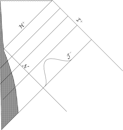
Figure 1: The physical setup for the scattering problem. A star of mass $M$ has undergone spherically symmetric collapse to form a black hole. The ingoing null worldtube ${\cal N}$ lies outside the collapsing matter. The metric inside ${\cal N}$ (but outside the matter) is vacuum Schwarzschild. Outside of ${\cal N}$, data for an ingoing pulse is specified on the initial outgoing null hypersurface ${\cal J}^{-}$. As the pulse propagates to the black hole event horizon ${\cal H}^{+}$, part of its energy is scattered to ${\cal I}^{+}$.

In Sec. II, we briefly summarize the characteristic formalism on which the paper is based. In Sec. III, we give the geometrical setup for initializing and setting boundary conditions for the simulations. In Sec. IV, we calibrate the accuracy of the full nonlinear code against results obtained with independent linearized characteristic codes Campanelli et al. (2001); Husa et al. (2002) that solve the Teukolsky equations Teukolsky (1972, 1973) for perturbations about Schwarzschild spacetime. We show, in the regime where linear perturbation theory is valid, that the full nonlinear code reproduces the Bondi news function obtained from the perturbative codes to second order accuracy.

Simulations of nonlinear mode-mode coupling are described in Sec. V. The nonlinear effects on the waveform of the outgoing radiation can be cleanly separated out by comparison with the waveform produced by the linearized code. The simulations reveal several nonlinear features of the waveform that have potential importance to the design of templates for data analysis. These are summarized in Sec. VI.

II The nonlinear scattering problem

Following Bishop et al. (1996, 1997); Gómez (2001); Gomez et al. (2002), we use coordinates based upon a family of outgoing null hypersurfaces, letting $u$ label these hypersurfaces, $x^{A}$ $(A=2,3)$, label the null rays, and $r$ be a surface area coordinate, such that in the $x^{\alpha}=(u,r,x^{A})$ coordinates the metric takes the Bondi-Sachs form Bondi et al. (1962); Sachs (1962)

$$ds^{2} = -\left[e^{2\beta}\left(1+{W\over r}\right)-r^{2}h_{AB}U^{A}U^{B}\right]du^{2}-2e^{2\beta}dudr$$ (1)

$$- 2r^{2}h_{AB}U^{B}dudx^{A}+r^{2}h_{AB}dx^{A}dx^{B}.$$

Here $W$ is related to the Bondi-Sachs variable $V$ by $V=r+W$ and $det(h_{AB})=det(q_{AB})$, with $q_{AB}$ a standard unit sphere metric. We represent $q_{AB}$ in terms of a complex dyad $q_{A}$ satisfying $q^{A}q_{A}=0$, $q^{A}\bar{q}_{A}=2$, $q^{A}=q^{AB}q_{B}$, with $q^{AB}q_{BC}=\delta^{A}_{C}$ and $q_{AB}=\frac{1}{2}\left(q_{A}\bar{q}_{B}+\bar{q}_{A}q_{B}\right)$. The angular coordinates $x^{A}=(q,p)$ used in the code are based upon a complex stereographic coordinate $z=q+ip$ for the unit sphere metric

$$q_{AB}dx^{A}dx^{B}=\frac{4}{1+q^{2}+p^{2}}(dq^{2}+dp^{2}),$$

with two patches used to cover the sphere. In the north patch, the stereographic coordinate is related to standard spherical coordinates $(\theta,\phi)$ by $z_{N}=\tan\frac{\theta}{2}e^{i\phi}$ (see App. A).

We represent tensors on the sphere by spin-weighted variables Gómez et al. (1996). Thus the conformal metric $h_{AB}$ is represented by the complex function $J=\frac{1}{2}h_{AB}q^{A}q^{B}$, and the real function $K=\frac{1}{2}h_{AB}q^{A}\bar{q}^{B}$, where $K^{2}=1+J\bar{J}$ on account of the condition $\det(h_{AB})=\det(q_{AB})$. The metric functions $U^{A}$ are similarly encoded in the complex function $U=q_{A}U^{A}$ Bishop et al. (1996, 1997). Angular derivatives are expressed in terms of $\eth$ and $\bar{\eth}$ operators. A brief description, along with our conventions for spin-weighted spherical harmonics, is given in App. A. For details, see Ref. Gómez et al. (1996).

The vacuum Einstein equations form (i) a hierarchy of null hypersurface equations for the radial derivatives of $\beta$, $U$ and $W$ (and also for auxiliary variables $\nu$, $k$, $B$ and $Q$ used to reduce the equations to first order differential form in the angular coordinates), (ii) a complex evolution equation for the metric function $J$ and (iii) a set of subsidiary equations which are satisfied by virtue of the other equations if they are satisfied on a null or timelike worldtube. In our case, a null worldtube forms the inner boundary of the computational domain, and we solve the equations induced there in the form discussed in Ref. Gomez et al. (2001). Most of the discussion in the present paper will deal with an “ingoing”pulse, in which case Schwarzschild data are posed on the inner boundary, the subsidiary equations are then solved automatically. The explicit form of the equations (i) and (ii) is given in Eq’s. (16)–(26) of Ref. Gómez (2001).

Given initial data $J$ on an outgoing null hypersurface extending to ${\cal I}^{+}$ and boundary data on an inner timelike or null world tube, the PITT null code carries out the future evolution of the spacetime. The evolution extends to ${\cal I}^{+}$ where the Bondi news function $N$ is calculated. In the present work, the computation of the news is carried out with enhanced accuracy by the new method described in App. B.

III Data for the scattering problem

The nonlinear simulations described in Sec. V model the scattering of an ingoing pulse in the region exterior to a spherically symmetric collapsing star of mass $M$, as depicted in Fig. 1 (the mass $M$ will always be scaled to 1 in our simulations). The free initial data for the pulse consist of the metric function $J$ on the initial outgoing null hypersurface, denoted by ${\cal J}^{-}$. In addition, Schwarzschild null data is given on the interior null hypersurface ${\cal N}$, which is causally unaffected by the pulse. The evolution code then provides the news function at ${\cal I}^{+}$. For computational simplicity, we simulate a mathematically equivalent problem by considering the Kruskal continuation of the Schwarzschild interior so that the inner boundary is extended to the ingoing branch of the $r=2M$ null hypersurface, which we denote by ${\cal H}^{-}$. In our metric ansatz (1) Schwarzschild data on ${\cal H}^{-}$ correspond to setting $\beta=0$, $U=0$, $W=-2M$. A schematic view of this setup, in the linear regime, is provided in Fig. 5 (Fig. 5 shows the compactified exterior Kruskal quadrant which includes ${\cal I}^{-}$ as well as ${\cal I}^{+}$). In the nonlinear simulations, the data on ${\cal H}^{-}$ is set to the Schwarzschild data $J=0$, which implies that the intended Schwarzschild data is also induced on ${\cal N}$. In the code calibration tests considered in Sec. IV we also consider outgoing pulses generated by data on ${\cal H}^{-}$.

We used two different types of evolution coordinates, $u$ and $\hat{u}$. For the calibration runs we chose as our evolution coordinate $u$ which is an affine parameter along the null generators of ${\cal H}^{-}$. For the remaining runs we chose as our evolution coordinate $\hat{u}$ which is the standard Schwarzschild retarded time on ${\cal H}^{-}$ ($\hat{u}=t-r^{*}$). Later, when analyzing gravitational wave signals, we will use Bondi time – an affine parameter $\tilde{u}$ along the null generators of ${\cal I}^{+}$. For Schwarzschild, Bondi time coincides with the standard Schwarzschild retarded time $\tilde{u}=\hat{u}$, and $u=-Mexp(-\tilde{u}/4M)$.

We prescribe the input data for the pulse in the form $J=f(x)\,{}_{2}R_{\ell\,m}$, where $x=r$ for initial data on ${\cal J}^{-}$ or $x=u$ for data on ${\cal H}^{-}$ and ${}_{s}R_{\ell\,m}$ are spin-weighted spherical harmonics with real potentials (see App. A). The ${}_{s}R_{\ell\,m}$ are linear combinations of the standard ${}_{s}Y_{\ell\,m}$ and form a complete basis for smooth spin-weight $s$ functions. In linear theory a particular ${}_{2}R_{\ell\,m}$ mode in the data produces a Bondi news function that contains only that mode. Conversely, data constructed from the standard spin-weighted spherical harmonics ${}_{2}Y_{\ell\,m}$ would produce both the ${}_{2}Y_{\ell\,m}$ and ${}_{2}Y_{\ell\,-m}$ modes in the Bondi news. An explanation for this linear mode-coupling and explicit formulae for the ${}_{s}R_{\ell\,m}$ are given in App. A.

The function $f$ determines the radial profile of the pulse. As for its initial angular dependence, we restrict our attention here to input data with $\ell=2$ and $m=0$ or $m=2$. In the regime where the linear approximation is valid, the Bondi news function $N$ will also be of this form but nonlinear effects lead to the presence of higher order modes. Parity and reflection symmetry implies that only even $\ell$ and even $m\geq 0$ modes be generated by such nonlinear effects.

The input pulse is specified in terms of the function

$$f(x)=A\frac{2^{2n}(x-x_{min})^{n}(x_{max}-x)^{n}}{(x_{max}-x_{min})^{2n}}$$ (2)

where $A$ controls the amplitude and $n$ controls the steepness. For outgoing pulses, we prescribe boundary data on ${\cal H}^{-}$ with the specific profile

$$J|_{{\cal H}^{-}}(u,x^{A})=f(u)\,{}_{2}R_{2\,m},$$ (3)

with $n=6$, for $u_{min}<u<u_{max}$; elsewhere we set $J=0$. For an ingoing pulse, we give data on the initial outgoing null hypersurface of the form

$$J(r,x^{A})=f(x)\,{}_{2}R_{2\,m}$$ (4)

for $x_{min}<x<x_{max}$, where $x=r/(2M+r)$, with either $n=3$ or $n=6$; elsewhere we set $J=0$. We also set $J=0$ on the inner boundary ${\cal H}^{-}$.

IV Calibration of the nonlinear code against perturbative solutions

We calibrate the Bondi news function obtained from the PITT nonlinear code against values obtained from a characteristic perturbative code Campanelli et al. (2001); Husa et al. (2002) based upon the Teukolsky equations for the Newman-Penrose quantities Newman and Penrose (1962) $\tilde{\psi}_{0}=C_{abcd}\tilde{l}^{a}m^{b}\tilde{l}^{c}m^{d}$ and $\tilde{\psi}_{4}=C_{abcd}\tilde{n}^{a}\bar{m}^{b}\tilde{n}^{c}\bar{m}^{d}$.

We fix the null tetrad by setting $\tilde{l}_{a}=-\nabla_{a}\tilde{u}$ and $m^{a}=q^{a}/\sqrt{2}r$, where $\tilde{u}=t-r^{*}$ in the background Schwarzschild spacetime [$r^{*}=r+2M\log(r/2M-1)$ is the Regge-Wheeler tortoise coordinate]. Rather than evolving the spin-weighted quantities $\tilde{\psi}_{0}$ and $\tilde{\psi}_{4}$, we evolve equivalent spin-zero potentials (see App. A) rescaled by appropriate factors of $r$. These evolution variables are $\tilde{F}_{4}$, where $\bar{\eth}^{2}\tilde{F}_{4}=r\tilde{\psi}_{4}$, and $\hat{F}_{0}$, where $\eth^{2}\hat{F}_{0}=(1-2M/r)^{2}r^{5}\tilde{\psi}_{0}$. Both $\tilde{F}_{4}$ and $\hat{F}_{0}$ are constructed to be finite on ${\cal I}^{+}$.

The perturbative variable $\tilde{F}_{4}$ has a complicated dependence on the Bondi metric variables. However, on ${\cal H}^{-}$, where the data for the outgoing pulse is prescribed, the expression for $\tilde{F}_{4}$ reduces to

$$\tilde{F}_{4}=\frac{u^{2}}{16M}\bar{j}_{,uu},$$ (5)

where $u=-M\exp(-\tilde{u}/4M)$ is an affine parameter along the null generators of ${\cal H}^{-}$ and $j$ is the spin-zero potential for $J$, i.e. $J=\eth^{2}j$. On an outgoing null hypersurface, where the data for an ingoing pulse is prescribed, the perturbative variable $\hat{F}_{0}$ has the simple dependence on $j$ given by

$$\hat{F}_{0}=\frac{1}{2}r(r-2M)^{2}\partial_{r}(r^{2}\partial_{r}j).$$ (6)

For input data consisting of an outgoing pulse, where we specify compact support boundary data for $J$ on ${\cal H}^{-}$ and set $J=0$ on ${\cal J}^{-}$, we directly obtain equivalent boundary data for $\tilde{F}_{4}$ via Eq. (5). For input consisting of an ingoing pulse, where we specify the compact support data on ${\cal J}^{-}$, we directly obtain the equivalent boundary data for $\hat{F}_{0}$ via Eq. (6). For the calibration tests presented here we choose input data with ($\ell=2$, $m=0$) spherical harmonic dependence for which $\tilde{F}_{4}=f_{4}(u,r)R_{2\,0}$ [$R_{\ell\,m}={}_{0}R_{\ell\,m}$] and $\hat{F}_{0}=f_{0}(u,r)R_{2\,0}$. The perturbative code provides solutions for $f_{4}$ and $f_{0}$. Details of the evolution code for $f_{4}$ can be found in Campanelli et al. (2001); and details for $f_{0}$, in Husa et al. (2002).

In the perturbative approach, the Bondi news function is either obtained directly from $\tilde{F}_{4}$ on ${\cal I}^{+}$ or indirectly from $\hat{F}_{0}$ Husa et al. (2002). The Bondi news function is given by

$$\bar{N}(\tilde{u})=\bar{\eth}^{2}\int_{-\infty}^{\tilde{u}}\tilde{F}_{4}|_{{\cal I}^{+}}(\tilde{t})d\tilde{t},$$ (7)

where the integral in Eq. (7) is over Bondi time. In the simulation of an outgoing pulse, the input data for $\tilde{F}_{4}$ on ${\cal H}^{-}$ is set to zero until the start of the evolution at $\tilde{u}=\tilde{u}_{min}$. In this case we calculate the Bondi news through a second-order accurate midpoint-rule integration of $\tilde{F}_{4}$.

In the simulation of the scattering of an ingoing pulse, the computation of the news function is more complicated. For the present case of an ($\ell=2$, $m=0$) linearized mode, the news function is related to $\hat{F}_{0}$ by

$$N+\frac{M}{2}\partial_{\tilde{u}}N=\frac{1}{6}\eth^{2}\partial_{\tilde{u}}^{3}\hat{F}_{0}|_{{\cal I}^{+}}.$$ (8)

Care must be taken in initiating the integration of Eq. (8) because the Bondi news function $N$ does not vanish at the initial evolution time. We need an accurate initial value for $N$, which we obtain by integrating Eq. (6) to obtain the metric variable $J$. In the linear regime, the Bondi news function can be calculated from the value of $J$ and its radial derivative at ${\cal I}^{+}$ Bishop et al. (1997). In the present case of an ($\ell=2$, $m=0$) linearized mode,

$$N=-\frac{1}{2}\left(3J+r^{2}\partial_{r}\partial_{\tilde{u}}J\right)|_{{\cal I}^{+}}$$ (9)

(a generic formula for the linearized News as a function of $J|_{\cal I}^{+}$ is given in Eq. (11)). We use Eq. (9) to obtain the news function on the initial slice and also to compute it at later times as a check that it produces the same values as the integration of (8).

Because the perturbative code is one-dimensional, computations on very large radial grids can be carried out to provide effectively exact solutions for calibrating the error in the Bondi news function calculated using the nonlinear code. Such a check must be carried out in the range of validity of the linear approximation, and the error in the perturbative calculation must be sufficiently smaller than the discretization error of the nonlinear null code. For this purpose, simulations with the perturbative code were carried out with 16001 radial grid points for the outgoing pulse. For the ingoing pulses (for which the perturbative code is less accurate), we used 2501, 5001, and 10001 radial grid points, and then performed a Richardson extrapolation to obtain high accuracy.

The initial and boundary data given by Eq’s. (3) and (4) are compact pulses with relatively steep profiles, which require comparatively large grid sizes to attain good resolution. The specific form of the profiles lead to $C^{3}$ differentiability of the associated perturbative quantities $\tilde{F}_{4}$ and $\hat{F}_{0}$, a requirement which ensures that the news function can be obtained from the perturbative calculation to second order accuracy. In all tests we scale the initial mass of the system to $M=1$.

IV.1 Propagation of outgoing pulses

In our first battery of tests, which provide stringent tests of the ability of the code to carry radiation away from the horizon ${\cal H}^{-}$ to null infinity ${\cal I}^{+}$, we prescribe an arbitrary perturbation on the horizon while setting the perturbation of the initial outgoing null cone to zero. The horizon data for $J$ are given by Eq. (3) with $u_{min}=-1.99$, $u_{max}=-1.5$, and $A=2.6\cdot 10^{-5}$. This corresponds to a relatively short pulse of $\Delta\tilde{u}\approx 1.13M$ in the background Schwarzschild retarded time. The corresponding data for $\tilde{F}_{4}$ are obtained by applying Eq. (5) to Eq. (3). We measure the error in the Bondi news function $N_{code}$ with the $L_{\infty}$ norm $\|N_{code}-N_{pert}\|_{\infty}$ restricted to the interior of the equator on the stereographic patches. Our primary concern is to check convergence and the evolution was stopped at $u=-1.5$ when the horizon data vanishes. The perturbative news function was obtained using $16001$ radial grid points and an initial time-step of $du=8\cdot 10^{-5}$.

The nonlinear characteristic code uses a uniform radial grid of $n_{x}$ points on the compactified coordinate $x=r/(R+r)$, where $R=2M$ is the initial horizon radius. The coordinate range is $1/2<x<1$, with $x=1/2$ at ${\cal H}^{-}$ and $x=1$ at ${\cal I}^{+}$. We introduce two additional ghost zones inside the horizon in accord with the start-up algorithm described in Gomez et al. (2002). The angular grid is also uniform, with $n_{q}$ grid points spanning the range $(-q_{S},q_{S})$ in both the $q$ and $p$ directions. We set $q_{S}=1.2$ in order to provide a finite overlap between the two stereographic patches. In the convergence tests we take $n_{q}=12i+5$, $n_{x}=30i+3$, with $i$ taking integer values from 6 to 11. We keep the time step $du$ constant during each run, at $du=5.6\cdot 10^{-3}/i$, below the smallest value required for the CFL condition to be satisfied and scaling with $i$ to guarantee convergence.

Since the code is second order accurate, and the linear approximation holds, the error norm should be inversely proportional to the square of the grid size, i.e. to $i^{2}$. Figure 2 shows the rescaled $L_{\infty}$ norm of the error for the above 6 grids.

Figure 2: The rescaled $L_{\infty}$ norms ${\cal E}=(i/6)^{2}\|N_{code}-N_{pert}\|_{\infty}$ (versus time) of the Bondi news for the compact support outgoing pulse.

Note the perfect overlap at early times (prior to $u=-1.65$). The later errors scale approximately with $i^{2}$ but show definite deviations. Runs with smaller amplitude indicate that this error is not a nonlinear effect. The error appears to be due to accumulation of higher order truncation error, mixed with some smaller roundoff error. Nevertheless, the calculation is still extremely accurate including up to the end of the run, when deviation from strict second order convergence is more noticeable. This is evident from Fig. 3, which shows the news function and the $L_{\infty}$ error norm (multiplied by $2000$) for the finest grid. The error is at least 200 times smaller than the news function; thus controlled errors of less than one-half of a percent are achievable at the larger resolutions.

Figure 3: The news and $L_{\infty}$ norm ${\cal E}=\|N_{code}-N_{pert}\|_{\infty}$ (rescaled by a factor of 2000) for the compact support outgoing pulse.

IV.2 Scattering of ingoing pulses

These tests correspond to the realistic situation of the scattering of gravitational radiation which has been created in the near field of a black hole. We place a compact support pulse on the initial null hypersurface and set the boundary data on ${\cal H}^{-}$ to zero. The initial data were given by Eq. (4). The setup is described in Fig. 1. The perturbation calculation was carried out using the evolution algorithm for $\hat{F}_{0}$ described in Husa et al. (2002). For this test we choose $x_{min}=0.6$, $x_{max}=0.8$, $n=6$, and an amplitude $A$ of $2.6\cdot 10^{-6}$. The corresponding pulse initially extends from $r=3M$ to $r=8M$. The nonlinear runs were performed with the same grid parameters as in Sec. IV.1, with the grid sizes again determined by the integer $i$ ranging from 6 to 11. The time step was set to $du=-u\,5\cdot 10^{-4}/i$, where the factor of $u$ ensures that the CFL condition remains satisfied (by approximately a factor of 1/4). Figure 4 shows the rescaled $L_{2}$ norm of the error ${\cal E}=(i/6)^{2}\|N_{code}-N_{pert}\|_{2}$ for the above 6 grids. The excellent overlap of the norms confirms that the nonlinear null code is second order convergent.

The second order convergence of the news from the ingoing pulse begins to break down at $\tilde{u}=15M$ as a consequence of our choice of coordinate system. Fig. 5 shows a plot of Schwarzschild background spacetime with the timelike curves corresponding to the worldlines of the first few radial gridpoint (the ingoing null curve ${\cal H}^{-}$ is the innermost gridpoint). An initially compact pulse, bounded by the ingoing null lines ${\cal K}_{1}$ and ${\cal K}_{2}$, is placed on ${\cal J}^{-}$. At the time level ${\cal J}^{+}$ the ingoing pulse will occupy a region containing only a few radial gridpoints. Consequently, a well resolved pulse on the initial slice will cease to be resolved in a finite amount of time. Radial resolution of the ingoing pulse begins to break down at $\tilde{u}=15M$. This breakdown in resolution happens relatively quickly because we chose a grid that is uniform in the $x$ coordinate. The evolutions could be extended by using adaptive mesh refinement techniques recently developed for characteristic codes Pretorius and Lehner (2003), and by different choices for the compact radial coordinate. (Note that the loss of resolution happens in the radial direction, not in the angular ones, so that the techniques in Pretorius and Lehner (2003) could be readily applied to this case. We will revisit this point in Sec. VI)

Figure 4: The rescaled $L_{2}$ norm ${\cal E}=(i/6)^{2}\|N_{code}-N_{pert}\|_{2}$ versus grid-parameter $i$ for the ingoing pulse test. Second order convergence is confirmed by the reasonable overlap of the norms.

Figure 5: The ingoing pulse on a Schwarzschild background. The timelike curves (along with ${\cal H}^{-}$) are the worldlines of the first 5 radial gridpoints (the first gridpoint is located at ${\cal H}^{-}$). The $r=const$ lines begin at past timelike infinity $i^{-}$ and terminate at future timelike infinity $i^{+}$. An ingoing pulse well resolved on ${\cal J}^{-}$ is compressed (in the $x$ coordinate) into 3 gridpoints by the time it reaches ${\cal J}^{+}$

V Analysis of mode-mode coupling in gravitational radiation scattering

The $(u,x,x^{A})$ coordinates, which define the computational grid of the PITT code Bishop et al. (1997); Gómez (2001) are adapted to the geometry of the inner boundary. A gravitational wave detector would measure the radiation as seen in a distant inertial coordinate system, located essentially at ${\cal I}^{+}$. We denote by $(u_{B},y^{A})$ the corresponding inertial Bondi coordinates on ${\cal I}^{+}$ (where $x=1$). Thus for the purposes of gravitational wave data analysis the news function must be expressed in the form $N(u_{B},y^{A})$. In the course of this work, modules have been added to the PITT code to carry out this transformation, which is essential in order to provide correct time profiles and harmonic mode analysis. In the linear regime, $(u,x^{A})\approx(u_{B},y^{A})$ so that these corrections to the news function are of second order and can be ignored. That is no longer the case when we consider the nonlinearities manifested by mode coupling.

The “inertial” news function $N(u_{B},y^{A})$ is obtained by performing a fourth order accurate interpolation between the $(u,x^{A})$ and $(u_{B},y^{A})$ grids. It is then decomposed into spin-weight 2 spherical harmonic amplitudes $N_{\ell\,m}$ via second order accurate integration over the sphere with solid angle $\Omega=4\pi$,

$$N_{\ell\,m}=\oint N\,{}_{2}\bar{R}_{\ell\,m}\,d\Omega.$$ (10)

See App. A for further details concerning the spin-weighted harmonic decomposition and how the integration is carried out on the stereographic patches.

In linear theory, in a gauge where $\beta=O(A^{2})$ and $U=O(A)$, the $N_{\ell\,m}$ coefficients are related to the $J_{\ell\,m}$ coefficients of the metric function $J$ (obtained by applying Eq. (10) to $J$ rather than $N$) by

$$N_{\ell\,m}=-\frac{1}{2}r^{2}\partial_{r}\partial_{u}J_{\ell\,m}-\frac{\ell(\ell+1)}{4}\Re{(J_{\ell\,m})}.$$ (11)

In linear theory there is no mode coupling in $J$, and initial data containing a single ${}_{2}R_{\ell\,m}$ mode produces a Bondi news function containing only that mode.

V.1 Axisymmetric mode coupling

We first study mode coupling in the axisymmetric case by prescribing initial data as an ingoing ($\ell=2$, $m=0$) pulse, as in Eq. (4) with $n=3$, $x_{min}=.56$, and $x_{max}=.8$. This choice of initial pulse, extending from $r=2.55M$ to $r=8M$, is made for computational economy because the nonlinear effects are weak for $r\gg 3M$. We vary the amplitude from $A=2.6\cdot 10^{-6}$, well in the linear regime, to $A=2.6\cdot 10^{-1}$, where nonlinear effects can be clearly observed. We display results obtained with a resolution of $77\times 77$ angular grid points and $181$ radial grid points. This grid size (the size of the base grid used in the convergence tests) allows a broad search for interesting qualitative behavior with reasonable computational time. The news function is computed in inertial Bondi coordinates and then decomposed into spin-weight 2 spherical harmonics. The reflection symmetry and axisymmetry of the initial data are preserved by the numerical evolution in the nonlinear regime, so that the only non-vanishing amplitudes $N_{\ell\,m}$ of the scattered radiation have even $\ell$ and $m=0$. In addition, these symmetries imply that the $N_{\ell\,0}$ are real, which in our conventions means that only the $\oplus$ polarization mode is excited.

The following figures show the time dependence of the lowest order mode amplitudes, $N_{2\,0}$, $N_{4\,0}$, and $N_{6\,0}$, which are excited in the news function by a given input amplitude $A$. Figure 6 shows the dependence of $N_{2\,0}/A$ on $A$. From the figure it is clear that nonlinear effects do not make $N_{2\,0}$ deviate significantly from its perturbative waveform for $A<2.6\cdot 10^{-2}$. However, at higher amplitudes the effect of nonlinearity is to amplify the wave, which could enhance the prospects of detection above the level predicted by linearized theory. This nonlinear amplification is primarily quadratic in $A$. In addition to the nonlinear amplification there is also a phase shift which can be seen more clearly in Fig. 11.

Nonlinear effects are more easily seen in the modes that vanish in the linearized approximation. Figure 7 shows that $N_{4\,0}$ scales as $A^{2}$ at sufficiently high amplitudes. For smaller amplitudes $A\,$ this quadratic scaling is masked by the truncation error introduced in the computation of the spherical harmonic decomposition of the news function at the given grid size and, as a result, $N_{4\,0}$ scales roughly linearly with $A$.

Figure 8 shows $N_{6\,0}$ scales as $A^{3}$ at the highest amplitudes. As might be expected for a higher $\ell$ mode, the masking effects of truncation error are now more severe at the lower amplitudes. The breakdown of scaling behavior in Fig’s. 6 - 8 results from inaccuracy at times beyond $\tilde{u}=20$ due to lack of resolution of short scale features using the current grid. These short scale features arise inside $r=3M$ where quasinormal ringing is known to originate.

Figure 6: The rescaled coefficient $N_{2\,0}/A$ for $A=2.6\cdot 10^{-1},2.6\cdot 10^{-1.2},2.6\cdot 10^{-1.5},2.6\cdot 10^{-2},\cdots,2.6\cdot 10^{-6}$. For $A<2.6\cdot 10^{-2}$, $N_{2\,0}/A$ has negligible dependence on $A$ and the curves overlap.

Figure 7: The rescaled coefficient $N_{4\,0}/A$ for $A=2.6\cdot 10^{-3},2.6\cdot 10^{-4},\cdots,2.6\cdot 10^{-6}$, and the rescaled coefficient $N_{4\,0}/A^{2}$ for $A=2.6\cdot 10^{-1},2.6\cdot 10^{-1.2},2.6\cdot 10^{-1.5},2.6\cdot 10^{-2}$. Note that at early times $N_{4\,0}/A$ is independent of $A$ for $A<2.6\cdot 10^{-4}$. For small $A$, the computed value of $N_{4\,0}$ is dominated by truncation error and is thus proportional to $A$. For larger $A$, where its computed value is of physical relevance, $N_{4\,0}$ is proportional to $A^{2}$. When $A=2.6\cdot 10^{-3}$, the coefficient contains a mixture of order $O(A)$ truncation error and order $O(A^{2})$ non linear terms.

Figure 8: The rescaled coefficient $N_{6\,0}/A$ for $A=2.6\cdot 10^{-2},\cdots,2.6\cdot 10^{-6}$, and the rescaled coefficient $N_{6\,0}/A^{3}$ for $A=2.6\cdot 10^{-1},2.6\cdot 10^{-1.2},2.6\cdot 10^{-1.5}$. Note that $N_{6\,0}/A$ is independent of $A$ for $A<2.6\cdot 10^{-2}$. For small $A$, the value of the $N_{6\,0}$ is dominated by truncation error and is thus proportional to $A$. For larger $A$, the coefficient is proportional to $A^{3}$. However, the nonlinear terms in $N_{6\,0}$ are smaller than truncation error for $A$ as large as $2.6\cdot 10^{-2}$.

There are some understandable aspects in these mode coupling results. Apart from numerical truncation error effects at low amplitudes, we find that the corresponding amplitudes $N_{\ell\,0}$ scale as $A^{\ell/2}$. This is consistent with the property of ordinary spherical harmonics

$$\left(Y_{\ell\,m}\right)^{j}\sim Y_{(j\ell)\,m}+\mbox{terms with smaller $\ell$}.$$

Thus we expect that an $\ell=2j$ mode arises from order $j$ (and higher) nonlinear terms, and hence will scale as $A^{j}+O(A^{j+1})$. The theory of how the Einstein equations couple these spin-weighted spherical harmonics has not been worked out. A full analysis of the possible modes produced at a given order would require a computation of the appropriate Clebsch-Gordon coefficients for spin-weighted spherical harmonics. Finding these coefficients is complicated by the fact that there are many ways to combine $\ell$ and $m$ modes of various spin-weights to produce a spin 2 function (e.g. ${}_{4}R_{\ell\,m}\,\,{}_{2}\bar{R}_{\ell^{\prime}\,m^{\prime}}$; ${}_{1}R_{\ell\,m}\,\,{}_{1}R_{\ell^{\prime}\,m^{\prime}}$; ${}_{0}R_{\ell\,m}\,\,{}_{2}R_{\ell^{\prime}\,m^{\prime}}$; $\cdots$). Rather than work out these coefficients we use a more naive approach of looking at the possible modes produced by combinations of spin-weight 0 harmonics. From this approach we find that the possible modes produced by combining an ($\ell=2$, $m=0$) mode with itself (i.e. quadratic coupling) are ($\ell=4$, $m=0$) and ($\ell=2$, $m=0$) [$\ell=0$ is not allowed for spin 2 fields]. Thus the ($\ell=2$, $m=0$) mode in the news would contain linear and higher order terms, whereas the ($\ell=4$, $m=0$) mode would contain quadratic and higher terms. The above numerical results are consistent with these naive expectations. In addition, there is a similar behavior in the frequencies of the various $\ell$ modes. Figure 9 shows the Fourier transforms of the $N_{2\,0}$, $N_{4\,0}$, and $N_{6\,0}$ coefficients for the $A=2.6\cdot 10^{-1}$ run. The ($\ell=2$, $m=0$) mode shows a strong peak with maximum at $\omega\approx.36$; the ($\ell=4$, $m=0$) mode has peaks at $\omega\approx.73$ and $\omega\approx 0$; and the ($\ell=6$, $m=0$) mode has peaks at $\omega\approx 1.10$ and $\omega\approx.30$. This entire behavior is exactly what would arise from the nonlinear power law response $f^{\ell/2}$ to an $\ell=2$ mode $f$; i.e. quadratic terms produced from $f\sim\sin\omega_{0}t$ contains frequencies $2\omega_{0}$ and $0$. Similarly, cubic terms produce frequencies $\omega_{0}$ and $3\omega_{0}$.

The dominant contribution to the frequency of the ($\ell=2$, $m=0$) mode is expected to be the lowest $\ell=2$ quasinormal frequency. For an $M=1$ black hole the lowest $\ell=2$ quasinormal frequency is $\omega=.373672$ Nollert and Schmidt (1992). However, the $A=2.6\cdot 10^{-1}$ amplitude pulse should contribute significant mass to the system and a lower frequency should be expected, in agreement with the measured peak at $\omega\approx.36$. To measure the accuracy of the frequencies obtained for these systems we performed a similar analysis with the $A=2.6\cdot 10^{-6}$ run. In this low amplitude limit, the Fourier transform of $N_{2\,0}$ showed a maximum at $\omega\approx.37$, very close to the frequency of the lowest quasinormal mode.

Figure 9: Fourier transforms (after rescaling to similar amplitudes to facilitate comparison of peak locations) of the $N_{2\,0}$, $N_{4\,0}$, and $N_{6\,0}$ time profiles for the $A=2.6\cdot 10^{-1}$ run. The ($\ell=2$, $m=0$) mode shows a strong peak at $\omega\approx.36$, the ($\ell=4$, $m=0$) mode shows a strong peak at $\omega\approx.73$ and $\omega\approx 0$, and the ($\ell=6$, $m=0$) mode shows a strong peak at $\omega\approx 1.10$ and $\omega\approx.30$.

Of direct importance for designing templates for wave detection is the waveform obtained by the net superposition of these modes. In Fig. 10 we plot the time dependence of the inertial news function, as measured by an observer at the equator in a coordinate system adapted to ${\cal I}^{+}$, as a function of input amplitude. The figure shows nonlinear amplification of the news function with increasing input amplitude. The peaks of the waveform differ by up to a factor of 2 from the values which would be obtained by a linearized calculation.

In addition there are phase shifts in the location of the peaks. These are apparent in Fig. 11 which compares $N/A$ at the equator for the nonlinear case $A=2.6\cdot 10^{-1}$ and the linear case $A=2.6\cdot 10^{-6}$. The difference between these two waveforms corresponds to the error that would be made by using a linearized calculation to obtain the $A=2.6\cdot 10^{-1}$ waveform. In the first oscillation the $A=2.6\cdot 10^{-1}$ run has the larger wavelength, while afterward its wavelength is shorter.

Accurate knowledge of the phase is very important to data analysis for extracting the signal Cutler et al. (1993). When using matched filtering over a number of cycles of the waveform, the total integrated error in the phase must be no greater than 10% of a cycle. For example, a phase shift of 2% per cycle from the value programmed into the detection template would render the phase information useless in 5 cycles. The trend displayed in Fig’s. 10 and 11 is a drift in phase of about 15% from the first maximum to the first minimum. The nonlinear news oscillates quicker in this first half cycle. This trend is reversed in the second half of the first cycle and the net phase shift relative to the linear news after the first complete cycle is $2\%$. Beyond the first cycle the nonlinear news exhibits a consistently shorter oscillation period than the linear news. These results are of potential importance but, as already cautioned, at the current resolution it is not clear how accurate they are past $\tilde{u}\approx 20$.

Figure 10: The rescaled Bondi news function $N/A$ on the equator. The plot is very similar to Fig. 6 (the plots differ by an overall factor which results from the normalization of ${}_{2}R_{2\,0}$ and phase shifting in the larger amplitude runs) due to the dominance of the ($\ell=2$, $m=0$) mode. The news is axisymmetric and contains only the $\oplus$ mode.

Figure 11: The news measured by an observer on the equator for $A=2.6\cdot 10^{-1}$ and $A=2.6\cdot 10^{-6}$. The amplitudes have been rescaled by a factor $\sim 1/A$ to make comparison of the waveforms easier.

V.2 Azimuthal mode coupling

We study azimuthal effects of mode coupling by prescribing initial data as an ingoing ${}_{2}R_{2\,2}$ pulse. Again we give the data in the form of Eq. (4) with $n=3$, $x_{min}=.56$, and $x_{max}=.8$, we vary the amplitude from $A=10^{-6}$ to $A=.36$ and we use a fixed grid of $77\times 77$ angular grid points and $181$ radial grid points (larger grids are used when analyzing the cubic modes). The parity and reflection symmetries of the initial data are preserved by the nonlinear evolution, so that the only non-vanishing amplitudes $N_{\ell\,m}$ of the scattered radiation have even values of $\ell$ and even $m\geq 0$. However, in this case, both the $\oplus$ and $\otimes$ polarization modes are excited. We decompose the resulting news function in terms of the spin-weighted functions ${}_{2}R_{\ell\,m}$ up to $\ell=6$. The non-vanishing quadratic modes present in the news were the ${}_{2}R_{2\,0}$, ${}_{2}R_{4\,0}$, and ${}_{2}R_{4\,4}$ harmonics. The non-vanishing cubic modes were the ${}_{2}R_{4\,2}$, ${}_{2}R_{6\,2}$ and ${}_{2}R_{6\,6}$ harmonics.

Fig. 12 shows the coefficient $N_{2\,2}/A$ versus $A$. In linear theory the dependence of $N_{2\,2}$ on $A$ is linear, and this is observed for the entire run when $A\leq.1$. Nonlinear amplification and phase shifts are only apparent for $A=.36$.

Figure 12: Azimuthal coupling. The rescaled coefficient $N_{2\,2}/A$ is plotted versus time. Note the near perfect linear dependence of $N_{2\,2}$ on $A$ for $A\leq.1$. Nonlinear effects are only evident for the largest amplitude.

Fig’s. 13, 14, and 15 graph the coefficients $N_{2\,0}/A^{2}$, $N_{4\,0}/A^{2}$, and $N_{4\,4}/A^{2}$ respectively. In each case there is a near perfect early time overlap between the curves at different amplitudes for $A\leq.1$. These nonlinear modes exhibit a quadratic dependence on $A$ except for a late time amplification of the $A=.36$ curves in all modes and a late time amplification of the $A=.1$ curve of the $N_{4\,0}$ mode. This late time amplification results from cubic and higher terms contributing to the modes. The very strong late-time behavior observed in $N_{4\,0}$ may result from the loss of resolution near $r=2M$.

Figures 16, 17, and 18 graph the coefficients $N_{4\,2}/A^{3}$, $N_{6\,2}/A^{3}$, and $N_{6\,6}/A^{3}$. These modes show a cubic dependence on $A$, and were obtained by using a computational grid of $137\times 137$ angular gridpoints and $331$ radial gridpoints (roughly twice the resolution of the previous runs). The amplitudes for these runs were $A=.20$, $A=.26$, and $A=.36$.

The early time behavior of the ($\ell=2$, $m=0$) mode, unlike the behavior of the other nonlinear modes, is dominated by a low frequency component. However, hidden in this large signal is a higher frequency signal with roughly twice the frequency of the ($\ell=2$, $m=2$) mode. Fig. 19 shows the Fourier decomposition for these modes. The ($\ell=2$, $m=2$) mode has a strong peak at $\omega\approx.33$, the ($\ell=2$, $m=0$) mode has strong peaks at $\omega\approx.80$ and $\omega\approx.18$, and both the ($\ell=4$, $m=0$) and the ($\ell=4$, $m=4$) modes have strong peaks at $\omega\approx.70$. Given the large widths of the peaks, they are roughly consistent with the expected behavior of modes generated by quadratic response to an ($\ell=2$, $m=0$) mode. On the other hand the frequency spectrum of the ($\ell=4$, $m=2$) mode has a maximum at $\omega\approx.63$. The expected frequency of a cubic mode is either the frequency of the principal mode or three times the principal frequency. This drift toward larger than expected frequencies mirrors the behavior of the ($\ell=2$, $m=0$) mode. The ($\ell=6$, $m=2$) mode has a maximum at $\omega\approx 1.23$ while the ($\ell=6$, $m=6$) mode has a maximum at $\omega\approx 1.02$. These latter two results are roughly consistent with the expected behavior for cubic modes.

Figure 13: Azimuthal coupling. The rescaled coefficient $N_{2\,0}/A^{2}$ is plotted versus time. Note the near perfect quadratic dependence of $N_{2\,0}$ on $A$ for $A\leq.1$. Hidden within the low frequency signal at $\tilde{u}<15$ there is a higher frequency mode as is apparent in Fig. 19. The slight deviation of the $A=10^{-6}$ curve is due to roundoff error.

Figure 14: Azimuthal coupling: The rescaled coefficient $N_{4\,0}/A^{2}$ is plotted versus time. Note the near perfect quadratic dependence of $N_{4\,0}$ on $A$ at early times. The late-time deviation of the $A=.36$ curve may be due to the loss of resolution near $r=2M$. The frequency is roughly twice that of $N_{2\,2}$.

Figure 15: Azimuthal coupling: The rescaled coefficient $N_{4\,4}/A^{2}$ is plotted versus time. Note the near perfect quadratic dependence of $N_{4\,4}$ on $A$ for $A\leq.1$. The late time deviation is only significant for $A\geq.1$. The frequency is roughly twice that of $N_{2\,2}$.

Figure 16: Azimuthal coupling: The rescaled coefficient $N_{4\,2}/A^{3}$ is plotted versus time. The overlap of the curves is reasonably good, but the frequency does not correspond to the expected behavior for a cubic mode.

Figure 17: Azimuthal coupling: The rescaled coefficient $N_{6\,2}/A^{3}$ is plotted versus time. The overlap of the curves is reasonably good. Tests with higher resolution ($269\times 269$ angular gridpoints) indicate that the poor early time scaling is due to truncation error. The frequency is roughly three times that of the $N_{2\,2}$ mode.

Figure 18: Azimuthal coupling: The rescaled coefficient $N_{6\,6}/A^{3}$ is plotted versus time. The overlap of the curves is reasonably good. The frequency is roughly three times that of the $N_{2\,2}$ mode.

Figure 19: Azimuthal coupling, The Fourier response (absolute value) to an $A=.36$ pulse is shown for the first few modes. The Fourier integrals were restricted to $\tilde{u}<15$ and the resulting functions were rescaled to all have similar sizes. The dominant frequency of the $N_{2\,2}$ mode is $\omega\approx.33$. The $N_{2\,0}$ mode shows a strong low frequency peak at $\omega\approx.18$ and a weaker peak at $\omega\approx.80$. Interestingly, the transforms of $N_{4\,0}$ and $N_{4\,4}$ are very similar with both having strong peaks at $\omega\approx.70$. The $N_{4\,2}$ mode (a cubic mode) shows an unexpected strong peak at $\omega\approx.63$. The $N_{6\,2}$ mode shows a strong peak at $\omega\approx 1.23$ while the $N_{6\,6}$ mode has a strong peak at $\omega\approx 1.02$.

Fig. 20 shows the Bondi news observed at $q=p=.5$ ($\theta\simeq 70^{o},\phi=45^{o}$) for the $A=.36$, $A=10^{-1}$, and $A=10^{-6}$ non-axisymmetric runs. In the linearized approximation, the news in this angular direction is always imaginary, corresponding to pure $\otimes$ polarization. Nonlinear effects couple the $\oplus$ and $\otimes$ modes. Initial data with $A=.1$ produce a significant $\oplus$ component with amplitude roughly 28% of the $\otimes$ component; while initial data with $A=.36$ (at $\tilde{u}=20$) produces an $\oplus$ component 28% larger than the $\otimes$ component. Note that there is no significant nonlinear change in amplitude for the $\otimes$ component for $A\leq.1$. However, if a gravitational wave detector were not precisely oriented to measure the $\otimes$ component, significant nonlinear amplification and phase shifting would arise from the superposition of the $\oplus$ and $\otimes$ components. In the axisymmetric case, all of the gravitational radiation is in the $\oplus$ mode, and a gravitational wave detector would see the same nonlinear amplification and phase shifts regardless of orientation. In the present case the degree of nonlinear amplification and phase shifting depends on the orientation of the detector.

Figure 20: Azimuthal $\otimes$, $\oplus$ coupling. The news is shown in the $q=p=.5$ observation direction and has been rescaled by $1/A$. The rescaled $\otimes$ component of the $A=10^{-1}$ and $A=10^{-6}$ runs overlap. Nonlinear changes in amplitude and phase are visible in the $\otimes$ component of the $A=.36$ run.

We can gain insight into this problem by looking at the behavior of the real, spin-weight zero spherical harmonics $R_{\ell\,m}={}_{0}R_{\ell\,m}$ (in a similar way as done in Sec. V.1). For $m$ even and positive, $R_{\ell\,m}$ is reflection symmetric about the $q$ axis and has even parity with respect to the $(q,p)$ coordinate system. For $m$ even and negative, $R_{\ell\,m}$ has even parity but is reflection antisymmetric about the $q$ axis. Any product of positive, even $m$ harmonics will contain these two symmetries and is therefore a sum of even, positive $m$, real spherical harmonics. Along with the reflection symmetry of Einstein’s equations, this would seem to imply that data consisting of a positive, even $m$ harmonic with even $\ell$ would yield a Bondi news function consisting solely of positive, even $m$ and even $\ell$ harmonics. In addition, we can predict the possible modes generated by an ($\ell=2$, $m=2$) pulse and in what order they appear. For example, the quadratic modes produced by ($\ell=2$, $m=2$) initial data are ($\ell=2$, $m=0$), ($\ell=4$, $m=0$), and ($\ell=4$, $m=4$). Note that there is no quadratic ($\ell=2$, $m=2$) response. Thus quadratic terms in the Einstein equation do not affect the principal mode. Consequently there is no apparent nonlinear amplification or phase shift in this mode for $A\leq.1$ (see Fig. 12). Cubic terms can generate an ($\ell=2$, $m=2$) mode so we expect those terms to produce nonlinear amplification and phase shifts when they become significant.

V.3 Generating catalogs of waveforms

The results presented in Sec’s. V.1 and V.2 suggest a method for efficiently producing a catalog of waveforms produced by a given profile of the initial data with amplitude smaller than, say, $A=.1$. First perform a run with the linearized code to generate the linear part of the waveform. Then perform a single nonlinear run at an amplitude of $A=.1$. One then subtracts off the linear contribution to the various ($\ell$, $m$) modes and obtains the quadratic and cubic terms. The scaling with amplitude $A$ of each of the ($\ell$, $m$) modes can be determined by the arguments given in Sec’s. V.1 and V.2, and the net waveform for any $A\lesssim.1$ can be reconstructed.

For example, consider the waveform generated from an axisymmetric ($\ell=2$, $m=0$) input pulse with an amplitude $A=.1$. We first subtract off the linear part of the ($\ell=2$, $m=0$) profile to get the quadratic part of the ($\ell=2$, $m=0$) mode. We then assume a scaling of $A^{2}$ for this part of the ($\ell=2$, $m=0$) mode and the ($\ell=4$, $m=0$) mode, as well as a cubic scaling for the ($\ell=6$, $m=0$) mode. We can then produce the news for all $A\lesssim.1$ from a single nonlinear run.

VI Conclusion

We have shown how a characteristic code can be employed to investigate the nonlinear response of a black hole to the infall of gravitational wave energy. This problem, which is of importance to the observation and interpretation of gravitational waves, can in this way be studied with a mature, reliable evolution code. In this paper we have focused on the onset of nonlinear behavior in the waveform produced by the scattering of a pulse of radiation incident on a Schwarzschild black hole. However, given sufficient resolution, the same computational approach could be extended to many other scenarios, such as the waveform emitted by the dispersion of a pulse of radiation propagating approximately along the $r=3M$ (unstable) orbit about a Schwarzschild black hole, as we might expect from the gravitational perturbation associated with a bounded distribution of matter in such an orbit.

Besides the computation of accurate waveforms, our study reveals several features of qualitative importance:

• I. The mode coupling amplitudes consistently scale as powers $A^{n}$ of the input amplitude $A$ corresponding to the nonlinear order of the terms in the evolution equations which produce the mode. This allows much economy in producing a waveform catalog. Given the order $n$ associated with a given mode generation, the response to any input amplitude $A$ can be obtained from the response to a single reference amplitude $A_{0}$.

• II. The frequency response has similar behavior but in a less consistent way. The dominant frequencies produced by mode coupling are in the approximate range of the quasinormal frequency of the input mode and the expected sums and difference frequencies generated by the order of nonlinearity.

• III Large phase shifts, ranging up 15% in a half cycle relative to the linearized waveform, are exhibited in the news function obtained by the superposition of all output modes, i.e. in the waveform of observational significance. These phase shifts, which are important for design of signal extraction templates, arise in an erratic way from superposing modes with different oscillation frequencies. This furnishes another strong argument for going beyond the linearized approximation in designing a waveform catalog for signal extraction.

• IV Besides the nonlinear generation of harmonic modes absent in the initial data, there is also a stronger than linear generation of gravitational wave output. This provides a potential mechanism for enhancing the strength of the gravitational radiation produced during, say, the merger phase of a binary inspiral above the strength predicted in linearized theory.

• V In the non-axisymmetric case, there is also considerable generation of radiation in polarization states not present in the linearized approximation. In our simulations, input amplitudes in the range $A=.1$ to $A=.36$ lead to nonlinear generation of a $\oplus$ component which is of the same order of magnitude as the $\otimes$ component (which would be the sole component according to linearized theory). As a result, significant nonlinear amplification and phase shifting of the waveform can be observed depending on the orientation of a gravitational wave detector.

As already noted by Papadopoulos in his work on axisymmetric mode coupling Papadopoulos (2002), these effects arise from three types of nonlinearity: (i) Modification of the light cone structure governing the principal part of the equations and hence the propagation of signals; (ii) Modulation of the Schwarzschild potential by the introduction of an angular dependent “mass aspect”; and (iii) Quadratic and higher order terms in the evolution equations which couple the modes.

Although Papadopoulos studied nonlinear mode generation produced by an outgoing pulse, as opposed to the case of an ingoing pulse studied here, these same factors are in play and it is not surprising that both studies have common features. In both cases, the major nonlinear effects arise in the region near $r=3M$. Analogs of items I - IV above are all apparent in Papadopoulos’s results. At the finite difference level, both codes respect the reflection symmetry inherent in Einstein’s equations and exhibit the corresponding selection rules arising from parity considerations. In the axisymmetric case considered by Papadopoulos, this forbids the nonlinear generation of a $\oplus$ mode from a $\otimes$ mode, as in item V above.

The evolution along ingoing null hypersurfaces in the work of Papadopoulos and the evolution along outgoing null hypersurfaces in the present work have complementary numerical features. The grid based upon ingoing null hypersurfaces avoids the difficulty depicted in Fig. 5 in resolving effects close to $r=2M$ with a grid based upon outgoing null hypersurfaces. The outgoing code would require some form of mesh refinement in order to resolve the quasinormal ringdown for as many cycles as achieved by Papadopoulos. However, the outgoing code avoids the late time caustic formation noted in Papadopoulos’s work, as well as the gauge ambiguity and backscattering which complicate the extraction of waveforms on a finite worldtube. An attractive option is to combine the best features of both codes by matching an interior evolution based upon ingoing null hypersurfaces to an exterior evolution based upon outgoing null hypersurfaces, as implemented in Lehner (2000) for spherically symmetric Einstein-Klein-Gordon waves.

The waveform of relevance to gravitational wave astronomy is the superposition of modes with different frequency compositions and angular dependence. Although this waveform results from a complicated nonlinear processing of the input signal, which varies with choice of observation angle, we have shown that the response of the individual modes to an input signal of arbitrary amplitude can be obtained by scaling the response to an input of standard reference amplitude. This offers an economical approach to preparing a waveform catalog.

Work is in progress pursuing the above projects, as well as extending the treatment to spinning black holes. In concert with other approaches to compute nonlinear waveforms, it is hoped that robust features of the gravitational waves produced by highly distorted black holes will be discovered which could be exploited in data analysis efforts.

Appendix A Spin weighted spherical harmonics

The complex stereographic coordinate $z=q+ip$ covers the sphere with two patches which overlap in a region containing the equator. In the north patch, the stereographic coordinate is related to standard spherical coordinates $(\theta,\phi)$ by $z_{N}=\tan\frac{\theta}{2}e^{i\phi}$; and in the south patch, by $z_{S}=\cot\frac{\theta}{2}e^{-i\phi}$. In the overlap region, the coordinates are related by $z_{S}=1/z_{N}$.

In the north patch, the ordinary spherical harmonics are given by Stewart (1984)

$$Y_{\ell m} = \sum_{n=\max(0,m)}^{\min(\ell,\ell+m)}(-1)^{n}\frac{z_{N}^{n}\bar{z}_{N}^{n-m}}{n!(\ell+m-n)!(\ell-n)!(n-m)!}$$ (12)

$$\times\frac{\sqrt{1+2\ell}}{P^{\ell}}\,\ell!\sqrt{\frac{(\ell-m)!(\ell+m)!}{4\pi}}.$$

where $P=1+q^{2}+p^{2}$. We give the explicit formulae and conventions for the spin-weighted spherical harmonics used in our calculations in order to avoid confusion with various conventions found in the literature. The spin-weighted spherical harmonics are defined by

$${}_{s}Y_{\ell\,m}= \sqrt{\frac{(\ell-s)!}{(\ell+s)!}}\,\eth^{s}Y_{\ell\,m}, s>0\ ,$$ (13)

$${}_{s}Y_{\ell\,m}= (-1)^{s}\sqrt{\frac{(\ell+s)!}{(\ell-s)!}}\,\bar{\eth}^{-s}Y_{\ell\,m}, s<0$$ (14)

in terms of the spin-weight raising and lowering operators $\eth$ and $\bar{\eth}$ which act on a spin-weight $s$ function $f$ according to

$$\eth f=P^{1-s}\partial_{\bar{z}}(fP^{s}),\quad\bar{\eth}f=P^{1+s}\partial_{z}(fP^{-s}).$$ (15)

They are given in the north patch by

$${}_{s}Y_{N\,\ell m} = \sum_{n=\max(0,s+m)}^{\min(\ell+s,\ell+m)}(-1)^{n}\frac{\sqrt{1+2\ell}}{(1+z_{N}\bar{z}_{N})^{\ell}}$$ (16)

$$\times \frac{z_{N}^{n}\bar{z}_{N}^{n-m-s}}{n!(\ell+m-n)!(\ell+s-n)!(n-m-s)!}$$

$$\times \,\sqrt{\frac{(\ell-m)!(\ell+m)!(\ell-s)!(\ell+s)!}{4\pi}}.$$

The value $f_{S}(z_{S})$ of any spin-weight $s$ function $f$ in the south stereographic coordinates is given in terms of its value $f_{N}(z_{N})$ in north stereographic coordinates by Gómez et al. (1996)

$$f_{S}(z_{S})=\left(-\frac{z_{S}}{\bar{z}_{S}}\right)^{s}f_{N}(1/z_{S}).$$ (17)

Consequently, the spin-weighted spherical harmonics in the south stereographic patch are given by

$${}_{s}Y_{S\,\ell m} = \sum_{n=\max(0,s+m)}^{\min(\ell+s,\ell+m)}(-1)^{s+n}\frac{\sqrt{1+2\ell}}{(1+z_{S}\bar{z}_{S})^{\ell}}$$ (18)

$$\times \frac{z_{S}^{s+\ell-n}\bar{z}_{S}^{m+\ell-n}}{n!(\ell+m-n)!(\ell+s-n)!(n-m-s)!}$$

$$\times \,\sqrt{\frac{(\ell-m)!(\ell+m)!(\ell-s)!(\ell+s)!}{4\pi}}.$$

The spin-weighted spherical harmonics obey the orthogonality condition

$$\oint{}_{s}Y_{\ell\,m}\,\,{}_{s}\bar{Y}_{\ell^{\prime}\,m^{\prime}}\,d\Omega=\delta_{\ell\ell^{\prime}}\delta_{mm^{\prime}},$$ (19)

where the integration is over the entire solid angle $\Omega=4\pi$ of the unit sphere. The integral (19) can be re-expressed as

$$\oint{}_{s}Y_{\ell\,m}\,\,{}_{s}\bar{Y}_{\ell^{\prime}\,m^{\prime}} d\Omega =\int_{N}\frac{4(\,_{s}Y_{N\,\ell m})(\,_{s}\bar{Y}_{N\,\ell^{\prime}m^{\prime}})}{(1+q_{N}^{2}+p_{N}^{2})^{2}}dq_{N}\,dp_{N}$$ (20)

$$+ \int_{S}\frac{4({}_{s}Y_{S\,\ell m})({}_{s}\bar{Y}_{S\,\ell^{\prime}m^{\prime}})}{(1+q_{S}^{2}+p_{S}^{2})^{2}}dq_{S}\,dp_{S}$$

where the subscripts $N$ and $S$ refer to the north and south patches respectively and $\int_{N}$ and $\int_{S}$ denote integration over the corresponding hemispheres.

Rather than decompose $J$ and the news in terms of the ${}_{s}Y_{\ell\,m}$ we decompose these functions in terms of the ${}_{s}R_{\ell\,m}$ which are defined by

$${}_{s}R_{\ell\,m} = \frac{1}{\sqrt{2}}\left[{}_{s}Y_{\ell\,m}+(-1)^{m}{}_{s}Y_{\ell\,-m}\right]\mbox{\ \ for $m>0$}$$

$${}_{s}R_{\ell\,m} = \frac{i}{\sqrt{2}}\left[(-1)^{m}{}_{s}Y_{\ell\,m}-{}_{s}Y_{\ell\,-m}\right]\mbox{\ \ for $m<0$}$$

$${}_{s}R_{\ell\,0} = {}_{s}Y_{\ell\,0}.$$ (21)

These superpositions of the ${}_{s}Y_{\ell\,m}$ obey the orthogonality condition

$$\oint{}_{s}R_{\ell\,m}\,\,{}_{s}\bar{R}_{\ell^{\prime}\,m^{\prime}}\,d\Omega=\delta_{\ell\ell^{\prime}}\delta_{mm^{\prime}}.$$ (22)

The advantage of using the ${}_{s}R_{\ell\,m}$ as basis functions is that in the linear regime there is no coupling between different $m$ modes. The news calculation contains terms of the form $\eth^{2}(\bar{\eth}^{2}J+\eth^{2}\bar{J})$ which introduces linear order mode coupling in the ${}_{s}Y_{\ell\,m}$ basis on account of

$$\eth^{2}{}_{2}Y_{\ell\,m}+\bar{\eth}^{2}{}_{2}\bar{Y}_{\ell\,m}\sim\Re(Y_{\ell\,m})\sim Y_{\ell\,m}+(-1)^{m}Y_{\ell\,-m}.$$

However, since $\Re(R_{\ell\,m})=R_{\ell\,m}$ there is no spurious $m$ mode coupling in the ${}_{s}R_{\ell\,m}$ basis.

Any smooth spin-weight $s$ function $F$ can be decomposed into the corresponding spin-weighted spherical harmonics according to

$$F=\sum_{\ell=s,m=-\ell}^{\ell=\infty,m=\ell}F_{\ell\,m}\,\,{}_{s}R_{\ell\,m},$$ (23)

where

$$F_{\ell\,m}=\oint F\,\,{}_{s}\bar{R}_{\ell\,m}\,d\Omega.$$ (24)

The decomposition in Eq. (23) defines a spin-zero potential $f$ for the spin-weighted function $F$ given by

$$f=\sum_{\ell m}\sqrt{\frac{(\ell-s)!}{(\ell+s)!}}F_{\ell\,m}\,R_{\ell\,m}\,\,\,\mbox{for $s>0$},$$ (25)

$$f=-1^{s}\sum_{\ell m}\sqrt{\frac{(\ell+s)!}{(\ell-s)!}}F_{\ell\,m}\,R_{\ell\,m}\,\,\,\mbox{for $s<0$},$$ (26)

where $R_{\ell\,m}={}_{0}R_{\ell\,m}$, $F=\eth^{s}f$ for $s>0$, and $F=\bar{\eth}^{-s}f$ for $s<0$. Of particular relevance are the coefficients of the various modes of the Bondi news function given by

$$N_{\ell m} = \oint N\,_{2}\bar{R}_{\ell\,m}\,d\Omega$$ (27)

$$= \int_{N}\frac{4}{(1+q_{N}^{2}+p_{N}^{2})^{2}}N_{N}\,{}_{2}\bar{R}_{N\,\ell\,m}\,dq_{N}\,dp_{N}$$

$$+ \int_{S}\frac{4}{(1+q_{S}^{2}+p_{S}^{2})^{2}}N_{S}\,{}_{2}\bar{R}_{S\,\ell\,m}\,dq_{S}\,dp_{S}.$$

Appendix B Modifications to the news module

In order to calculate the news function in an inertial Bondi gauge one needs to track the phase angle which rotates the complex dyad defined using the coordinates of the PITT null code into the complex unit sphere dyad defined with respect to an inertial Bondi coordinate system on ${\cal I}^{+}$ (see Eq’s (32)-(36) of Bishop et al. (1997)). This phase, which we denote by $e^{i\delta}$, obeys a hyperbolic partial differential equation in the non-inertial coordinates of the code (Eq. (36) of Bishop et al. (1997))

$$(\partial_{u}+L^{A}\partial_{A})\delta = \frac{1}{2}\Im\Big{(}\frac{\bar{J_{,u}}J}{K+1}+\frac{J\left(U\bar{\eth}\bar{J}+\bar{U}\eth\bar{J}\right)}{2(K+1)}$$ (28)

$$+ J\bar{\eth}\bar{U}+K\bar{\eth}U+2U\bar{z}\Big{)}.$$

The solution of Eq. 28 requires consistent boundary data at the edges of the stereographic patches. Because $\delta$ is not a pure spin-weighted function (as is evident in the $U\bar{z}$ term in Eq. (28)), the necessary cross-patch interpolation rules are complicated. However, we have found that the computation of $\delta$ can be simplified by recasting Eq. 28 as an ordinary differential equation along the characteristics of the equation, which are the null generators of ${\cal I}^{+}$. In the inertial Bondi coordinates, this ordinary differential equation takes the form

$$\frac{d\delta}{du} = \frac{1}{2}\Im\Big{(}\frac{\bar{J_{,u}}J}{K+1}+\frac{J\left(U\bar{\eth}\bar{J}+\bar{U}\eth\bar{J}\right)}{2(K+1)}$$ (29)

$$+ J\bar{\eth}\bar{U}+K\bar{\eth}U+2U\bar{z}\Big{)}\Big{|}_{y^{A}},$$

where $z$ and $u$ are the non-inertial coordinates. In this formulation no boundary data are required. Eq. (29) is integrated to second order accuracy via

$$\delta^{n+1}_{i}=\delta^{n}_{i}+\frac{1}{2}du\left(\mbox{RHS}^{n}_{i}+\mbox{RHS}^{n+1}_{i}\right),$$ (30)

where RHS is the right-hand-side of Eq. (29), the index $i$ labels the null generators of ${\cal I}^{+}$, and the index $n$ indicates the time level. (Although the above modification has been implemented in the present code, it is not necessary when considering axisymmetric spacetimes. In that case $\Im(U\bar{z})=0$ and $\delta$ behave as ordinary spin-weight 0 functions.) For more details on the numerical implementation, see Zlochower (2002).

References

- Cutler and Thorne (2002) C. Cutler and K. S. Thorne, in Proceedings of the GR16 Conference on General Relativity and Gravitation, edited by N. T. Bishop and S. D. Maharaj (World Scientific, Singapore, 2002), pp. 72–111, gr-qc/0204090.
- Grishchuk (2003) L. P. Grishchuk (2003), preprint gr-qc/0305051.
- Hughes (2003) S. A. Hughes, Ann. Phys. 303, 142 (2003), eprint astro-ph/0210481.
- Rees (1999) M. J. Rees (1999), preprint astro-ph/9912346.
- Blanchet et al. (1995) L. Blanchet, T. Damour, B. R. Iyer, C. M. Will, and A. G. Wiseman, Phys. Rev. Lett. 74, 3515 (1995), eprint gr-qc/9501027.
- Damour et al. (2000) T. Damour, P. Jaranowski, and G. Schaefer, Phys. Rev. D 62, 084011 (2000), eprint gr-qc/0005034.
- Lehner (2001) L. Lehner, Class. Quant. Grav. 18, R25 (2001), eprint gr-qc/0106072.
- Baumgarte and Shapiro (2003) T. W. Baumgarte and S. L. Shapiro, Phys. Rept. 376, 41 (2003), eprint gr-qc/0211028.
- Baker et al. (1997) J. Baker et al., Phys. Rev. D 55, 829 (1997), eprint gr-qc/9608064.
- Pullin (1999) J. Pullin, Prog. Theor. Phys. Suppl. 136, 107 (1999), eprint gr-qc/9909021.
- Flanagan and Hughes (1998) E. E. Flanagan and S. A. Hughes, Phys. Rev. D 57, 4535 (1998), eprint gr-qc/9701039.
- Brady et al. (1998) P. R. Brady, T. Creighton, C. Cutler, and B. F. Schutz, Phys. Rev. D 57, 2101 (1998), eprint gr-qc/9702050.
- Bishop et al. (1997) N. T. Bishop, R. Gómez, L. Lehner, M. Maharaj, and J. Winicour, Phys. Rev. D 56, 6298 (1997).
- Yo et al. (2002) H.-J. Yo, T. W. Baumgarte, and S. L. Shapiro, Phys. Rev. D 66, 084026 (2002), eprint gr-qc/0209066.
- Alcubierre et al. (2003) M. Alcubierre, B. Bruegmann, P. Diener, M. Koppitz, D. Pollney, E. Seidel, and R. Takahashi, Phys. Rev. D 67, 084023 (2003), eprint gr-qc/0206072.
- Scheel et al. (2002) M. A. Scheel, L. E. Kidder, L. Lindblom, H. P. Pfeiffer, and S. A. Teukolsky, Phys. Rev. D 66, 124005 (2002), eprint gr-qc/0209115.
- Shoemaker et al. (2003) D. Shoemaker, K. Smith, U. Sperhake, P. Laguna, E. Schnetter, and D. Fiske (2003), preprint gr-qc/0301111.
- Gómez (2001) R. Gómez, Phys. Rev. D 64, 024007 (2001), eprint gr-qc/0103011.
- Allen et al. (1998) G. Allen, K. Camarda, and E. Seidel (1998), preprint gr-qc/9806014.
- Baker et al. (2000) J. Baker, S. Brandt, M. Campanelli, C. O. Lousto, E. Seidel, and R. Takahashi, Phys. Rev. D 62, 127701 (2000), eprint gr-qc/9911017.
- Papadopoulos (2002) P. Papadopoulos, Phys. Rev. D 65, 084016 (2002), eprint gr-qc/0104024.
- Campanelli et al. (2001) M. Campanelli, R. Gómez, S. Husa, J. Winicour, and Y. Zlochower, Phys. Rev. D 63, 124013 (2001).
- Husa et al. (2002) S. Husa, Y. Zlochower, R. Gómez, and J. Winicour, Phys. Rev. D 65, 084034 (2002).
- Teukolsky (1972) S. A. Teukolsky, Phys. Rev. Letters 29, 1114 (1972).
- Teukolsky (1973) S. A. Teukolsky, Astrophys. J. 185, 635 (1973).
- Bishop et al. (1996) N. T. Bishop, R. Gómez, L. Lehner, and J. Winicour, Phys. Rev. D 54, 6153 (1996).
- Gomez et al. (2002) R. Gomez, S. Husa, L. Lehner, and J. Winicour, Phys. Rev. D 66, 064019 (2002), eprint gr-qc/0205038.
- Bondi et al. (1962) H. Bondi, M. van der Burg, and A. Metzner, Proc. R. Soc. London, Sect. A 269, 21 (1962).
- Sachs (1962) R. Sachs, Proc. R. Soc. London, Sect. A 270, 103 (1962).
- Gómez et al. (1996) R. Gómez, L. Lehner, P. Papadopoulos, and J. Winicour, Class. Quantum Grav. 14, 977 (1996).
- Gomez et al. (2001) R. Gomez, S. Husa, and J. Winicour, Phys. Rev. D. 64, 024010 (2001).
- Newman and Penrose (1962) E. Newman and R. Penrose, J. Math. Phys. 3, 566 (1962).
- Pretorius and Lehner (2003) F. Pretorius and L. Lehner (2003), preprint gr-qc/0302003.
- Nollert and Schmidt (1992) H.-P. Nollert and B. G. Schmidt, Phys. Rev. D 45, 2617 (1992).
- Cutler et al. (1993) C. Cutler et al., Phys. Rev. Lett. 70, 2984 (1993), eprint astro-ph/9208005.
- Lehner (2000) L. Lehner, Int. J. Mod. Phys. D 9, 459 (2000).
- (37) The cactus code server (http://www.cactuscode.org).
- Stewart (1984) J. Stewart, Advanced General Relativity (Cambridge University Press, Cambridge, 1984).
- Zlochower (2002) Y. Zlochower, Ph.D. thesis, University of Pittsburgh (2002).