Electromagnetic response of a Gaussian beam to high-frequency relic gravitational waves in quintessential inflationary models

Abstract

Maximal signal and peak of high-frequency relic gravitational waves (GW’s), recently expected by quintessential inflationary models, may be firmly localized in the GHz region, the energy density of the relic gravitons in critical units (i.e., $h_{0}^{2}\Omega_{GW}$) is of the order $10^{-6}$, roughly eight orders of magnitude larger than in ordinary inflationary models. This is just right best frequency band of the electromagnetic (EM) response to the high-frequency GW’s in smaller EM detecting systems. We consider the EM response of a Gaussian beam passing through a static magnetic field to a high-frequency relic GW. It is found that under the synchroresonance condition, the first-order perturbative EM power fluxes will contain “left circular wave” and “right circular wave” around the symmetrical axis of the Gaussian beam, but the perturbative effects produced by the states of + polarization and $\times$ polarization of the relic GW have different properties, and the perturbations on behavior are obviously different from that of the background EM fields in the local regions. For the high-frequency relic GW with the typical parameters $\nu_{g}=10^{10}Hz$, $h=10^{-30}\$ in the quintessential inflationary models, the corresponding perturbative photon flux passing through the region $\ 10^{-2}m^{2}\$ would be expected to be $\ 10^{3}s^{-1}\$. This is largest perturbative photon flux we recently analyzed and estimated using the typical laboratory parameters. In addition, we also discuss geometrical phase shift generated by the high-frequency relic GW in the Gaussian beam and estimate possible physical effects.

PACS number(s): 04.30.Nk, 04.25.Nx, 04.30.Db, 04.80.Nn

I INTRODUCTION

Relic GW’s are very important sources of information on the very early universe, physical behavior of the relic GW’s expresses the states and evolution of the early universe. Whether direct detection or indirect tests to the relic GW’s, both of them might provide the new ways to observe our universe. On the other hand, the expected properties of the relic GW’s, such as amplitudes, polarizations, frequency band, energy densities and spectra, et al., are dependent on the concrete universe models. Thus the expected features of the relic GW’s and the concrete universe models have a closed relation. In recent years, the quintessential inflationary models have been much discussed 1 -5 , and some astrophysical and cosmological observations seem to indicate that 1 ; 5 ; 6 the quintessential inflationary models are explicit observationally acceptable. One important expectation 1 ; 2 of the models is that maximal signal and peak of the relic GW’s are firmly localized in the $GHz$ region, the corresponding energy density of the relic gravitons is almost eight orders of magnitude larger than in ordinary inflationary models, and the dimensionless amplitude of the relic GW’s in the region can roughly reach up to $10^{-30}$ 1 . This is about five orders of magnitude more than that of the standing GW discussed in Refs.7 -9 . Moreover, because the resonant frequencies between the GW’s and EM fields in some smaller EM detecting systems (e. g., microwave cavities, strong EM wave beams, and so on) [7-12], are just right distributed in the GHz region, the results offered new hopes for the EM detection of the GW’s (Note that the frequency band detected by the VIRGO[13], LIGO (Laser Interferometer Gravitational Wave Observatory)[14, 15], and LISA (Laser Interferometer Space Antenna)[16], are often distributed in the region of $\ 10^{-4}-10^{4}\$ Hz (this is also most promising detecting frequency band for the usual astronomical GW’s), thus the EM response to the high-frequency relic GW’s might provide a new detecting window in the GHz band).

In this paper, we shall study the EM response to the high-frequency relic GW by a Gaussian beam propagating through a static magnetic field. Here we consider it since there are following reasons: (1)  Unlike the usual EM response to the GW by an ideal plane EM wave[17], the Gaussian beam is a realized EM wave beam satisfying physical boundary conditions, and because of the special property of the Gaussian function of the beam, the resonant response of the Gaussian beam to the high-frequency GW’s has better space accumulation effect (see figure 5) than that of the plane EM wave (see figure 7 in Ref.[8]). (2)  In recent years, strong and ultra-strong lasers and microwave beams are being generated[18-21] under the laboratory conditions, and many of the beams are often expressed as the Gaussian-type or the quasi-Gaussian-type distribution, and they usually have good monochromaticity in the GHz region. (3)  The EM response in the GHz band means that the dimensions of the EM system may reduced to the typical laboratory size (e.g. magnitude of meter), thus the requirements of other parameters can be further relaxed. (4)  Unlike the cavity electrodynamical response to the GW’s (in general, the detecting cavities are closed systems for the normal EM modes stored inside the cavities), the Gaussian beam propagating through a static EM field is an open system. In this case the EM perturbations might have a more direct displaying effect, although they have no energy accumulation effect in the cavity electrodynamical response. Therefore, the EM response of the Gaussian beams to the GW’s and the EM detection of the microwave cavities to the GW’s have a very strong complementarity each other, this is also one of motivations for this investigation.

The basic plan of this paper is the following. In Sec.II we shall present usual form of the Gaussian beam in flat space-time.In Sec.III we shall consider the EM response of the Gaussian beam passing through a static magnetic field to the high-frequency relic GW’s in the quintessential inflationary models. It includes the perturbation solutions of the electrodynamical equations in curved space-time; the first-order perturbative EM power fluxes (or in quantum language–perturbative photon fluxes). Moreover, we shall give numerical estimations on our results. In Sec.IV we will discuss possible geometrical phase shift produced by the high-frequency relic GW’s. Our conclusions will be summarized in Sec.V.

II THE GAUSSIAN BEAM IN FLAT SPACE-TIME

It is well known that in flat space-time (i.e., when the GW’s are absent) usual form of the fundamental Gaussian beam is[22]

$$\psi=\frac{\psi_{0}}{\sqrt{1+(z/f)^{2}}}\exp{(-\frac{r^{2}}{W^{2}})}\exp{\{i[(k_{e}z-\omega_{e}t)-tan^{-1}{\frac{z}{f}}+\frac{k_{e}r}{2R}+\delta}]\},$$ (1)

where $r^{2}=x^{2}+y^{2}$, $k_{e}=2\pi/\lambda_{e}$, $f=\pi{W_{0}}^{2}/\lambda_{e}$, $W=W_{0}[1+(z/f)^{2}]^{\frac{1}{2}}$, $R=z+f^{2}/z$. $\psi_{0}$ is the maximal amplitude of the electric (or magnetic) field of the Gaussian beam, i.e., the amplitude at the plane $z=0$, $W_{0}$ is the minimum spot size, namely, the spot radius at the plane $z=0$, and $\delta$ is an arbitrary phase factor. $\psi$ satisfies the scalar Helmholtz equation

$$\nabla^{2}\psi+{k_{e}}^{2}\psi=0.$$ (2)

For the Gaussian beam in the vacuum, we have ${k_{e}}^{2}={\omega_{e}}^{2}\mu_{0}\epsilon_{0}$, where $\omega_{e}$ is the angular frequency of the Gaussian beam.

Supposing that the electric field of the Gaussian beam is pointed along the direction of the $x$-axis, that it is expressed as Eq.(1), and a static magnetic field pointing along the $y$-axis is localized in the region $-l/2\leq z\leq l/2$, then we have

$$E^{(0)}={\tilde{E}_{x}}^{(0)}=\psi,\qquad E_{y}^{(0)}=E_{z}^{(0)}=0,$$

$$B^{(0)}=\hat{B}^{(0)}=\left\{\begin{array}[]{l}\hat{B}_{y}^{(0)}{\;\;\;\;\;\;\;}(-{l\mathord{\left/{\vphantom{l{2\leq z\leq{l\mathord{\left/{\vphantom{l2}}\right.\kern-1.2pt}2}}}}\right.\kern-1.2pt}{2\leq z\leq{l\mathord{\left/{\vphantom{l2}}\right.\kern-1.2pt}2}}}),\\ 0{\;\;\;\;\;\;\;\;\;\;\;\;}(z\leq-{l\mathord{\left/{\vphantom{l{2andz\geq{l\mathord{\left/{\vphantom{l2}}\right.\kern-1.2pt}2}}}}\right.\kern-1.2pt}{2{\;\;{\rm and}\;\;}z\geq{l\mathord{\left/{\vphantom{l2}}\right.\kern-1.2pt}2}}}),\end{array}\right.$$ (3)

where the superscript 0 denotes the background EM fields, the notations $\sim$ and $\wedge$ stand for the time-dependent and static fields, respectively. Using (we use MKS units)

$${\bf\tilde{B}}^{(0)}=-\frac{i}{\omega_{e}}\nabla\times{\bf\tilde{E}}^{(0)},$$ (4)

and Eqs.(1) and (3), we obtain the time-dependent EM field components in the cylindrical polar coordinates as follows

$$\tilde{E}_{r}^{(0)} = \psi\cos\phi,\qquad\tilde{E}_{\phi}^{(0)}=-\psi\sin\phi,\qquad\tilde{E}_{z}^{(0)}=0,$$ (5)

$$\tilde{B}_{r}^{(0)} = -\frac{i}{\omega_{e}}\frac{\partial\psi}{\partial z}\sin\phi$$ (6)

$$= \left\{{\frac{{\psi_{0}\sin\phi}}{{\omega_{e}\left[{1+\left({{z\mathord{\left/{\vphantom{zf}}\right.\kern-1.2pt}f}}\right)^{2}}\right]^{1/2}}}}\right.\left[{k_{e}+\frac{{k_{e}r^{2}\left({f^{2}-z^{2}}\right)}}{{2\left({f^{2}+z^{2}}\right)^{2}}}-\frac{f}{{f^{2}+z^{2}}}}\right]$$

$$+ \frac{i\psi_{0}z\sin\phi}{\omega_{e}f^{2}[1+(z/f)^{2}]^{\frac{3}{2}}}\left.{\left[{1-\frac{{2r^{2}}}{{W_{0}^{2}\left[{1+\left({{z\mathord{\left/{\vphantom{zf}}\right.\kern-1.2pt}f}}\right)^{2}}\right]}}}\right]}\right\}$$

$$\cdot\exp{(-\frac{{r^{2}}}{{W^{2}}})}\exp{\{i[(k_{e}z-\omega_{e}t)-tan^{-1}{\frac{z}{f}}+\frac{k_{e}r^{2}}{2R}+\delta]\}},$$

$$\tilde{B}_{\phi}^{(0)} = -\frac{i}{\omega_{e}}\frac{\partial\psi}{\partial z}\cos\phi$$ (7)

$$= \left\{{\frac{{\psi_{0}\cos\phi}}{{\omega_{e}\left[{1+\left({{z\mathord{\left/{\vphantom{zf}}\right.\kern-1.2pt}f}}\right)^{2}}\right]^{1/2}}}}\right.\left[{k_{e}+\frac{{k_{e}r^{2}\left({f^{2}-z^{2}}\right)}}{{2\left({f^{2}+z^{2}}\right)^{2}}}-\frac{f}{{f^{2}+z^{2}}}}\right]$$

$$+ \frac{i\psi_{0}z\cos\phi}{\omega_{e}f^{2}[1+(z/f)^{2}]^{\frac{3}{2}}}\left.{\left[{1-\frac{{2r^{2}}}{{W_{0}^{2}\left[{1+\left({{z\mathord{\left/{\vphantom{zf}}\right.\kern-1.2pt}f}}\right)^{2}}\right]}}}\right]}\right\}$$

$$\cdot\exp{(-\frac{{r^{2}}}{{W^{2}}})}\exp{\{i[(k_{e}z-\omega_{e}t)-tan^{-1}{\frac{z}{f}}+\frac{k_{e}r^{2}}{2R}+\delta]\}},$$

$$\tilde{B}_{z}^{(0)} = \frac{i}{\omega_{e}}\frac{\partial\psi}{\partial y}$$ (8)

$$= -\left\{{\frac{{\psi_{0}k_{e}r\sin\phi}}{{\omega_{e}\left[{1+\left({{z\mathord{\left/{\vphantom{zf}}\right.\kern-1.2pt}f}}\right)^{2}}\right]^{1/2}\left({z+{{f^{2}}\mathord{\left/{\vphantom{{f^{2}}z}}\right.\kern-1.2pt}z}}\right)}}+\frac{{i2\psi_{0}r\sin\phi}}{{\omega_{e}W_{0}^{2}\left[{1+\left({{z\mathord{\left/{\vphantom{zf}}\right.\kern-1.2pt}f}}\right)^{2}}\right]^{3/2}}}}\right\}$$

$$\cdot\exp{(-\frac{{r^{2}}}{{W^{2}}})}\exp{\{i[(k_{e}z-\omega_{e}t)-tan^{-1}{\frac{z}{f}}+\frac{k_{e}r^{2}}{2R}+\delta]\}}.$$

With the help of Eq.(1) and Eqs.(5)–(8), we can calculate the power flux density of the Gaussian in flat space-time. For the high-frequency EM power fluxes, only nonvanishing average values of these with respect to time have an observable effect. From Eqs.(1) and (5)-(8), one finds

$$<\mathop{S^{z}}\limits^{\left(0\right)}> = \frac{1}{\mu_{0}}<\tilde{E}_{x}^{(0)}\tilde{B}_{y}^{(0)}>$$

$$= \frac{\psi_{0}^{2}}{2\mu_{0}\omega_{e}[1+(z/f)^{2}]}[k_{e}+\frac{k_{e}r^{2}(f^{2}-z^{2})}{2(f^{2}+z^{2})^{2}}-\frac{f}{f^{2}+z^{2}}]\exp{(-\frac{2r^{2}}{W^{2}})},$$

$$<\mathop{S^{r}}\limits^{\left(0\right)}> = \frac{1}{\mu_{0}}<\tilde{E}_{\phi}^{(0)}\tilde{B}_{z}^{(0)}>$$

$$= \frac{\psi_{0}^{2}k_{e}r\;sin^{2}\phi}{2\mu_{0}\omega_{e}[1+(z/f)^{2}](z+f^{2}/z)}\exp{(-\frac{2r^{2}}{W^{2}})},$$

$$<\mathop{S^{\phi}}\limits^{\left(0\right)}> = -\frac{1}{\mu_{0}}<\tilde{E}_{r}^{(0)}\tilde{B}_{z}^{(0)}>$$ (11)

$$= \frac{\psi_{0}^{2}k_{e}r\;\sin{(2\phi)}}{4\mu_{0}\omega_{e}[1+(z/f)^{2}](z+f^{2}/z)}\exp{(-\frac{2r^{2}}{W^{2}})},$$

where $<\mathop{S^{z}}\limits^{\left(0\right)}>$, $<\mathop{S^{r}}\limits^{\left(0\right)}>$ and $<\mathop{S^{\phi}}\limits^{\left(0\right)}>$ represent the average values of the axial, radial and tangential EM power flux densities, respectively; the angular brackets denote the average values with respect to time. We can see from Eqs.(9)-(11) that $<\mathop{S^{r}}\limits^{\left(0\right)}>_{z=0}\;=\;<\mathop{S^{\phi}}\limits^{\left(0\right)}>_{z=0}\;\equiv\;0,\;<\mathop{S^{z}}\limits^{\left(0\right)}>_{z=0}\;=\;<\mathop{S^{z}}\limits^{\left(0\right)}>_{max}\;$ and $\left|{<\mathop{S^{z}}\limits^{\left(0\right)}>}\right|\;\gg\;\left|{<\mathop{S^{r}}\limits^{\left(0\right)}>}\right|$  and  $\left|{<\mathop{S^{\phi}}\limits^{\left(0\right)}>}\right|$ in the region near the minimum spot. Thus, the propagating direction of the Gaussian beam is exactly parallel to the $z$-axis only in the plane $z=0$. In the region of $z\neq 0$, because of nonvanishing $<\mathop{S^{r}}\limits^{\left(0\right)}>$ and $<\mathop{S^{\phi}}\limits^{\left(0\right)}>$ and the positive definite property of $<\mathop{S^{r}}\limits^{\left(0\right)}>$, Eq.(10), the Gaussian beam will be asymptotically spread as $\left|{z}\right|$ increases.

We will show that when the GW is present, the Gaussian beam will be perturbed by the GW. Especially, under the synchroresonant condition (i.e., when the frequency $\omega_{g}/2\pi$ of the GW equals that $\omega_{e}/2\pi$ of the Gaussian beam), nonvanishing first-order perturbative EM power fluxes can be produced, and they on behavior are obviously different from that of the background EM fields in the local regions.

III ELECTROMAGNETIC RESPONSE OF THE GAUSSIAN BEAM TO A HIGH-FREQUENCY RELIC GRAVITATIONAL WAVE

III.1 The high-frequency relic GW’s in the quintessential inflationary models

For the relic graviton spectrum in the quintessential inflationary models, recent analyses[1, 2] seem to indicate that unlike the ordinary inflationary models, the maximum signal and peak are firmly localized in the GHz region, the corresponding energy density of the relic gravitons is almost eight orders of magnitude larger than that in ordinary inflationary models, and the dimensionless amplitude of the relic GW’s in the GHz band can roughly reach up to $10^{-30}$[1]. Thus smaller EM detecting systems (not necessarily interferometers) may be suitable for the detection purposes of the high-frequency relic GW’s.

In Fig.1 one illustrates the relic graviton logarithmic energy spectra expected by the typical ordinary inflationary models(curve I) and by the quintessential inflationary models (curve II), respectively. Regions (1), (2), (3), (4)-1, (4)-2, (5) and (6) represent the detecting frequency bands for the LISA[16], LIGO[14, 15], resonant-mass detectors[23-25], the superconducting microwave cavities[10, 11, 38-40], the Gaussian beams tuned in on GHz frequency band and Mini-ASTROD (Mini-Astrodynamical Space Test of Relativity using Optical Devices) [26], respectively. Present operating-mass detectors include ALLEGEO[23], EXPLORER[24], AURIGA and NAUTILUS[25]. These detectors are often operating at KHz frequency band. For example, the operating frequency of the cryogenic resonant-mass detector EXPLORER is $923$ Hz[24]. The sensitivity of them would be expected to be $\delta h\sim 10^{-19}-10^{-22}$ roughly for the GW’s of KHz band.

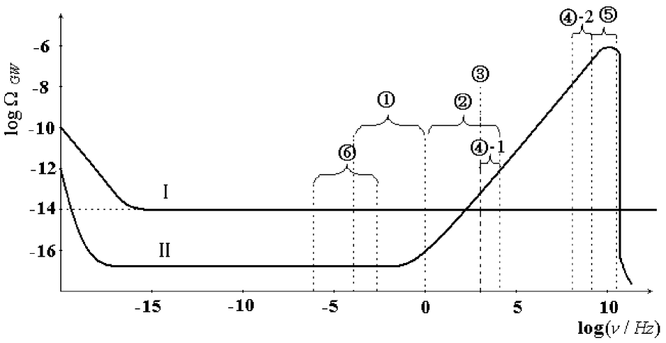
Figure 1: Curves I and II represent the relic graviton logarithmic energy spectra (in critical units) expected by the usual ordinary inflationary models and by the quintessential inflationary models, respectively. The curves quote from Ref.[1]. Here we illustrate roughly the distribution for some detecting-frequency bands. The region (1) expresses the detecting frequency band of LISA ($\sim{10^{-4}}-1Hz$); the region (2) is one of LIGO ($\sim{1}-10^{4}Hz$); the region (3) is one of the resonant-mass detectors ($\sim{10^{3}}Hz$); the region (4)-1 is one of the difference-frequency resonant response of the microwave cavities ($\sim 10^{3}-10^{4}Hz$), the region (4)-2 ($\sim 10^{8}-10^{9}Hz$) is one of the fundamental resonant response of the microwave cavities; the region (5) is one of the Gaussian beams ($\sim{10^{9}}-10^{11}Hz$) and region (6) is one of Mini-ASTROD ($\sim 10^{-6}-10^{-3}Hz$). It can be seen that the region (4)-2 coincides partly with the maximal signal and peak of the relic graviton energy spectra expected by the quintessential inflationary models, the detecting frequency band (5) of the Gaussian beam tuned in on GHz frequency region can be almost completely localized in this peak value region. For the relevant background in figure 1, we presented a brief introduction in Appendixes (Appendix A: The cavity electromagnetic response to the GW’s. Appendix B: The dimensionless amplitude $h$ and the power spectrum $S_{h}$ of the relic GW’s. Appendix C: ASTROD. Appendix D: Noise problems).

Giovannini[1] analyzed the relic GW’s in the quintessential inflationary models within a framework of quantum theory. In this framework the Fourier expansion of the field operators of the relic GW’s can be written as

$$\hat{\mu}_{\oplus}(\vec{x},\eta)=\frac{1}{(2\pi)^{3/2}}\int d^{3}k_{g}[\hat{\mu}_{\oplus}(k_{g},\eta)\;e^{i\vec{k_{g}}.\vec{x}}+\hat{\mu}_{\oplus}^{\ast}(k_{g},\eta)\;e^{-i\vec{k_{g}}.\vec{x}}],$$

$$\hat{\mu}_{\otimes}(\vec{x},\eta)=\frac{1}{(2\pi)^{3/2}}\int d^{3}k_{g}[\hat{\mu}_{\otimes}(k_{g},\eta)\;e^{i\vec{k_{g}}.\vec{x}}+\hat{\mu}_{\otimes}^{\ast}(k_{g},\eta)\;e^{-i\vec{k_{g}}.\vec{x}}],$$ (12)

where

$$\hat{\mu}_{\oplus}(k_{g},\eta)=\psi_{\oplus}(k_{g},\eta)\hat{a}_{\oplus}(k_{g}),$$

$$\hat{\mu}_{\otimes}(k_{g},\eta)=\psi_{\otimes}(k_{g},\eta)\hat{a}_{\otimes}(k_{g}),$$ (13)

$\oplus$ and $\otimes$ denote + and $\times$ polarization of the GW’s, respectively, $\eta$ is the conformal time, $\hat{a}_{\oplus}^{*}$ , $\hat{a}_{\otimes}^{*}$ and $\hat{a}_{\oplus}$, $\hat{a}_{\otimes}$ represent the creation and annihilation operators of the above two physical polarization states. From the viewpoint of observation, the classical picture of Eq.(12) corresponds to the amplitudes of the relic GW’s with the states of the two polarization, namely,

$$h_{\oplus}(\vec{x},\eta)=\frac{1}{(2\pi)^{3/2}}\int d^{3}k_{g}\;h_{\oplus}(k_{g},\eta)\;e^{i\vec{k_{g}}.\vec{x}},$$

$$h_{\otimes}(\vec{x},\eta)=\frac{1}{(2\pi)^{3/2}}\int d^{3}k_{g}\;h_{\otimes}(k_{g},\eta)\;e^{i\vec{k_{g}}.\vec{x}},$$ (14)

where the integration spreads over the whole frequency band of the relic GW’s. However, if we hope to realize the resonant response of a monochromatic Gaussian beam to the relic GW’s, it is necessary to let the frequency of the Gaussian beam equals a certain frequency in the peak value region of the relic GW’s (i.e., $\omega_{e}=\omega_{g}$). Fortunately, most of strong microwave beams (including the Gaussian beam) generated by present technology are monochromatic or quasi-monochromatic, thus resonateable relic GW to the Gaussian beam will be only one monochromatic component of satisfying condition $\omega_{g}=\omega_{e}$ in the relic GW frequency band. In this case the corresponding treatment can be greatly simplified without excluding the essential physical features. Of course, for the resonant response to the relic GW’s on the earth, we should use interval of laboratory time (i.e., $c\;dt=a(\eta)\;d\eta$) and laboratory frequency[27]. Consequently, a monochromatic circular polarized plan relic GW propagating along the $z$-axis can be written as

$$h_{\oplus}=h_{xx}=-h_{yy}=A_{\oplus}\;\exp({ik_{\alpha}x^{\alpha}})=A_{\oplus}\exp{[i(k_{g}z-\omega_{g}t)]},$$

$$h_{\otimes}=h_{xy}=h_{yx}=iA_{\otimes}\;\exp({ik_{\alpha}x^{\alpha}})=iA_{\otimes}\exp{[i(k_{g}z-\omega_{g}t)]}.$$ (15)

This is just usual form of the GW in the TT gauge. Eq.(15) can be viewed as the classical approximation of the Eqs.(12) and (13) under the monochromatic wave condition.

Since the relic GW’s in the peak value region of the quintessential inflationary models have very high frequency (the GHz frequency band), future measurements through the microwave cavities or the strong Gaussian beams may be useful. Especially, for the high-frequency relic GW’s of $10^{9}$ Hz $\leq\nu_{g}\leq 10^{11}$ Hz (these are just best peak frequency band expected by the quintessential inflationary models), using the EM response of the Gaussian beam would be more suitable (see Fig.1).

III.2 The electromagnetic system in the high-frequency relic gravitational wave field

From Eq.(15), the nonvanishing components of metric tensor in Cartesian coordinates are given by

$$g_{00}=-1,\qquad g_{11}=g_{xx}=1+h_{xx}=1+h_{\oplus},\qquad g_{22}=g_{yy}=1+h_{yy}=1-h_{\oplus},$$

$$g_{12}=g_{21}=g_{xy}=g_{yx}=h_{xy}=h_{\otimes},\qquad g_{33}=g_{zz}=1,$$

$$g^{00}=-1,\qquad g^{11}=g^{xx}=1-h^{xx}=1-h_{\oplus},\qquad g^{22}=g^{yy}=1-h^{yy}=1+h_{\oplus},$$

$$g^{12}=g^{21}=g^{xy}=g^{yx}=-h^{xy}=-h_{\otimes},\qquad g^{33}=g^{zz}=1.$$ (16)

With the help of Eqs.(3)–(8) and considering perturbation produced be the weak GW field expressed as Eqs.(15) and (16), the components of the EM field tensor in the Cartesian coordinates can be written as

$$F_{01}=\tilde{F}_{01}^{(0)}+\tilde{F}_{01}^{(1)}=\frac{1}{c}(\tilde{E}_{x}^{(0)}+\tilde{E}_{x}^{(1)})=\frac{1}{c}(\psi+\tilde{E}_{x}^{(1)}),$$

$$F_{02}=\tilde{F}_{02}^{(1)}=\frac{1}{c}\tilde{E}_{y}^{(1)},\qquad F_{03}=\tilde{F}_{03}^{(1)}=\frac{1}{c}\tilde{E}_{z}^{(1)},$$

$$F_{12}=\tilde{F}_{12}^{(0)}+\tilde{F}_{12}^{(1)}=-(\tilde{B}_{z}^{(0)}+\tilde{B}_{z}^{(1)})=-(\frac{i}{\omega}\frac{\partial{\psi}}{\partial{y}}+\tilde{B}_{z}^{(1)}),$$

$$F_{13}=\hat{F}_{13}^{(0)}+\tilde{F}_{13}^{(0)}+\tilde{F}_{13}^{(1)}=\hat{B}_{y}^{(0)}+\tilde{B}_{y}^{(0)}+\tilde{B}_{y}^{(1)}=\hat{B}_{y}^{(0)}-\frac{i}{\omega}\frac{\partial{\psi}}{\partial{z}}+\tilde{B}_{y}^{(1)},$$

$$F_{23}=\tilde{F}_{23}^{(1)}=\tilde{B}_{x}^{(1)},$$ (17)

where $\hat{F}_{\mu\nu}^{(0)}$ and $\tilde{F}_{\mu\nu}^{(0)}$ represent the background static magnetic field $\hat{B}_{y}^{(0)}$ and the background EM wave field (the Gaussian beam), respectively, $\tilde{F}_{\mu\nu}^{(1)}$ is the first-order perturbation to the background EM fields in the presence of the GW. For the nonvanishing $F_{\mu\nu}^{(0)}$ and $F_{\mu\nu}^{(1)}$, we have $\left|\tilde{F}_{\mu\nu}^{(1)}\right|\ll\left|F_{\mu\nu}^{(0)}\right|$.

The EM response to the GW can be described by Maxwell equations in curved space-time, i.e.,

$$\frac{1}{\sqrt{-g}}\frac{\partial}{\partial{x^{\nu}}}(\sqrt{-g}\;g^{\mu\alpha}g^{\nu\beta}F_{\alpha\beta})=\mu_{0}J^{\mu},$$ (18)

$$F_{[\mu\nu,\alpha]}=0,$$ (19)

where $J^{\mu}$ indicates the four-dimensional electric current density. For the EM response in the vacuum, because it has neither the real four-dimensional electric current nor the equivalent electric current caused by the energy dissipation, such as Ohmic losses in the cavity electrodynamical response or the dielectric losses[10], so that $J^{\mu}=0\;$ in Eq.(18).

Unlike the interaction of a plane EM wave with a plane GW (according to the Einstein-Maxwell equations under the condition of the weak gravitational field, if both the plane GW and plane EM wave have the same propagating direction, then the perturbation of GW to the EM wave vanishes[17])., the electric and magnetic fields of the Gaussian beam are nonsymmetric (see Eqs.(1) and (5)-(8)). In this case, using Eqs.(5)-(8) and (18)-(19), it can be shown that even for the plane GW propagating along the positive $z$-direction, it can produce nonvanishing perturbative effect to the Gaussian beam. In order to find the concrete form of the perturbation produced by the direct interaction of the GW with the Gaussian beam, it is necessary to solve Eqs.(18) and (19) by substituting Eqs.(1), (5)-(8), (15), (16) and (17) into them, which is often quite difficult. However, as shown in Refs.[8, 17, 28, 29], the orders of amplitudes of the first-order perturbative electric and magnetic fields produced by the direct interaction of the GW with the EM wave (e. g., plane wave or the Gaussian beam) are approximately $h\tilde{B}^{(0)}c\;$ and $h\tilde{B}^{(0)}$, respectively, while that generated by the direct interaction of the GW with the static magnetic field are approximately $h\hat{B}^{(0)}c\;$ and $h\hat{B}^{(0)}$ respectively. Thus corresponding amplitude ratio is about $h\tilde{B}^{(0)}/h\hat{B}^{(0)}$. In our case, we have chosen $\tilde{B}^{(0)}\sim{10^{-3}}T$, $\hat{B}^{(0)}\sim{10}T$, i.e., their ratio is only $10^{-4}$ roughly. Therefore, the former can be neglected. In other words, the contribution of the Gaussian beam is mainly expressed as the coherent synchroresonance (i.e., $\omega_{e}=\omega_{g}$) of it with the first-order perturbation $\tilde{F}_{\mu\nu}^{(1)}$ generated by the direct interaction of the GW with the static field $\hat{B}_{y}^{(0)}$. In this case, solving the process of Eqs.(18) and (19) can be greatly simplified, i.e., the static magnetic field $\hat{B}^{(0)}=\hat{B}^{(0)}_{y}$ can be seen as the unique background EM field in Eqs.(18) and (19). Under these circumstances, in the first we can solve Eqs.(18) and (19) in the region II ($-l/2\leq z\leq l/2,\;\hat{B}^{(0)}=\hat{B}_{y}^{(0)}$) to find the first-order perturbation solutions; and second, using the boundary conditions one can obtain the first-order perturbation solutions in the region I ($z\leq-l/2,\;\hat{B}^{(0)}=0$) and the region III ($z\geq l/2,\;\hat{B}^{(0)}=0$).

Introducing Eqs.(15)-(17) into Eqs.(18)-(19), neglecting high-order infinite small quantities and perturbative effect produced by the direct interaction of the GW with Gaussian beam, Eqs.(18) and (19) are reduced to

$$\frac{1}{c^{2}}\tilde{E}^{(1)}_{x,t}+\tilde{B}^{(1)}_{y,z}=\hat{B}_{y}^{(0)}h_{xx,z},$$

$$\tilde{E}^{(1)}_{x,z}+\tilde{B}^{(1)}_{y,t}=0,$$ (20)

$$\frac{1}{c^{2}}\tilde{E}^{(1)}_{y,t}+\tilde{B}^{(1)}_{x,z}=\hat{B}_{y}^{(0)}h_{xy,z},$$

$$\tilde{E}^{(1)}_{y,z}-\tilde{B}^{(1)}_{x,t}=0,$$ (21)

and

$$\tilde{E}^{(1)}_{z,t}=\tilde{E}^{(1)}_{z,z}=0,\qquad\tilde{B}^{(1)}_{z,t}=\tilde{B}^{(1)}_{z,z}=0,$$ (22)

where the commas denote partial derivatives. Using Eq.(15), Eqs.(20)-(22) can also be expressed as following inhomogeneous hyperbolic-type equations, respectively:

$$\square\tilde{E}_{x}^{(1)}=\tilde{E}_{x,zz}^{(1)}-\frac{1}{c^{2}}\tilde{E}_{x,tt}^{(1)}=-A_{\oplus}\hat{B}_{y}^{(0)}k_{g}^{2}\,c\,\exp{[i(k_{g}z-\omega_{g}t)]},$$

$$\square\tilde{B}_{y}^{(1)}=\tilde{B}_{y,zz}^{(1)}-\frac{1}{c^{2}}\tilde{B}_{y,tt}^{(1)}=-A_{\oplus}\hat{B}_{y}^{(0)}k_{g}^{2}\,\exp{[i(k_{g}z-\omega_{g}t)]},$$ (23)

$$\square\tilde{E}_{y}^{(1)}=\tilde{E}_{y,zz}^{(1)}-\frac{1}{c^{2}}\tilde{E}_{y,tt}^{(1)}=-iA_{\otimes}\hat{B}_{y}^{(0)}k_{g}^{2}\,c\,\exp{[i(k_{g}z-\omega_{g}t)]},$$

$$\square\tilde{B}_{x}^{(1)}=\tilde{B}_{x,zz}^{(1)}-\frac{1}{c^{2}}\tilde{B}_{x,tt}^{(1)}=iA_{\otimes}\hat{B}_{y}^{(0)}k_{g}^{2}\,\exp{[i(k_{g}z-\omega_{g}t)]},$$ (24)

$$\square\tilde{E}_{z}^{(1)}=\square\tilde{B}_{z}^{(1)}=0,$$ (25)

where $\square$ indicates the d’Alembertian. Obviously, every solution of Eq.(20) must satisfy Eq.(23), and every solution of Eq.(21) must satisfy Eq.(24), and it is easily seen from Eqs.(22) and (25), that a physically reasonable solution of them would be only

$$\tilde{E}_{z}^{(1)}=\tilde{B}_{z}^{(1)}=0.$$ (26)

The general solutions of Eqs.(20)-(24) in the region II ($-l/2\leq z\leq l/2$) are given by

$$\tilde{E}_{x}^{(1)}=\frac{i}{2}A_{\oplus}\hat{B}_{y}^{(0)}k_{g}\,c\,(z+l/2)\exp{[i(k_{g}z-\omega_{g}t)]}+b_{1}\exp{[i(k_{g}z-\omega_{g}t)]}+c_{1}\exp{[i(k_{g}z+\omega_{g}t)]},$$

$$\tilde{B}_{y}^{(1)}=\frac{i}{2}A_{\oplus}\hat{B}_{y}^{(0)}k_{g}(z+l/2)\exp{[i(k_{g}z-\omega_{g}t)]}+b_{2}\exp{[i(k_{g}z-\omega_{g}t)]}+c_{2}\exp{[i(k_{g}z+\omega_{g}t)]},$$ (27)

$$\tilde{E}_{y}^{(1)}=-\frac{1}{2}A_{\otimes}\hat{B}_{y}^{(0)}k_{g}\,c\,(z+l/2)\exp{[i(k_{g}z-\omega_{g}t)]}+ib_{3}\exp{[i(k_{g}z-\omega_{g}t)]}+ic_{3}\exp{[i(k_{g}z+\omega_{g}t)]},$$

$$\tilde{B}_{x}^{(1)}=\frac{1}{2}A_{\otimes}\hat{B}_{y}^{(0)}k_{g}(z+l/2)\exp{[i(k_{g}z-\omega_{g}t)]}+ib_{4}\exp{[i(k_{g}z-\omega_{g}t)]}+ic_{4}\exp{[i(k_{g}z+\omega_{g}t)]}.$$ (28)

The solutions (26)-(28) show that perturbative EM waves produced by the plane GW satisfing TT gauge, must be the transverse waves, and the background static magnetic field is perpendicular to the propagating direction of the GW. The constants in Eqs.(27) and (28) satisfy

$$b_{1}-cb_{2}=-\frac{1}{2}A_{\oplus}\hat{B}_{y}^{(0)}c,\qquad c_{1}+cc_{2}=0,$$

$$b_{3}+cb_{4}=-\frac{1}{2}A_{\otimes}\hat{B}_{y}^{(0)}c,\qquad c_{3}-cc_{4}=0,$$ (29)

their concrete forms will be defined by the physical requirements and boundary conditions.

The solutions (26)-(28) have the similar features as that found by a number of authors [28, 29] previously, but as we shall show that unlike the previous works, our EM system will be a possible scheme to display the first-order EM perturbations produced by the high-frequency relic GW’s (GHz region) inside of the typical laboratory size (not necessarily interferometers or EM cavities with giant dimensions), a particularly interesting feature of the first-order perturbation will be the perturbative effect in the some special directions and in the some special regions.

It should be pointed out that in curved space-time, only local measurements made by an observer travelling in his world-line have definite observable meaning. These observable quantities are just the projections of the physical quantities as the tensor on tetrads of the observer’s world-line. The tetrads consist of three space-like mutually orthogonal vectors and a time-like vector directed along the four-velocity of the observer, the latter is perpendicular to the preceding ones. We indicate these with $\tau^{\mu}_{(\alpha)}$, where the index in brackets numbers the vectors and the other refers to the components of the tetrads in the chosen coordinates. Consequently, the quantities $F_{(\alpha\beta)}$ measured by the observer are the tetrad components of the EM field tensor, that is

$$F_{(\alpha\beta)}=F_{\mu\nu}\tau^{\mu}_{(\alpha)}\tau^{\nu}_{(\beta)}.$$ (30)

Obviously, for our EM system, the observer should be laid at rest state to the static magnetic field, i.e., only the zeroth-component of his four-velocity nonvanish. Thus, the tetrad $\tau^{\mu}_{(0)}$ has the form

$$\tau^{\mu}_{(0)}=(\tau^{0}_{(0)},\;0,\;0,\;0).$$ (31)

Using Eq.(16) and the orthonormality of the tetrads   $g_{\mu\nu}\tau^{\mu}_{(\alpha)}\tau^{\nu}_{(\beta)}=\eta_{\alpha\beta}$,  neglecting high-order infinite small quantities, it is always possible to get

$$\tau^{\mu}_{(0)} = (1,\;0,\;0,\;0),$$

$$\tau^{\mu}_{(1)} = (0,\;1-\frac{1}{2}h_{\oplus},\;0,\;0),$$

$$\tau^{\mu}_{(2)} = (0,\;-h_{\otimes},\;1+\frac{1}{2}h_{\oplus},\;0),$$

$$\tau^{\mu}_{(3)} = (0,\;0,\;0,\;1).$$ (32)

Eq.(32) indicates that the zeroth and third components of the tetrads coincide completely with the time- and $z$-axes in the chosen coordinates, respectively. Furthermore, $\tau^{\mu}_{(1)}$ has only the projection on the $x$-axis, thus $\tau^{\mu}_{(1)}$ points actually at the $x$-axis. This means that the azimuth $\phi$ in the tetrads and that in the chosen coordinates are the same. While the deviation of $\tau^{\mu}_{(2)}$ from the $y$-axis is only an order of $h_{\otimes}$.

With the help of Eqs.(3),(4),(27),(28) and (32), neglecting high-order infinite small quantities, we obtain

$$E_{(x)}=cF_{(01)}=cF_{\mu\nu}\tau^{\mu}_{(0)}\tau^{\nu}_{(1)}=\tilde{E}_{x}^{(0)}+\tilde{E}_{x}^{(1)}-\frac{1}{2}h_{xx}\tilde{E}_{x}^{(0)}=\psi+\tilde{E}_{x}^{(1)}-\frac{1}{2}h_{\oplus}\psi\;,$$

$$E_{(y)}=cF_{(02)}=cF_{\mu\nu}\tau^{\mu}_{(0)}\tau^{\nu}_{(2)}=\tilde{E}_{y}^{(1)}-h_{\otimes}\psi\;,$$

$$E_{(z)}=cF_{(03)}=cF_{\mu\nu}\tau^{\mu}_{(0)}\tau^{\nu}_{(3)}=0\;,$$

$$B_{(x)}=F_{(32)}=F_{\mu\nu}\tau^{\mu}_{(3)}\tau^{\nu}_{(2)}=\tilde{B}_{x}^{(1)}+h_{xy}(\hat{B}_{y}^{(0)}+\tilde{B}_{y}^{(0)})=\tilde{B}_{x}^{(1)}+h_{\otimes}(\hat{B}_{y}^{(0)}-\frac{i}{\omega_{e}}\frac{\partial\psi}{\partial z})\;,$$

$$B_{(y)}=F_{(13)}=F_{\mu\nu}\tau^{\mu}_{(1)}\tau^{\nu}_{(3)}=\hat{B}_{y}^{(0)}+\tilde{B}_{y}^{(0)}+\tilde{B}_{y}^{(1)}=\hat{B}_{y}^{(0)}-\frac{i}{\omega_{e}}\frac{\partial\psi}{\partial z}+\tilde{B}_{y}^{(1)}\;,$$

$$B_{(z)}=F_{(21)}=F_{\mu\nu}\tau^{\mu}_{(2)}\tau^{\nu}_{(1)}=\tilde{B}_{z}^{(0)}=\frac{i}{\omega_{e}}\frac{\partial\psi}{\partial y}\;.$$ (33)

As we have pointed out above, here $|h\tilde{F}_{\mu\nu}^{(0)}|\sim A\tilde{B}^{(0)}$ , $|\tilde{F}_{\mu\nu}^{(1)}|\sim A\hat{B}^{(0)}_{y}$ ,  and in our case, $\hat{B}^{(0)}\sim 10T\,,\,\tilde{B}^{(0)}\sim 10^{-3}T\,,\,$ thus we have $|h\tilde{F}_{\mu\nu}^{(0)}|/|\tilde{F}_{\mu\nu}^{(1)}|\;\approx\tilde{B}^{(0)}/\hat{B}_{y}^{(0)}\approx 10^{-4}$ ,  so that  $h\tilde{F}_{\mu\nu}^{(0)}$  terms in Eq.(33) can be neglected again. In this case Eq.(33) can be further reduced to (in the region II: $-l/2\leq z\leq l/2$)

$$E_{(x)} = \psi+\tilde{E}_{x}^{(1)}$$

$$= \psi+\frac{i}{2}A_{\oplus}\hat{B}_{y}^{(0)}k_{g}\,c\,(z+l/2)\exp{[i(k_{g}z-\omega_{g}t)]}+b_{1}\exp{[i(k_{g}z-\omega_{g}t)]}+c_{1}\exp{[i(k_{g}z+\omega_{g}t)]},$$

$$B_{(y)} = \hat{B}_{y}^{(0)}-\frac{i}{\omega_{e}}\frac{\partial\psi}{\partial z}+\tilde{B}_{y}^{(1)}$$ (34)

$$= \hat{B}_{y}^{(0)}-\frac{i}{\omega_{e}}\frac{\partial\psi}{\partial z}+\frac{i}{2}A_{\oplus}\hat{B}_{y}^{(0)}k_{g}(z+l/2)\exp{[i(k_{g}z-\omega_{g}t)]}+b_{2}\exp{[i(k_{g}z-\omega_{g}t)]}$$

$$+ c_{2}\exp{[i(k_{g}z+\omega_{g}t)]},$$

$$E_{(y)} = \tilde{E}_{y}^{(1)}$$

$$= -\frac{1}{2}A_{\otimes}\hat{B}_{y}^{(0)}k_{g}\,c\,(z+l/2)\exp{[i(k_{g}z-\omega_{g}t)]}+ib_{3}\exp{[i(k_{g}z-\omega_{g}t)]}+ic_{3}\exp{[i(k_{g}z+\omega_{g}t)]},$$

$$B_{(x)} = \tilde{B}_{x}^{(1)}+h_{\otimes}\hat{B}_{y}^{(0)}$$ (35)

$$= \frac{1}{2}A_{\otimes}\hat{B}_{y}^{(0)}k_{g}(z+l/2)\exp{[i(k_{g}z-\omega_{g}t)]}+ib_{4}\exp{[i(k_{g}z-\omega_{g}t)]}+ic_{4}\exp{[i(k_{g}z+\omega_{g}t)]}$$

$$+iA_{\otimes}\hat{B}_{y}^{(0)}\exp{[i(k_{g}z-\omega_{g}t)]},$$

and

$$E_{(z)}=0,$$

$$B_{(z)}=\tilde{B}_{z}^{(0)}=\frac{i}{\omega_{e}}\frac{\partial\psi}{\partial y}\;\;_{.}$$ (36)

III.3 The particular solutions satisfying boundary conditions

In fact, the perturbative parts in Eqs.(34)-(36) are the general solutions of Eqs.(20)-(25) in the region II ($-l/2\leq z\leq l/2$). We shall define the constants in Eqs.(34) and (35) to give the corresponding particular solutions satisfying the boundary conditions.

Clearly, the perturbative EM fields in the regions I, II and III must satisfy the boundary conditions (the continuity conditions):

$$(\tilde{F}^{\;(1)}_{(\mu\nu)I})_{z=-l/2}\;\;=\;\;(\tilde{F}^{\;\,(1)}_{(\mu\nu)II})_{z=-l/2}\;,\qquad(\tilde{F}^{\;\,(1)}_{(\mu\nu)II})_{z=l/2}\;\;=\;\;(\tilde{F}^{\;\;(1)}_{(\mu\nu)III})_{z=l/2}\;{}_{.}$$ (37)

If one chooses the real part of the pure perturbative fields in Eqs.(34) and (35), then we have

$$\tilde{E}^{(1)}_{(x)} = -\frac{1}{2}A_{\oplus}\hat{B}_{y}^{(0)}k_{g}\,c\,(z+l/2)\sin{(k_{g}z-\omega_{g}t)}+b_{1}\cos{(k_{g}z-\omega_{g}t)}+c_{1}\cos{(k_{g}z+\omega_{g}t)},$$

$$\tilde{B}^{(1)}_{(y)} = -\frac{1}{2}A_{\oplus}\hat{B}_{y}^{(0)}k_{g}(z+l/2)\sin{(k_{g}z-\omega_{g}t)}+b_{2}\cos{(k_{g}z-\omega_{g}t)}+c_{2}\cos{(k_{g}z+\omega_{g}t)},$$ (38)

$$\tilde{E}^{(1)}_{(y)} = -\frac{1}{2}A_{\otimes}\hat{B}_{y}^{(0)}k_{g}\,c\,(z+l/2)\cos{(k_{g}z-\omega_{g}t)}-b_{3}\sin{(k_{g}z-\omega_{g}t)}-c_{3}\sin{(k_{g}z+\omega_{g}t)},$$

$$\tilde{B}^{(1)}_{(x)} = \frac{1}{2}A_{\otimes}\hat{B}_{y}^{(0)}k_{g}(z+l/2)\cos{(k_{g}z-\omega_{g}t)}-b_{4}\sin{(k_{g}z-\omega_{g}t)}-c_{4}\sin{(k_{g}z+\omega_{g}t)}$$ (39)

$$-A_{\otimes}\hat{B}_{y}^{(0)}\sin{(k_{g}z-\omega_{g}t)}.$$

A physically reasonable requirement is that there is no the perturbative EM wave propagating along the negative $z$-direction in the region III($z\geq l/2$). Here we shall consider one more simple case, i.e., the perturbative EM wave in the negative $z$-direction is also absent in the region I($z\leq-l/2$). In order to satisfy the boundary conditions, Eq.(37), and the above requirement, from Eqs.(29) and (37)-(39), one finds

$$b_{1}=-\frac{1}{4}A_{\oplus}\hat{B}_{y}^{(0)}c,\qquad b_{2}=\frac{1}{4}A_{\oplus}\hat{B}_{y}^{(0)},\qquad b_{3}=\frac{1}{4}A_{\otimes}\hat{B}_{y}^{(0)}c,\qquad b_{4}=-\frac{3}{4}A_{\otimes}\hat{B}_{y}^{(0)},$$

$$c_{1}=\frac{1}{4}A_{\oplus}\hat{B}_{y}^{(0)}c,\qquad c_{2}=-\frac{1}{4}A_{\oplus}\hat{B}_{y}^{(0)},\qquad c_{3}=\frac{1}{4}A_{\otimes}\hat{B}_{y}^{(0)}c,\qquad c_{4}=\frac{1}{4}A_{\otimes}\hat{B}_{y}^{(0)},$$

(40)

and

$$l=n\lambda_{g}\;\;\;\;\;(n\;\;\rm{is\;\;integer}).$$ (41)

In this case we have the perturbative EM fields in the above three regions as follows:

(a)  Region I ($z\leq-l/2$, $\hat{B}^{(0)}=0$)

$$\tilde{E}_{(x)}^{(1)}=c\tilde{F}_{(01)}^{(1)}=\tilde{E}_{(y)}^{(1)}=c\tilde{F}_{(02)}^{(1)}=0,$$

$$\tilde{B}_{(x)}^{(1)}=\tilde{F}_{(32)}^{(1)}=\tilde{B}_{(y)}^{(1)}=\tilde{F}_{(13)}^{(1)}=0.$$ (42)

(b)  Region II ($-l/2\leq z\leq l/2$, $\hat{B}^{(0)}=\hat{B}_{y}^{(0)}$)

$$\tilde{E}_{(x)}^{(1)} = -\frac{1}{2}A_{\oplus}\hat{B}_{y}^{(0)}k_{g}\,c\,(z+l/2)\sin{(k_{g}z-\omega_{g}t)}-\frac{1}{2}A_{\oplus}\hat{B}_{y}^{(0)}\,c\,\sin{(k_{g}z)}\sin{(\omega_{g}t)},$$

$$\tilde{B}_{(y)}^{(1)} = -\frac{1}{2}A_{\oplus}\hat{B}_{y}^{(0)}k_{g}(z+l/2)\sin{(k_{g}z-\omega_{g}t)}+\frac{1}{2}A_{\oplus}\hat{B}_{y}^{(0)}\sin{(k_{g}z)}\sin{(\omega_{g}t)},$$ (43)

$$\tilde{E}_{(y)}^{(1)} = -\frac{1}{2}A_{\otimes}\hat{B}_{y}^{(0)}k_{g}\,c\,(z+l/2)\cos{(k_{g}z-\omega_{g}t)}-\frac{1}{2}A_{\otimes}\hat{B}_{y}^{(0)}\,c\,\sin{(k_{g}z)}\cos{(\omega_{g}t)},$$

$$\tilde{B}_{(x)}^{(1)} = \frac{1}{2}A_{\otimes}\hat{B}_{y}^{(0)}k_{g}(z+l/2)\cos{(k_{g}z-\omega_{g}t)}-\frac{1}{2}A_{\otimes}\hat{B}_{y}^{(0)}\sin{(k_{g}z)}\cos{(\omega_{g}t)},$$ (44)

(c)  Region III ($l/2\leq z\leq l_{0},\hat{B}^{(0)}=0$)

$$\tilde{E}_{(x)}^{(1)} = -\frac{1}{2}A_{\oplus}\hat{B}_{y}^{(0)}k_{g}\,c\,l\,\sin{(k_{g}z-\omega_{g}t)},$$

$$\tilde{B}_{(y)}^{(1)} = -\frac{1}{2}A_{\oplus}\hat{B}_{y}^{(0)}k_{g}\,l\,\sin{(k_{g}z-\omega_{g}t)},$$ (45)

$$\tilde{E}_{(y)}^{(1)} = -\frac{1}{2}A_{\otimes}\hat{B}_{y}^{(0)}k_{g}\,c\,l\,\cos{(k_{g}z-\omega_{g}t)},$$

$$\tilde{B}_{(x)}^{(1)} = \frac{1}{2}A_{\otimes}\hat{B}_{y}^{(0)}k_{g}\,l\,\cos{(k_{g}z-\omega_{g}t)},$$ (46)

where $l_{0}$ is the size of the effective region in which the second-order perturbative EM power fluxes, such as $\frac{1}{\mu_{0}}(\tilde{E}_{(x)}^{(1)}\tilde{B}_{(y)}^{(1)})$,  $\frac{1}{\mu_{0}}(\tilde{E}_{(y)}^{(1)}\tilde{B}_{(x)}^{(1)})$,  keep a plane wave form. Notice that the power fluxes in the region II contain the parts with space accumulation effect, i.e., they depend upon the square of the interaction dimension. This is because the GW’s and EM waves have same velocity, so that the two waves can generate an optimum coherent effect in the propagating direction. It is easily to show that if we choose the imaginary part of the pure perturbative fields in Eqs.(34) and (35), we can obtain the similar results, but Eq.(41) will be replaced by

$$l=(2n+1)\frac{\lambda_{g}}{2}\;\;\;(n\;\;\rm{is\;\;integer}).$$ (47)

Logi and Mickelson [29] used Feynmann perturbation techniques to analyze the perturbative EM waves (photon fluxes) produced by a weak GW (gravitons) passing through a static magnetic (or an electrostatic) field, and found that perturbative EM waves (photon fluxes) propagate only in the same and in the opposite propagating directions of the GW(gravitons), the latter is weaker than the former, or the latter is absent. Obviously, our results and calculation by Logi et.al are self-consistent. However, due to the weakness of the interaction of the GW’s(gravitons) with the EM fields(photons), we shall focus our attention on the first-order perturbative power fluxes produced by the coherent synchroresonance of the above perturbative EM fields with the background Gaussian beam, not only the second-order perturbative EM power fluxes themselves, such as $\frac{1}{\mu_{0}}(\tilde{E}_{(x)}^{(1)}\tilde{B}_{(y)}^{(1)})$  and $\frac{1}{\mu_{0}}(\tilde{E}_{(y)}^{(1)}\tilde{B}_{(x)}^{(1)})$.

III.4 The first-order perturbative electromagnetic power fluxes

The generic expression of the energy-momentum tensor of the EM fields in the GW fields is given by

$$T^{\mu\nu}=\frac{1}{{\mu_{0}}}\left({-F_{\;\;{\rm}\alpha}^{\mu}F^{\nu\alpha}+\frac{1}{4}g^{\mu\nu}F_{\alpha\beta}F^{\alpha\beta}}\right).$$

Due to $F_{\mu\nu}=F_{\mu\nu}^{(0)}+\tilde{F}_{\mu\nu}^{(1)}$ and $\left|{\tilde{F}_{\mu\nu}^{(1)}}\right|<<\left|{F_{\mu\nu}^{(0)}}\right|$ for the nonvanishing $F_{\mu\nu}^{(0)}$ and $\tilde{F}_{\mu\nu}^{(1)}$, $T^{\mu\nu}$ can be disintegrated into

$$T^{\mu\nu}=\mathop{T^{\mu\nu}}\limits^{(0)}+\mathop{T^{\mu\nu}}\limits^{(1)}+\mathop{T^{\mu\nu}}\limits^{(2)},$$ (49)

where $\mathop{T^{\mu\nu}}\limits^{(0)}$ is the energy-momentum tensor of the background EM fields, and $\mathop{T^{\mu\nu}}\limits^{(1)}$ and $\mathop{T^{\mu\nu}}\limits^{(2)}$ represent first- and second-order perturbations to $\mathop{T^{\mu\nu}}\limits^{(0)}$ in the presence of the GW, respectively.

Using Eq.(16), $\mathop{T^{{}^{\mu\nu}}}\limits^{(0)}$, $\mathop{T^{{}^{\mu\nu}}}\limits^{(1)}$ and $\mathop{T^{{}^{\mu\nu}}}\limits^{(2)}$ can be written as

$$\mathop{T^{{}^{\mu\nu}}}\limits^{(0)}=\frac{1}{{\mu_{0}}}\left({-F_{{\;\;\rm}\alpha}^{\mu{\rm}(0)}F^{\nu\alpha(0)}+\frac{1}{4}\eta^{\mu\nu}F_{\alpha\beta}^{(0)}F^{\alpha\beta(0)}}\right),$$ (50)

$$\mathop{T^{{}^{\mu\nu}}}\limits^{(1)}=\frac{1}{{\mu_{0}}}\left[{-\left({F_{{\;\;\rm}\alpha}^{\mu{\rm}(0)}\tilde{F}^{\nu\alpha(1)}+\tilde{F}_{{\;\;\rm}\alpha}^{\mu{\rm}(1)}F^{\nu\alpha(0)}}\right)+\frac{1}{4}\eta^{\mu\nu}\left({\tilde{F}_{\alpha\beta}^{(1)}F^{\alpha\beta(0)}+F_{\alpha\beta}^{(0)}\tilde{F}^{\alpha\beta(1)}}\right)-\frac{1}{4}h^{\mu\nu}F_{\alpha\beta}^{(0)}F^{\alpha\beta(0)}}\right],$$

$$\mathop{T^{{}^{\mu\nu}}}\limits^{(2)}=\frac{1}{{\mu_{0}}}\left[{-\tilde{F}_{\;\;{\rm}\alpha}^{\mu{\rm}(1)}\tilde{F}^{\nu\alpha(1)}+\frac{1}{4}\eta^{\mu\nu}\tilde{F}_{\alpha\beta}^{(1)}\tilde{F}^{\alpha\beta(1)}-\frac{1}{4}h^{\mu\nu}\left({F_{\alpha\beta}^{(0)}\tilde{F}^{\alpha\beta(1)}+\tilde{F}_{\alpha\beta}^{(1)}F^{\alpha\beta(0)}}\right)}\right].$$ (52)

For the nonvanishing $\mathop{T^{{}^{\mu\nu}}}\limits^{(0)}$, $\mathop{T^{{}^{\mu\nu}}}\limits^{(1)}$ and $\mathop{T^{{}^{\mu\nu}}}\limits^{(2)}$, we have

$$|\mathop{T^{\mu\nu}}\limits^{(0)}|\gg|\mathop{T^{\mu\nu}}\limits^{(1)}|\gg|\mathop{T^{\mu\nu}}\limits^{(2)}|.$$ (53)

Therefore, for the effect of the GW, we are interested in $\mathop{T^{{}^{\mu\nu}}}\limits^{(1)}$ but not in $\mathop{T^{{}^{\mu\nu}}}\limits^{(0)}$ and $\mathop{T^{{}^{\mu\nu}}}\limits^{(2)}$. Nevertheless, it can be shown from Eqs.(1), (3), (5)-(8),(15), (42)-(46) and (52), that the average value of $\mathop{T^{{}^{00}}}\limits^{(2)}$ with respect to time is always positive. Thus it expresses essentially the net increasing quantity of the energy density of the EM fields. Especially, under the resonant conditions, it should correspond to the resonant graviton-photon conversion at a quantum level [29, 30, 31]. But because of $|\mathop{T^{\mu\nu}}\limits^{(2)}|<<|\mathop{T^{\mu\nu}}\limits^{(1)}|$ for the nonvanishing $\mathop{T^{\mu\nu}}\limits^{(1)}$ and $\mathop{T^{\mu\nu}}\limits^{(2)}$ , the second-order perturbations are often far below the requirements of the observable effect. In this case it has only theoretical interest. However, for some astrophysical situations, it is possible to cause observable effects, because where very large EM fields and very strong GW’s often occur simultaneously and these fields extend over a very large area [32, 33].

By using Eqs.(1), (3), (5)-(8), (15), (42)-(46) and (51). we obtain

$$\mathop{S^{r}}\limits^{(1)}=c\mathop{T^{01}}\limits^{(1)}=\frac{1}{{\mu_{0}}}\left({\tilde{E}_{(\phi)}^{(1)}\tilde{B}_{(z)}^{(0)}}\right)=-\frac{1}{{\mu_{0}}}\left({\tilde{E}_{(x)}^{(1)}\tilde{B}_{(z)}^{(0)}}\right)\sin\phi+\frac{1}{{\mu_{0}}}\left({\tilde{E}_{(y)}^{(1)}\tilde{B}_{(z)}^{(0)}}\right)\cos\phi,$$ (54)

$$\mathop{S^{\phi}}\limits^{(1)}=c\mathop{T^{02}}\limits^{(1)}=-\frac{1}{{\mu_{0}}}\left({\tilde{E}_{(r)}^{(1)}\tilde{B}_{(z)}^{(0)}}\right)=-\frac{1}{{\mu_{0}}}\left({\tilde{E}_{(x)}^{(1)}\tilde{B}_{(z)}^{(0)}}\right)\cos\phi-\frac{1}{{\mu_{0}}}\left({\tilde{E}_{(y)}^{(1)}\tilde{B}_{(z)}^{(0)}}\right)\sin\phi,$$ (55)

$$\mathop{S^{z}}\limits^{(1)}=c\mathop{T^{03}}\limits^{(1)}=\frac{1}{{\mu_{0}}}\left({\tilde{E}_{(x)}^{(0)}\tilde{B}_{(y)}^{(1)}}\right)+\frac{1}{{\mu_{0}}}\left({\tilde{E}_{(x)}^{(1)}\tilde{B}_{(y)}^{(0)}}\right).$$ (56)

where $\mathop{S^{r}}\limits^{(1)}$ ,$\mathop{S^{\phi}}\limits^{(1)}$ and $\mathop{S^{z}}\limits^{(1)}$ represent the first-order radial, tangential and axial perturbative power flux densities, respectively. As we have shown above, that for the high-frequency perturbative power fluxes, only nonvanishing average values of them with respect to time have observable effect. It is easily seen from Eqs.(1), (5)-(8) and (42)-(46), that average values of the perturbative power flux densities. Eqs.(54)-(56),vanish in whole frequency rang of $\omega_{e}\neq\omega_{g}$. In other words, only under the condition of $\omega_{e}=\omega_{g}$ (synchroresonance), $\mathop{S^{r}}\limits^{(1)}$ , $\mathop{S^{\phi}}\limits^{(1)}$ and $\mathop{S^{z}}\limits^{(1)}$ have nonvanishing average values with respect to time.

In the following we study only the tangential average power flux density $<{\mathop{S^{\phi}}\limits^{(1)}}>_{\omega_{e}=\omega_{g}}$. Introducing Eqs.(1), (8), (42)-(46) into (55), and setting $\delta=\pi/2$ in Eq.(1) (it is always possible), we have

$$<{\mathop{S^{\phi}}\limits^{(1)}}>_{\omega_{e}=\omega_{g}}=<{\mathop{S_{\oplus}^{\phi}}\limits^{(1)}}>_{\omega_{e}=\omega_{g}}+<{\mathop{S_{\otimes}^{\phi}}\limits^{(1)}}>_{\omega_{e}=\omega_{g}},$$ (57)

where

$$<{\mathop{S_{\oplus}^{\phi}}\limits^{(1)}}>_{\omega_{e}=\omega_{g}}=-\frac{1}{{\mu_{0}}}<{\tilde{E}_{(x)}^{(1)}\tilde{B}_{(z)}^{(0)}}>\cos\phi,$$

$$<{\mathop{S_{\otimes}^{\phi}}\limits^{(1)}}>_{\omega_{e}=\omega_{g}}=-\frac{1}{{\mu_{0}}}<{\tilde{E}_{(y)}^{(1)}\tilde{B}_{(z)}^{(0)}}>\sin\phi.$$ (58)

$<{\mathop{S_{\oplus}^{\phi}}\limits^{(1)}}>_{\omega_{e}=\omega_{g}}$ and $<{\mathop{S_{\otimes}^{\phi}}\limits^{(1)}}>_{\omega_{e}=\omega_{g}}$ represent the average values of the first-order tangential perturbative power flux densities generated by the states of $+$ polarization and $\times$ polarization of the GW, Eq.(15), respectively. Using Eqs.(1), (8), (42)-(46), (57), (58) and the boundary conditions [see, Eqs. (37) and (41)], one finds

(a)  Region I  ($z\leq-l/2$),

$$<{\mathop{S_{\oplus}^{\phi}}\limits^{(1)}}>_{\omega_{e}=\omega_{g}}=<{\mathop{S_{\otimes}^{\phi}}\limits^{(1)}}>_{\omega_{e}=\omega_{g}}=0.$$ (59)

(b)  Region II  ($-l/2\leq z\leq l/2$),

$$<{\mathop{S_{\oplus}^{\phi}}\limits^{(1)}}>_{\omega_{e}=\omega_{g}}=\left\{{\frac{{A_{\oplus}\hat{B}_{y}^{(0)}\psi_{0}k_{g}r\left({z+{l\mathord{\left/{\vphantom{l2}}\right.\kern-1.2pt}2}}\right)}}{{8\mu_{0}\left[{1+\left({{z\mathord{\left/{\vphantom{zf}}\right.\kern-1.2pt}f}}\right)^{2}}\right]^{1/2}\left({z+{{f^{2}}\mathord{\left/{\vphantom{{f^{2}}z}}\right.\kern-1.2pt}z}}\right)}}}\right.\cos\left({\tan^{-1}\frac{z}{f}-\frac{{k_{g}r^{2}}}{{2R}}}\right)$$

$$+\frac{{A_{\oplus}\hat{B}_{y}^{(0)}\psi_{0}r\left({z+{l\mathord{\left/{\vphantom{l2}}\right.\kern-1.2pt}2}}\right)}}{{4\mu_{0}W_{0}^{2}\left[{1+\left({{z\mathord{\left/{\vphantom{zf}}\right.\kern-1.2pt}f}}\right)^{2}}\right]^{3/2}}}\sin\left({\tan^{-1}\frac{z}{f}-\frac{{k_{g}r^{2}}}{{2R}}}\right)$$

$$-\frac{{A_{\oplus}\hat{B}_{y}^{(0)}\psi_{0}r}}{{8\mu_{0}\left[{1+\left({{z\mathord{\left/{\vphantom{zf}}\right.\kern-1.2pt}f}}\right)^{2}}\right]^{1/2}\left({z+{{f^{2}}\mathord{\left/{\vphantom{{f^{2}}z}}\right.\kern-1.2pt}z}}\right)}}\sin\left({k_{g}z}\right)\cos\left({\tan^{-1}\frac{z}{f}-\frac{{k_{g}r^{2}}}{{2R}}-k_{g}z}\right)$$

$$-\frac{{A_{\oplus}\hat{B}_{y}^{(0)}\psi_{0}r}}{{4\mu_{0}k_{g}W_{0}^{2}\left[{1+\left({{z\mathord{\left/{\vphantom{zf}}\right.\kern-1.2pt}f}}\right)^{2}}\right]^{3/2}}}\sin\left({k_{g}z}\right)\sin\left.{\left({\tan^{-1}\frac{z}{f}-\frac{{k_{g}r^{2}}}{{2R}}-k_{g}z}\right)}\right\}\exp(-\frac{r^{2}}{W^{2}})\sin\left({2\phi}\right),$$ (60)

$$<{\mathop{S_{\otimes}^{\phi}}\limits^{(1)}}>_{\omega_{e}=\omega_{g}}=\left\{{\frac{{A_{\otimes}\hat{B}_{y}^{(0)}\psi_{0}k_{g}r\left({z+{l\mathord{\left/{\vphantom{l2}}\right.\kern-1.2pt}2}}\right)}}{{4\mu_{0}\left[{1+\left({{z\mathord{\left/{\vphantom{zf}}\right.\kern-1.2pt}f}}\right)^{2}}\right]^{1/2}\left({z+{{f^{2}}\mathord{\left/{\vphantom{{f^{2}}z}}\right.\kern-1.2pt}z}}\right)}}}\right.\sin\left({\frac{{k_{g}r^{2}}}{{2R}}-\tan^{-1}\frac{z}{f}}\right)$$

$$+\frac{{A_{\otimes}\hat{B}_{y}^{(0)}\psi_{0}r\left({z+{l\mathord{\left/{\vphantom{l2}}\right.\kern-1.2pt}2}}\right)}}{{2\mu_{0}W_{0}^{2}\left[{1+\left({{z\mathord{\left/{\vphantom{zf}}\right.\kern-1.2pt}f}}\right)^{2}}\right]^{3/2}}}\cos\left({\frac{{k_{g}r^{2}}}{{2R}}-\tan^{-1}\frac{z}{f}}\right)$$

$$+\frac{{A_{\otimes}\hat{B}_{y}^{(0)}\psi_{0}r}}{{4\mu_{0}\left[{1+\left({{z\mathord{\left/{\vphantom{zf}}\right.\kern-1.2pt}f}}\right)^{2}}\right]^{1/2}\left({z+{{f^{2}}\mathord{\left/{\vphantom{{f^{2}}z}}\right.\kern-1.2pt}z}}\right)}}\sin\left({k_{g}z}\right)\sin\left({k_{g}z-\tan^{-1}\frac{z}{f}+\frac{{k_{g}r^{2}}}{{2R}}}\right)$$

$$+\frac{{A_{\otimes}\hat{B}_{y}^{(0)}\psi_{0}r}}{{2\mu_{0}k_{g}W_{0}^{2}\left[{1+\left({{z\mathord{\left/{\vphantom{zf}}\right.\kern-1.2pt}f}}\right)^{2}}\right]^{3/2}}}\sin\left({k_{g}z}\right)\cos\left.{\left({k_{g}z-\tan^{-1}\frac{z}{f}+\frac{{k_{g}r^{2}}}{{2R}}}\right)}\right\}\exp(-\frac{r^{2}}{W^{2}})\sin^{2}\phi.$$ (61)

(c)  Region III  ($l/2\leq z\leq l_{0}$),

$$<{\mathop{S_{\oplus}^{\phi}}\limits^{(1)}}>_{\omega_{e}=\omega_{g}}=\left\{{\frac{{A_{\oplus}\hat{B}_{y}^{(0)}\psi_{0}k_{g}lr}}{{8\mu_{0}\left[{1+\left({{z\mathord{\left/{\vphantom{zf}}\right.\kern-1.2pt}f}}\right)^{2}}\right]^{1/2}\left({z+{{f^{2}}\mathord{\left/{\vphantom{{f^{2}}z}}\right.\kern-1.2pt}z}}\right)}}}\right.\cos\left({\tan^{-1}\frac{z}{f}-\frac{{k_{g}r^{2}}}{{2R}}}\right)$$

$$+\frac{{A_{\oplus}\hat{B}_{y}^{(0)}\psi_{0}lr}}{{4\mu_{0}W_{0}^{2}\left[{1+\left({{z\mathord{\left/{\vphantom{zf}}\right.\kern-1.2pt}f}}\right)^{2}}\right]^{3/2}}}\sin\left.{\left({\tan^{-1}\frac{z}{f}-\frac{{k_{g}r^{2}}}{{2R}}}\right)}\right\}\exp(-\frac{r^{2}}{W^{2}})\sin\left({2\phi}\right),$$ (62)

$$<{\mathop{S_{\otimes}^{\phi}}\limits^{(1)}}>_{\omega_{e}=\omega_{g}}=\left\{{\frac{{A_{\otimes}\hat{B}_{y}^{(0)}\psi_{0}k_{g}lr}}{{4\mu_{0}\left[{1+\left({{z\mathord{\left/{\vphantom{zf}}\right.\kern-1.2pt}f}}\right)^{2}}\right]^{1/2}\left({z+{{f^{2}}\mathord{\left/{\vphantom{{f^{2}}z}}\right.\kern-1.2pt}z}}\right)}}}\right.\sin\left({\frac{{k_{g}r^{2}}}{{2R}}-\tan^{-1}\frac{z}{f}}\right)$$

$$+\frac{{A_{\otimes}\hat{B}_{y}^{(0)}\psi_{0}lr}}{{2\mu_{0}W_{0}^{2}\left[{1+\left({{z\mathord{\left/{\vphantom{zf}}\right.\kern-1.2pt}f}}\right)^{2}}\right]^{3/2}}}\cos\left.{\left({\frac{{k_{g}r^{2}}}{{2R}}-\tan^{-1}\frac{z}{f}}\right)}\right\}\exp(-\frac{r^{2}}{W^{2}})\sin^{2}\phi.$$ (63)

It is easily shown that the nonvanishing first-order perturbative power flux densities are much greater than corresponding second-order perturbative power flux densities. The quantum picture of this process can be described as the interaction of the photons with the gravitons in a background of virtual photons (or virtual gravitons) as a catalyst [29, 34], which can greatly increase the interacting cross section between the photons and gravitons. In other words the interaction may effectively change the physical behavior (e.g., propagating direction, distribution, polarization and phase) of the photons in the local regions, even if the net increasing quantities of the photon number (the EM energy) of the entire EM system approach zero, such properties may be very useful to display very weak signals of the GW’s.

Eqs. (60)-(63) show that because there are nonvanishing ${\mathop{S_{\oplus}^{\phi}}\limits^{(1)}}$ (which depends on the $+$ polarization state of the GW) and ${\mathop{S_{\otimes}^{\phi}}\limits^{(1)}}$ (which depends on the $\times$ polarization state of the GW), the first-order tangential perturbative power fluxes are expressed as the “left circular wave” and “right circular wave” in the cylindrical polar coordinates, which around the symmetrical axis of the Gaussian beam, but $<{\mathop{S_{\oplus}^{\phi}}\limits^{(1)}}>_{\omega_{e}=\omega_{g}}$ and $<{\mathop{S_{\otimes}^{\phi}}\limits^{(1)}}>_{\omega_{e}=\omega_{g}}$ have a different physical behavior. By comparing Eqs.(60)-(63) with Eqs.(9)-(11), we can see that: (a)$<{\mathop{S_{\oplus}^{\phi}}\limits^{(1)}}>_{\omega_{e}=\omega_{g}}$ and $<{\mathop{S^{\phi}}\limits^{(0)}}>$ have the same angular distribution factor $sin(2\phi)$ , thus $<{\mathop{S_{\oplus}^{\phi}}\limits^{(1)}}>_{\omega_{e}=\omega_{g}}$ will be swamped by the background power flux $<{\mathop{S^{\phi}}\limits^{(0)}}>$. Namely, in this case $<{\mathop{S_{\oplus}^{\phi}}\limits^{(1)}}>_{\omega_{e}=\omega_{g}}$ has no observable effect. (b) The angular distribution factor of $<{\mathop{S_{\otimes}^{\phi}}\limits^{(1)}}>_{\omega_{e}=\omega_{g}}$ is a $sin^{2}\phi$ , it is different from that of $<{\mathop{S^{\phi}}\limits^{(0)}}>$. Therefore,$<{\mathop{S_{\otimes}^{\phi}}\limits^{(1)}}>_{\omega_{e}=\omega_{g}}$,in principle, has an observable effect. In particular, at the surfaces $\phi=\pi/2,3\pi/2$, $<{\mathop{S^{\phi}}\limits^{(0)}}>\equiv 0$, while $|{<{\mathop{S_{\otimes}^{\phi}}\limits^{(1)}}>_{\omega_{e}=\omega_{g}}}|=|{<{\mathop{S_{\otimes}^{\phi}}\limits^{(1)}}>_{\omega_{e}=\omega_{g}}}|_{\max}$ , this is satisfactory (although $<{\mathop{S^{r}}\limits^{(0)}}>$ and ${<{\mathop{S_{\otimes}^{\phi}}\limits^{(1)}}>_{\omega_{e}=\omega_{g}}}$ have the same angular distribution factor $sin^{2}\phi$, the propagating direction of $<{\mathop{S^{r}}\limits^{(0)}}>$ is perpendicular to that of $<\mathop{S_{\otimes}^{\phi}}\limits^{(1)}>_{\omega_{e}=\omega_{g}}$ , thus $<\mathop{S^{r}}\limits^{(0)}>$ (including $<{\mathop{S^{z}}\limits^{(0)}}>$ ) has no any essentially contribution in the pure tangential direction).

Figure 2 gives the distribution of $<{\mathop{S_{\oplus}^{\phi}}\limits^{(1)}}>_{\omega_{e}=\omega_{g}}$ at the plane $z=l/2=\frac{n}{2}\lambda_{g}$ (n is a integer) in the cylindrical polar coordinates, while figure 3 gives the distribution of $<{\mathop{S_{\otimes}^{\phi}}\limits^{(1)}}>_{\omega_{e}=\omega_{g}}$ at the plane $z=0$ in the cylindrical polar coordinates.

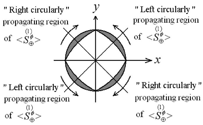
Figure 2: Distribution of $<{\mathop{S_{\oplus}^{\phi}}\limits^{(1)}}>_{\omega_{e}=\omega_{g}}$ at the plane $z=l/2=\frac{n}{2}\lambda_{g}$ (n is integer) in the cylindrical polar coordinates. It has maximum at $\phi=\pi/4,3\pi/4,5\pi/4,$ and $7\pi/4$, while it vanishes at $\phi=0,\pi/2,\pi$ and $3\pi/2$, here $l=0.1m$,$\lambda_{g}=0.01m$ and $r=0.05m$, and the GW propagates along the $z$-axis.

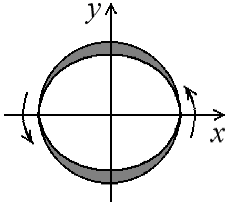
Figure 3: Distribution of $<{\mathop{S_{\otimes}^{\phi}}\limits^{(1)}}>_{\omega_{e}=\omega_{g}}$ at the plane $z=0$ in the cylindrical polar coordinates. It has maximum at $\phi=\pi/2$ and $3\pi/2$,while it vanishes at $\phi=0,\pi$, Unlike figure 2, $<{\mathop{S_{\otimes}^{\phi}}\limits^{(1)}}>_{\omega_{e}=\omega_{g}}$ at the $z=0$ is completely “left-hand circular”, here $r=0.05m$, $\lambda_{g}=0.01m$, and the GW propagates along the $z$-axis.

From Eqs.(10),(11),(60) and (61), we can also see that $<{\mathop{S^{r}}\limits^{(0)}}>=<{\mathop{S^{\phi}}\limits^{(0)}}>=<{\mathop{S_{\oplus}^{\phi}}\limits^{(1)}}>_{\omega_{e}=\omega_{g}}\equiv 0$ at the plane $z=0$, while where

$$<{\mathop{S_{\otimes}^{\phi}}\limits^{(1)}}>_{\omega_{e}=\omega_{g}}=\frac{{A_{\otimes}\hat{B}_{y}^{(0)}\psi_{0}lr}}{{4\mu_{0}W_{0}^{2}}}\exp\left({-\frac{{r^{2}}}{{W_{0}^{2}}}}\right)\sin^{2}\phi.$$ (64)

In Table I we list the distribution of $<\mathop{S^{\phi}}\limits^{(0)}>$ , $<\mathop{S_{\oplus}^{\phi}}\limits^{(1)}>_{\omega_{e}=\omega_{g}}$ and $<\mathop{S_{\otimes}^{\phi}}\limits^{(1)}>_{\omega_{e}=\omega_{g}}$ in some typical regions.

Table 1: The distribution of $<{\mathop{S^{\phi}}\limits^{(0)}}>$,$<{\mathop{S_{\oplus}^{\phi}}\limits^{(1)}}>_{\omega_{e}=\omega_{g}}$and $<{\mathop{S_{\otimes}^{\phi}}\limits^{(1)}}>_{\omega_{e}=\omega_{g}}$ in some typical regions

	Angular distribution	The plane	The planes	The planes	The planes
	factor	$z=0$	$\phi=\pi/4,5\pi/4$	$\phi=3\pi/4,7\pi/4$	$\phi=\pi/2,3\pi/2$
$<{\mathop{S^{\phi}}\limits^{(0)}}>$	$sin(2\phi)$	0	$|{<{\mathop{S^{\phi}}\limits^{(0)}}>}|=|{<{\mathop{S^{\phi}}\limits^{(0)}}>}|_{\max}$,	$|{<{\mathop{S^{\phi}}\limits^{(0)}}>}|=|{<{\mathop{S^{\phi}}\limits^{(0)}}>}|_{\max},$	0
			“Left circularly”	“Right circularly”
			propagation.	propagation.
$<{\mathop{S_{\oplus}^{\phi}}\limits^{(1)}}>_{\omega_{e}=\omega_{g}}$	$sin(2\phi)$	0	$|{<{\mathop{S_{\oplus}^{\phi}}\limits^{(1)}}>_{\omega_{e}=\omega_{g}}}|=$	$|{<{\mathop{S_{\oplus}^{\phi}}\limits^{(1)}}>_{\omega_{e}=\omega_{g}}}|=$	0
			$|{<{\mathop{S_{\oplus}^{\phi}}\limits^{(1)}}>_{\omega_{e}=\omega_{g}}}|_{\max},$	$|{<{\mathop{S_{\oplus}^{\phi}}\limits^{(1)}}>_{\omega_{e}=\omega_{g}}}|_{\max}$ ,
			“Left circularly”	“Right circularly”
			propagation.	propagation.
${<{\mathop{S_{\otimes}^{\phi}}\limits^{(1)}}>_{\omega_{e}=\omega_{g}}}$	$sin^{2}\phi$	$|{<{\mathop{S_{\otimes}^{\phi}}\limits^{(1)}}>_{\omega_{e}=\omega_{g}}}|=$	There are	There are	$|{<{\mathop{S_{\otimes}^{\phi}}\limits^{(1)}}>_{\omega_{e}=\omega_{g}}}|=$
		$|{<{\mathop{S_{\otimes}^{\phi}}\limits^{(1)}}>_{\omega_{e}=\omega_{g}}}|_{\max}$	nonvanishing values,	nonvanishing values,	$|{<{\mathop{S_{\otimes}^{\phi}}\limits^{(1)}}>_{\omega_{e}=\omega_{g}}}|_{\max}$,
		at $\phi=\pi/2,3\pi/2$	“Left circularly”	“Left circularly”	“Left circularly”
			propagation.	propagation.	propagation.

Table I, Eqs.(60)-(63) and Figures 2, 3 show that the plane $z=0$ and the planes $\phi=\pi/2,\;\;3\pi/2$ are the three most interesting regions. For the former, $<\mathop{S^{\phi}}\limits^{(0)}>=<\mathop{S^{r}}\limits^{(0)}>=<\mathop{S_{\oplus}^{\phi}}\limits^{(1)}>_{\omega_{e}=\omega_{g}}\equiv 0$, but nonvanishing $<\mathop{S_{\otimes}^{\phi}}\limits^{(1)}>_{\omega_{e}=\omega_{g}}$ exists; for the latter, $<\mathop{S^{\phi}}\limits^{(0)}>=<\mathop{S_{\oplus}^{\phi}}\limits^{(0)}>_{\omega_{e}=\omega_{g}}\equiv 0$, but there is non-zero $<\mathop{S_{\otimes}^{\phi}}\limits^{(1)}>_{\omega_{e}=\omega_{g}}$. This means that any nonvanishing tangential EM power flux in such regions will express the pure electromagnetic-gravitational perturbation.

III.5 Numerical estimations

If we describe the perturbation in the quantum language (photon flux), the corresponding perturbative photon flux $n_{\phi}$ caused by $<\mathop{S_{\otimes}^{\phi}}\limits^{(1)}>_{\omega_{e}=\omega_{g}}$ at the plane $\phi=\pi/2$ (we note that $<\mathop{S_{\otimes}^{\phi}}\limits^{(1)}>_{\omega_{e}=\omega_{g}}$ is the unique nonvanishing power flux density passing through the plane) can be given by

$$n_{\phi}=\frac{{<\mathop{u_{\otimes}^{\phi}}\limits^{(1)}>_{\omega_{e}=\omega_{g},\;\phi={\pi\mathord{\left/{\vphantom{\pi 2}}\right.\kern-1.2pt}2}}}}{{\hbar\omega_{e}}}=\frac{1}{{\hbar\omega_{e}}}\int_{0}^{W_{0}}{\int_{-l/2}^{l_{0}}{<\mathop{S_{\otimes}^{\phi}}\limits^{(1)}>_{\omega_{e}=\omega_{g},\;\phi=\pi/2}}}dzdr,$$ (65)

where $<\mathop{u_{\otimes}^{\phi}}\limits^{(1)}>_{\omega_{e}=\omega_{g},\;\phi={\pi\mathord{\left/{\vphantom{\pi 2}}\right.\kern-1.2pt}2}}=\int_{0}^{W_{0}}{\int_{-{l\mathord{\left/{\vphantom{l2}}\right.\kern-1.2pt}2}}^{l_{0}}{<\mathop{S_{\otimes}^{\phi}}\limits^{(1)}>_{\omega_{e}=\omega_{g},\;\phi={\pi\mathord{\left/{\vphantom{\pi 2}}\right.\kern-1.2pt}2}}}}dzdr$ is the total perturbative power flux passing through the plane $\phi=\pi/2$, $\hbar$ is the Planck constant.

In order to give reasonable estimation,we choose the achievable values of the EM parameters in the present experiments: (1)$\psi_{0}=3\times 10^{5}V.m^{-1}$ (i. e., $\psi_{0}/c=10^{-3}T$), the amplitude of the Gaussian beam. If the spot radius $W_{0}$ of the Gaussian beam is limited in $0.05m$, the corresponding power can be estimated as $P=\int_{0}^{W_{0}}{<\mathop{S^{z}}\limits^{(0)}>_{z=0}2\pi rdr\approx 10^{5}W}$ (see Eq. (9)), this power is well within the current technology condition [21, 35]. For the Gaussian beam with $\nu_{e}=3\times 10^{10}Hz$, this is equivalent to a photon flux $n^{(0)}$ of $3\times 10^{28}s^{-1}$ roughly. (2)$\hat{B}_{y}^{(0)}=30T$, the strength of the background static magnetic field, this is achievable strength of a stationary magnetic field under the present experimental condition [36]. (3) $A_{\otimes}=10^{-30}$, $\omega_{g}/2\pi=\nu_{g}=3\times 10^{10}Hz$, these are the typical orders expected by the quintessential inflationary models [1]. Substituting Eqs.(61),(63) and the above parameters into Eq.(65), and setting $W_{0}=0.05m,l=0.1m,l_{0}=0.3m$,we obtain $n_{\phi}\approx 1.57\times 10^{3}s^{-1}$ (see Table II). Up to now, this is largest perturbative photon flux in a series of results [7, 8, 9]. Recently, we analyzed and estimated them under the typical laboratory parameter conditions. If the integration region of the radial coordinate $r$ in Eq.(65) is moved to $W_{0}\leq r\leq r_{0}$ (here $W_{0}=0.05m$, $r_{0}=0.1m$), in the same way, the corresponding perturbative photon flux $n^{\prime}_{\phi}$ can be estimated as $n^{\prime}_{\phi}=\frac{1}{{\hbar\omega_{e}}}\int_{W_{0}}^{r_{0}}{\int_{-l/2}^{l_{0}}{<\mathop{S^{\phi}_{\otimes}}\limits^{(1)}>_{\omega_{e}=\omega_{g},\phi=\pi/2}dzdr=0.96\times 10^{3}}}s^{-1}\approx 10^{3}s^{-1}$. Although then $n^{\prime}_{\phi}<n_{\phi}$, it retains basically order of $10^{3}s^{-1}$, and because the “receiving” plane of the tangential perturbative photon flux is already moved to the region outside the spot radius $W_{0}$ of the Gaussian beam, it has more realistic meaning to distinguish and display the perturbative photon flux.

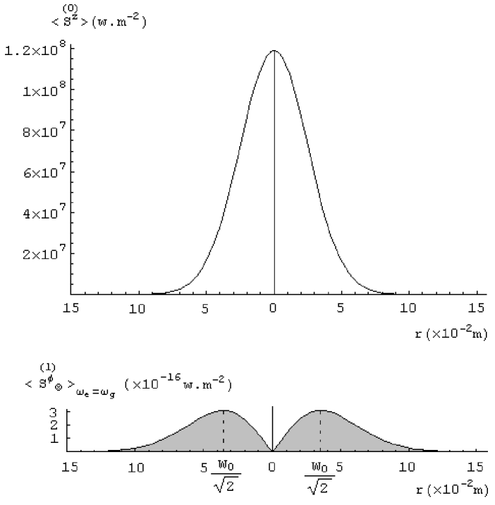
Figure 4: Rating curve between $<\mathop{S_{\otimes}^{\phi}}\limits^{(1)}>_{\omega_{e}=\omega_{g}}$ and $<\mathop{S^{z}}\limits^{(0)}>$ at the plane $z=0$, hers $r$ is the radial coordinate, and $\phi=\pi/2$ or $3\pi/2$ in Eq.(64). It shows that $|<\mathop{S_{\otimes}^{\phi}}\limits^{(1)}>_{\omega_{e}=\omega_{g}}|=|<\mathop{S_{\otimes}^{\phi}}\limits^{(1)}>_{\omega_{e}=\omega_{g}}|_{\max}$ at $r=W_{0}/\sqrt{2}$. The background axial power flux density $<\mathop{S^{z}}\limits^{(0)}>$ is typical Gaussian distribution, and $|<\mathop{S^{z}}\limits^{(0)}>|>>|<\mathop{S_{\otimes}^{\phi}}\limits^{(1)}>_{\omega_{e}=\omega_{g}}|_{\max}$. However, because the propagating direction of $<\mathop{S^{z}}\limits^{(0)}>$ is perpendicular to that of $<\mathop{S_{\otimes}^{\phi}}\limits^{(1)}>_{\omega_{e}=\omega_{g}}$, $<\mathop{S^{z}}\limits^{(0)}>$ has no any contribution in the pure tangential direction. The shaded part expresses $<\mathop{S_{\otimes}^{\phi}}\limits^{(1)}>_{\omega_{e}=\omega_{g}}$. Here $\nu_{e}=\nu_{g}=\omega_{g}/2\pi=3\times 10^{10}Hz$, $A_{\otimes}=10^{-30}$, $\hat{B}_{y}^{(0)}=30T$, $\psi_{0}=3\times 10^{5}V.m^{-1}$, $l=0.1m$, $W_{0}=0.05m$.

Figure 4 gives the rating curve between $<{\mathop{S_{\otimes}^{\phi}}\limits^{(1)}}>_{\omega_{e}=\omega_{g}}$ and $<{\mathop{S^{z}}\limits^{(0)}}>$ at the plane $z=0$, here $r$ is the radial coordinate.

Figure 5 gives the rating curve between $n_{\phi}$ and the axis coordinate $z$, and relative parameters are chosen as $\nu_{e}=\nu_{g}=\omega_{g}/2\pi=3\times 10^{10}Hz$, $A_{\otimes}=10^{-30}$, $\hat{B}_{y}^{(0)}=30T$, $\psi_{0}=3\times 10^{5}V.m^{-1}$, $l=0.1m$, $l_{0}=0.3m$ and $W_{0}=0.05m$. Figure 5 shows that $n_{\phi}$ has a good space accumulation effect as $z$ increases. In fact, in addition to the third- and fourth-terms in Eq.(61), the rest in the expression of $<\mathop{S_{\otimes}^{\phi}}\limits^{(1)}>_{\omega_{e}=\omega_{g}}$, Eq.(61) and Eq.(63), is all slow enough variational function at the $z$ direction. This means that the value of $<\mathop{S_{\otimes}^{\phi}}\limits^{(1)}>_{\omega_{e}=\omega_{g}}$ is slow variational and keeps its sign invariant in the whole region of the coherent resonance (here it is about the region of $80\lambda_{g}$, namely $0.8m$), that they make $<\mathop{S_{\otimes}^{\phi}}\limits^{(1)}>_{\omega_{e}=\omega_{g}}$ being all “left circularly” propagated from $-l/2$ to $l_{o}$.

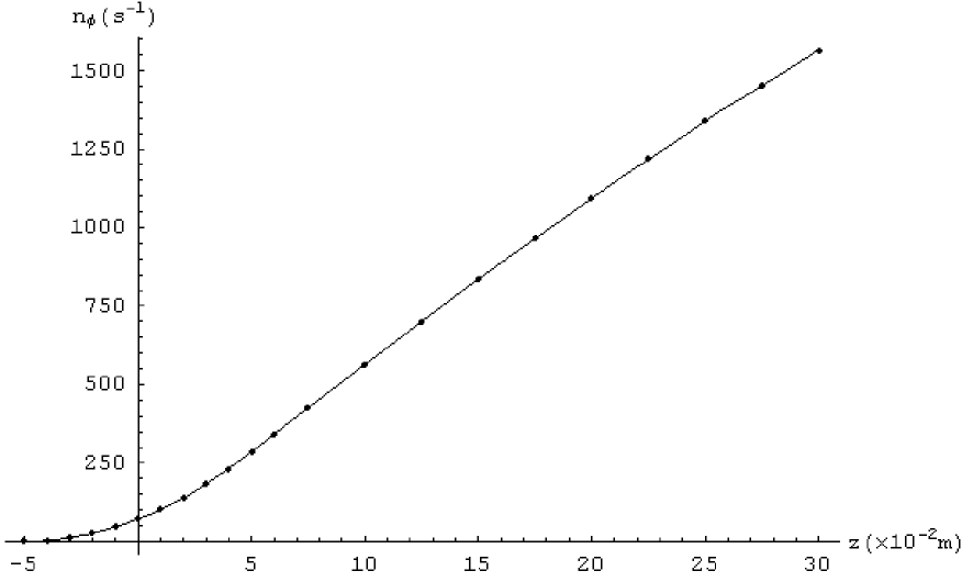
Figure 5: Rating curve between $n_{\phi}$ and the axial coordinate $z$, here $\nu_{e}=\nu_{g}=\omega_{g}/2\pi=3\times 10^{10}Hz$, $A_{\otimes}=10^{-30}$, $\hat{B}_{y}^{(0)}=30T$, $\psi_{0}=3\times 10^{5}V.m^{-1}$, and $W_{0}=0.05m$. It shows that the pure tangential perturbative photon flux passing through the plane $\phi=\pi/2$ with $10^{-2}m^{2}$, would be expected to be $1.57\times 10^{3}s^{-1}$.

Table II gives the tangential perturbative photon fluxes and corresponding relevant parameters in the three cases. In the first case $W_{01}=0.05m$, in the second case $W_{02}=0.02m$, in the third case $W_{03}=0.1m$, but the background Gaussian beam keep the same power in such three cases, i. e., $P\approx 10^{5}W$. Due to $W_{03}>W_{01}>W_{02}$, so that $\psi_{03}<\psi_{01}<\psi_{02}$. Table II shows that the tangential perturbation in the Gaussian beam with larger $W_{0}$ (i. e., smaller $\theta$) has a better physical effect than that in the Gaussian beam with smaller $W_{0}$ (i. e., larger $\theta$), here $\theta$ is the spreading angle of the beam, $\theta=tan^{-1}({\frac{{\lambda_{e}}}{{\pi W_{0}}}})\approx{\frac{{\lambda_{e}}}{{\pi W_{0}}}}$ .

Table 2: The tangential perturbative photon fluxes and corresponding relevant parameters

	$A$	$\nu_{g}(Hz)$	$W_{0}(m)$	$\theta$	$<{\mathop{u_{\otimes}^{\phi}}\limits^{(1)}}>_{\omega_{e}=\omega_{g}}$ (W)	$n_{\phi}(s^{-1})$
(1)	$10^{-30}$	$3\times 10^{10}$	$\;\;\;\;\;0.05\;\;\;\;\;\;$	$6.36\times 10^{-2}$	$\;\;\;\;3.11\times 10^{-20}\;\;\;\;$	$\;\;\;1.57\times 10^{3}\;\;\;$
(2)	$10^{-30}$	$3\times 10^{10}$	$0.02$	$15.78\times 10^{-2}$	$1.31\times 10^{-20}$	$6.61\times 10^{2}$
(3)	$\;\;\;\;10^{-30}\;\;\;\;\;$	$3\times 10^{10}$	$0.10$	$3.18\times 10^{-2}$	$3.14\times 10^{-20}$	$1.58\times 10^{3}$

We emphasize that here $n_{\phi}\propto\psi_{0}\propto\sqrt{P}$ (see Eqs.(61), (63), and (65), $P$ is the power of the Gaussian beam), and at the same time, $n_{\phi}\propto\hat{B}_{y}^{(0)}$. Therefore, if $P$ is reduced to $10^{3}W$, then $n_{\phi}\approx 1.57\times 10^{2}s^{-1}$; and even if $P$ is reduced to $10W$ (this is already a very relaxed requirement), we have still $n_{\phi}\approx 1.57\times 10s^{-1}$. Thus, if possible, increasing $\hat{B}_{y}^{(0)}$ (in this way the number of the background real photons does not change) has better physical effect than increasing $P$. According to the above discussion, we give some values for the power $P$ of the background Gaussian beam and corresponding parameters $n_{\phi}$ and $n^{\prime}_{\phi}$ (see Table III).

Table 3: The power of the background Gaussian beam and corresponding $n_{\phi}$ and $n^{\prime}_{\phi}$.

$\;\;\;\;\;\;\;\;\;\;P(W)\;\;\;\;\;\;\;\;\;\;$	$\;\;\;\;\;\;\;\;\;\;n_{\phi}(s^{-1})\;\;\;\;\;\;\;\;\;\;$	$\;\;\;\;\;\;\;\;\;\;n^{\prime}_{\phi}(s^{-1})\;\;\;\;\;\;\;\;\;\;$
$10^{5}$	$\sim 1.57\times 10^{3}$	$\sim 10^{3}$
$10^{3}$	$\sim 1.57\times 10^{2}$	$\sim 10^{2}$
$10$	$\sim 1.57\times 10$	$\sim 10$

In particular, since $n^{\prime}_{\phi}$ indicates the tangential perturbative photon flux passing through the “receiving” plane $\phi=\pi/2$ ($\sim 10^{-2}m^{2}$) outside the spot radius $W_{0}$ of the Gaussian beam, the results provided a more realistic test scheme.

IV GEOMETRICAL PHASE SHIFT PRODUCED BY THE HIGH-FREQUENCY RELIC GRAVITATIONAL WAVES

    Mitskievich et al. [37] investigated Berry’s phase shift of a monochromatic EM wave beam in a plane monochromatic GW field, and it is shown that (a) For parallel the propagating GW and EM wave, the phase shift is absent. (b) When the both waves are mutually orthogonal, the nonvanishing phase shift will be produced, and the phase shift is proportional to the distance propagated by the EM wave (see, Eq.(6) in Ref. [37]). i. e.,

$$\Delta\alpha=A\left({\Lambda-\sin\Lambda}\right)\sin\left({\Lambda+\delta^{\prime}}\right),$$ (66)

where

$$\Lambda=2\pi L/\lambda_{g}=\frac{L}{c}\omega_{g},$$ (67)

A is the amplitude of the GW (e. g., $A_{\oplus}$ or $A_{\otimes}$), $L$ is the distance between the observer and reflecting system of the EM wave, and $\lambda_{e}=\lambda_{g},\omega_{e}=\omega_{g}$, $L$ is also the interacting dimension of the GW with the EM wave. If $\Lambda>>1$, from Eq.(66), we have

$$\Delta\alpha\approx A\Lambda\sin\left({\Lambda+\delta^{\prime}}\right),$$ (68)

namely, one obtained a linear increase of the phase shift. Eqs.(67) and (68) show that large distance $L$ and high-frequency $\omega_{g}$ will produce better physical effect than that of the small $L$ and low frequency $\omega_{g}$.

As we have pointed out that unlike an ideal plane monochromatic EM wave, the Gaussian beam is a realized EM wave beam satisfying physical boundary conditions, and as we shall show that for a Gaussian beam with a small the spreading angle, the wave beam in the region near the symmetrical axis can be approximately seen as a quasi-plane wave. In this case we are possible to estimate the geometrical phase shift in the Gaussian beam.

In order to simplify our analysis, we consider only the real part of Eq.(1). From Eq.(1) we have

$$Re(\psi)=f_{1}(r,z)cos(k_{e}z-\omega_{e}t)+f_{2}(r,z)sin(k_{e}z-\omega_{e}t),$$ (69)

where

$$f_{1}(r,z)=\frac{{\psi_{0}}}{{\left[{1+\left({{z\mathord{\left/{\vphantom{zf}}\right.\kern-1.2pt}f}}\right)^{2}}\right]^{1/2}}}\exp(-\frac{r^{2}}{W^{2}})\cos\left({\tan^{-1}\frac{z}{f}-\frac{{k_{g}r^{2}}}{{2R}}-\delta}\right),$$ (70)

$$f_{2}(r,z)=\frac{{\psi_{0}}}{{\left[{1+\left({{z\mathord{\left/{\vphantom{zf}}\right.\kern-1.2pt}f}}\right)^{2}}\right]^{1/2}}}\exp(-\frac{r^{2}}{W^{2}})\sin\left({\tan^{-1}\frac{z}{f}-\frac{{k_{g}r^{2}}}{{2R}}-\delta}\right).$$ (71)

Eqs.(69)-(71) show that for the Gaussian beam with the small spreading angle, deviation of the propagation direction from the $z$-axis in the region near axis would be very small, and for the high-frequency band, the functions $f_{1}$ and $f_{2}$, Eqs.(70) and (71), will be slow variational functions at the $z$ direction. In this case the change of the Gaussian beam as space-time mainly depends on the propagation factors $cos(k_{e}z-\omega_{e}t)$ and $sin(k_{e}z-\omega_{e}t)$. In this sense it is just characteristic of the plane wave. Therefor, for the GW propagating along the $y$-axis, because its propagating direction is perpendicular to the $z$-axis, it would be to generate the phase shift satisfying approximately Eq.(66) or Eq.(68). Notice that since in this case the propagating direction of the GW is parallel with the static magnetic field $\hat{B}_{y}^{(0)}$ , whether from the classical or the quantum theories of the weak fields, the GW (gravitons) does not produce perturbative EM fields (photon fluxes ) to the static magnetic fields [28, 29]. Thus then the all first-order perturbations expressed as Eqs.(54)-(56) vanish.

It is interesting to compare the geometrical phase shift produced by the high-frequency relic GW of $\nu_{g}=3\times 10^{10}Hz$ and $A=10^{-30}$ in the Gaussian beam with the phase shift generates by the expected astronomical GW of $\nu_{g}=3\times 10^{3}Hz$ and $A=10^{-22}$ in the plane monochromatic EM wave (see Table IV). With the help of Eqs.(66)-(68), we list the some typical parameters in Table IV.

Table 4: The geometrical phase shift produced by the GW’s in the EM wave beams with the same frequencies

	$A$	$\nu_{g}=\nu_{e}(Hz)$	The wave form	The interacting	$\Lambda$	The geometrical
				dimensions $L$ (m)		phase shift $\Delta\alpha$
(a)	$\;\;\;\;\;10^{-22}\;\;\;\;\;$	$3\times 10^{3}$	Monochromatic	$3.8\times 10^{8}$	$\;\;\;2.4\times 10^{4}\;\;\;$	$\;\;\;2.4\times 10^{-18}\;\;\;$
			plane EM wave	(Cislunar distance)
(b)	$10^{-30}$	$3\times 10^{10}$	Gaussian beam	$1$	$2.5\times 10^{2}$	$2.5\times 10^{-28}$
(c)	$10^{-30}$	$3\times 10^{10}$	Gaussian beam	38	$2.4\times 10^{4}$	$2.4\times 10^{-26}$
(d)	$10^{-30}$	$3\times 10^{10}$	Gaussian beam	$5\times 10^{9}$	$3.1\times 10^{12}$	$3.1\times 10^{-18}$
				(LISA dimension)

We can see from Table IV that scheme (a) has typical parameters of the expected astronomical GW’s [see analysis in Ref.[37] and Eqs.(60)-(68)], and $\Lambda=2.5\times 10^{4}$, $\Delta\alpha=2.4\times 10^{-18}$. This means that in this case a GW of $A=10^{-22}$ and $\nu_{g}=10^{3}Hz$ can be treated as an effective magnitude of some $10^{-18}$, but it needs the interacting dimension of cislunar distance (i. e., the reflecting system of the EM wave beam is placed on the surface of moon). For the scheme (d), the phase shift may achieve the same order of magnitude with the scheme (a), but it needs a interacting dimension of the LISA ($\sim 10^{9}m$), and it is necessary to constructing a very strong Gaussian beam with the small spreading angle in microwave frequency band for the LISA. This seems to be beyond the ability of presently conceived technology. Nevertheless, if the amplitude of the high-frequency relic GW ( $\nu_{g}\sim 10^{10}Hz$) and the amplitude of the expected astronomical GW ($\nu_{g}\sim 10^{3}Hz$) have the same order of magnitude, then the geometrical phase shift $\Delta\alpha$ produced by the former will be seven orders larger than that generated by the latter.

V CONCLUDING REMARKS

1.  For the relic GW’s expected by the quintessential inflationary models, since a large amount of the energy of the GW’s may be stored around the GHz band, using smaller EM systems (e. g., the microwave cavities or the Gaussian beam discussed in this paper) for detection purposes seems more plausible. In particular the Gaussian beams can be considered as new possible candidates. For the high-frequency relic GW with typical order of $\nu_{g}=10^{10}Hz$, $h=10^{-30}$ in the models, under the condition of resonant response, the corresponding first-order perturbative photon flux passing through the region $10^{-2}m$ would be expected to be $10^{3}s^{-1}$. This is the largest perturbative photon flux we have recently analyzed and estimated using the typical laboratory parameters.

2.  In our EM system, the perturbative effects produced by the + and $\times$ polarization states of the high-frequency relic GW have a different physical behavior. Especially, since the first-order tangential perturbative photon flux produced by the $\times$ polarization state of the relic GW is perpendicular to the background photon fluxes, it will be unique nonvanishing photon flux passing through the some special planes. Therefore any photon measured from such photon flux at the above special planes may be a signal of the EM perturbation produced by the GW, this property may be promising to improve further the EM response to the GW.

3.  As for the geometrical phase shift produced by the high-frequency relic GW, because of the excessive small amplitude orders of the relic GW, the phase shift is still below the requirement of the experimental observation. Thus the outlook for such schemes may be not promising unless there are stronger high-frequency relic GW’s. But for the dimensions of the LISA (of course, in this case it needs a very strong microwave beam), it is possible to get an observable effect.

The relic GW’s are quite possible the few windows from which we can look back the early history of our universe, while the high-frequency relic GW’s in the GHz band expected by the quintessential inflationary models, are possible to provide a new criterion to distinguish the quintessential inflationary and the ordinary inflationary models. As pointed out by Ostriker and Steinhardt [5], whatever the origin of quintessence, its dynamism could solve the thorny problem of fine-tuning our universe. If we could display the signal of the high-frequency relic GW’s in the quintessential inflationary models through the EM response or other means, it would not only previde incontrovertible evidence of the GW and quintessence, but also give us the extraordinary opportunity to look back the early universe. Therefore, there is even a small chance that the signal of the high-frequency relic GW’s is detectable, then it is worth pursuing.

Finally, it should be pointed out that the relic GW’s are the stochastic backgrounds, their signals have often larger uncertainty. However, it can be shown that for the relic GW’s spectra expressed as Eq. (12), only one component (e.g. the form expressed as Eq. (15)) with special propagation direction, frequency, polarization and phase, can produce maximal perturbation to our EM system. Therefore, the high-frequency relic GW’s would be instantaneously detectable at least. Moreover, if we can find a very subtle means in which the pure perturbative photon flux can be pumped out from our EM system, so that the perturbative and background photon flux can be completely separated, then the detection possibility of the relic GW’s would be greatly increased. The more detail investigation will be discussed elsewhere.

VI Acknowledgments

One of the authors (F. Y. Li) would like to thank J. D. Fan, Y. M. Malozovsky, W. Johnson and E. Daw for very useful discussions and suggestions. This work is supported by the National Nature Science Foundation of China under Grants No. 10175096, No. 19835040 and by the Foundation of Gravitational and Quantum Laboratory of Hupeh Province under Grant No. GQ0101.

Appendix A  THE CAVITY ELECTROMAGNETIC RESPONSE TO THE GRAVITATIONAL WAVES

For the cavity electromagnetic response to the GW’s, the best detecting state is the resonant response of the fundamental EM normal modes of the cavity to the GW’s, since in this case it is possible to generate the maximal EM perturbation. Under the resonant states (whether the background EM fields stored inside the cavity is only a static field or both the static magnetic field and the normal modes), the displaying condition at the level of the quantum nondemolition measurement can be written as [10, 11]

$$\frac{(hQ)^{2}B^{2}V}{\mu_{0}\hbar\omega_{e}}\geq 1,$$ (72)

where $Q$ is the quality factor of the cavity, $V$ is its volume, $B$ is the background static magnetic field. In order to satisfy the fundamental resonant condition, the estimated cavity dimensions should be comparable to the wavelength of the GW. However, the dimensions cannot be too big. This is because constructing a superconducting cavity with typical dimension $l\geq 100m$ may be unrealistic under the present experimental conditions. The low-frequency nature of the usual astronomical GW’s seem to greatly limit the perturbative effects in the cavity’s fundamental EM normal modes. For the high-frequency GW’s in GHz band, the corresponding resonant condition can be relaxed, but the cavity size cannot be excessive small, even if the condition $l\geq\lambda_{g}$ can be satisfied, since in this case the cavity cannot store enough EM energy to generate observable perturbation. If GW’s detected by the cavity have excessive high-frequency, e. g., $\nu_{g}=\nu_{e}>10^{9}Hz$, we can see from Eq.(A1) that the requirements of other parameters will be a big challenge. For instance, if one hopes to detect the high-frequency relic GW with $h=10^{-30}$ and $\nu_{g}=10^{9}Hz$ in the quintessential inflationary models, we need $Q=10^{12}$, $B=30T$ and $V=100m^{3}$ at least, then the corresponding signal accumulation time will be $\tau\approx Q/\omega_{e}\approx 10^{3}s$. If $h=10^{-30}$, $\nu_{g}=10^{8}Hz$, we need $Q=10^{12}$, $B=30T$ and $V=10m^{3}$ (i. e., the typical dimension of the cavity will be $l\sim 2.2m$) at least, then $\tau\approx Q/\omega_{e}\approx 10^{4}s$. Increasing quality factor $Q$ and using squeezed quantum states may be a promising direction [11]. For the former, the requirements of other parameters can be further relaxed; for the latter, the signal accumulation time could be decreased. Therefore, for the fundamental resonant response, the suitable size of the cavity may be the magnitude of meter, the corresponding resonant frequency band should be $10^{8}Hz<\nu_{g}<10^{9}Hz$ roughly (the region (4)-2 in Figure I). In order to detect the GW’s of $10^{8}Hz<\nu_{g}<10^{9}Hz$, the thermal noise must be $KT<h\nu_{g}$ which corresponds to $T\leq 10^{-3}K$ (see Appendix D).

Moreover, the resonant schemes of difference-frequency suggested in Refs.[38, 39] can be used as EM detectors of the high-frequency GW’s. The detector consists of two identical high-frequency cavities (e. g., two coupled spherical cavities discussed in resent paper [39]). When the GW frequency $\nu_{g}$ equals the frequency difference $|\nu_{1}-\nu_{2}|$ of the two cavity modes (i. e., $\nu_{g}=|\nu_{1}-\nu_{2}|$, and $\nu_{1}$, $\nu_{2}\gg\nu_{g}$), then detector can get maximal EM energy transfer. Following [39] we can learn that sensitivity of the EM detector would be expected to be $\delta h\sim 10^{-20}-10^{-22}$ for the GW’s of $10^{3}-10^{4}Hz$ frequency band (the region (4)-1 in Figure I). If this EM detector is advanced, it might to detect the GW’s in GHz band. Ref. [40] reported an EM detecting scheme of the high-frequency GW’s by the interaction between a GW and the polarization vector of an EM wave in repeated circuits of a closes loop. In the scheme because of linearly cumulative effect of the rotation of the polarization vector of the EM wave, expected sensitivity can reach up to $\delta h\sim 10^{-18}-10^{-19}$ for the GW’s of $10^{8}-10^{9}Hz$ (the region (4)-2 in Figure I), and the above two scheme [39, 40] are all sensitive to the polarization of the incoming GW signal. Although the sensitivity of the above EM detectors is still below the requirements of the observable effect to the high-frequency relic GW’s, the advanced EM detector schemes would be promising.

Appendix B  THE DIMENSIONLESS AMPLITUDE $\;h\;$ AND THE POWER SPECTRUM $\;S_{h}\;$ OF THE HIGH-FREQUENCY RELIC GRAVITATIONAL WAVES

The relation between the logarithmic energy spectrum $\Omega_{GW}$ and the power spectrum $S_{h}$ of the relic GW given by Ref.[1] (see Eq.(A18) in Ref.[1]) is

$$\Omega_{GW}(\nu,\eta_{0})=\frac{4\pi^{2}}{3H_{0}^{2}}\nu_{g}^{3}S_{h}(\nu,\eta_{0}),$$ (73)

where $H_{0}$ is the present value of the Hubble constant, i.e., $H_{0}=3.24\times 10^{-18}s^{-1}$. From Eq.(B1), one finds [1]

$$S_{h}(\nu,\eta_{0})\approx 8\times 10^{-37}\Omega_{GW}({\nu,\eta_{0}})\frac{(Hz)^{2}}{\nu_{g}^{3}}.$$ (74)

In the peak region of the logarithmic energy spectrum of the relic GW in the quintessential inflationary models, $\Omega_{GW}\approx 5\times 10^{-6}$[1]. Thus, for the relic GW of $\nu=10^{9}Hz$, we have $S_{h}\approx 4\times 10^{-69}s$; for the relic GW of $\nu=10^{10}Hz$, one finds $S_{h}\approx 4\times 10^{-72}s$.

For the continuous GW’s, the dimensionless amplitude $h$ can be estimated roughly as

$$h\approx(S_{h}\Delta\nu)^{\frac{1}{2}},$$ (75)

where $\Delta\nu_{g}$ is corresponding bandwidth. According to estimation in Ref.[1] (see Figure.2 in Ref.[1] or see Figure.1 in this paper), the bandwidth in the high-frequency peak region is about $\Delta\nu\approx 10^{11}-10^{9}Hz\approx 10^{11}Hz$. Thus, from Eq.(B3), we have

$$h\approx 10^{-29}\sim 10^{-30}\;\;\;(\rm{for\;the\;relic\;GW\;of\;}\nu=10^{9}Hz),$$

$$h\approx 10^{-30}\sim 10^{-31}\;\;\;(\rm{for\;the\;relic\;GW\;of\;}\nu=10^{10}Hz).$$ (76)

The above results and orders of magnetude estimated in Ref.[1] are basically consistent. In this paper we have chosen $h\sim 10^{-30}$. Of course, these estimations are only approximate average effects. In fact, because of uncertainty of some relative cosmological parameters [1, 2] in certain regions, it is possible to cause small deviation to the above estimations.

Appendix C MINI-ASTRODYNAMICAL SPACE TEST OF RELATIVITY USING OPTICAL DEVICES (Mini-ASTROD)

Mini-ASTROD is a new cooperation project (China, Germany, etc.)[26]. The basic scheme of the Mini-ASTROD is to use two-way laser interferometric ranging and laser pulse ranging between the Mini-ASTROD spacecraft in solar-system and deep space laser stations on Earth to improve the precision of solar-system dynamics, solar-system constants and ephemeris, to measure the relativistic gravity effects and to test the fundamental laws of space-time more precisely, to improve the measurement of the time rate of change of the gravitational constant, and to detect low-frequency GW’s ($\sim 10^{-6}Hz-10^{-3}Hz$).

The follow-up scheme of the Mini-ASTROD is ASTROD[41], i.e., the Mini-ASTROD is a down-scaled version of the ASTROD. Both LISA and Mini-ASTROD are all space detection projects, but there are some differences for their study objectives, detecting frequency band of the GW’s for the Mini-ASTROD will be moved to $10^{-6}Hz$ (see Fig.1). With optical method, Mini-ASTROD should achieve the same sensitivity as LISA [26]. Thus, Mini-ASTROD [26], ASTROD [41] and LISA have a certain complementarity.

Appendix D NOISE PROBLEMS

The noise problems of the EM detecting systems have been extensively discussed and reviewd [1, 10, 35, 38, 39], here we will give only a brief review to relevant problems of the EM detection of the high-frequency GW’s (especially the EM response of the Gaussian beam).

The thermal noise is one of the fundamental sourse of limitation of the detecting sensitivity[38, 39]. Unlike the usual mechanical detectors, the resonant frequencies of the EM systems to the high-frequency GW’s in $GHz$ band are often much higher than ones of usual environment noises (e.g., mechanical, seismic and others). Thus the EM detecting systems are easier to reduce or shield external EM noise (e.g., using Faraday cages) than closing out mechanical vibration from a detection system. For the EM response of the microwave cavities to the high-frequency GW’s, the noise problem can be more conveniently treated considering the relevant quantum character [35]. For a superconducting cavity at a temperature $T=T_{0}$, if the background EM field is only a static magnetic or static electric field, the displaying condition can be given by Eq.(A1), while then the cavity vacuum contains thermal photons with an energy spectrum given by the Plank formula:

$$u_{\nu}\left(\nu\right)=\frac{{8\pi\nu^{2}}}{{c^{3}}}\frac{{h\nu}}{{\exp\left({\frac{{h\nu}}{{KT_{0}}}}\right)-1}},$$ (77)

where $u_{\nu}$ and $\nu$ are energy density and the photon frequency respectively, while $K$ is the Boltzmann constant. If the cavity is cooled down $T_{0}=1mK$, according to the Wien law, the energy density has a maximum at $\nu_{m}=5.87\times 10^{7}Hz$ (i.e., $\lambda_{m}\approx 3m$, corresponding photon density is about $10^{-8}cm^{-3}$). For the perturbative photons produced by the high-frequency GW of $\nu_{g}=3\times 10^{9}Hz$ under the resonant condition, we have $\nu_{e}=\nu_{g}$ (i.e., $\lambda=0.1m$), which is higher than $\nu_{m}$ (i.e., $\nu_{e}\approx 30\nu_{m}$). Therefor, the crucial parameter for the thermal noise is the selected frequency and not the total background photon number. Namely, in this case the thermal noise can be effectively suppressed as long as the detector can select the right frequency.

For the EM response of the Gaussian beam in high-frequency region of $\nu_{e}=\nu_{g}=3\times 10^{10}Hz$, because the frequencies of usual environment noise are much lower than $\nu_{e}$, the requirements of suppressing such noise can be further relaxed. While for the possible external EM noise sources, using a Faraday cage would be very useful. Once the EM system (the Gaussian beam and the static magnetic field) is isolated from the outside world by the Faraday cage, possible noise sources would be the remained thermal photons and self-background action. However, since the “random motion” of the remained photons and the specific distribution of the photon fluxes in the EM system (as we have discussed earlier), the influence of such noise to the highly “directional” propagated perturbative photon fluxes would be effectively suppressed in the local regions. Therefore, the key parameters for the noise problems are the selected perturbative photon fluxes (e.g., $n_{\phi}$ and $n^{\prime}_{\phi}$) passing through the special planes (e.g., planes $\phi=\pi/2$ and $3\pi/2$) and not the all background photons. Moreover, low-temperature vacuum operation might effectively reduce the frequency of the remained thermal photons and avoid dielectric dissipation. If the frequency $\nu_{m}$ of the remained thermal photons is much lower than that of the perturbative photon fluxes, i.e., $\nu_{m}\ll\nu_{e}$, then the above two kind of photons would be more easily distinguished.

References

- (1) M. Giovannini, Phys. Rev. D 60, 123511 (1999); astro-ph/9903004
- (2) M. Giovannini, Class. Quantum, Grav. 16, 2905 (1999); hep-ph/9903263
- (3) P. Peebles and A. Vilenkin, Phys. Rev. D 59, 063505 (1999)
- (4) A. Riazuelo and J. P. Uzan, Phys. Rev. D 62, 083506 (2000)
- (5) J. P. Ostriker and P. J. Sternhardt, Sci. Am. (Int. Ed.)284, 46 (2001)
- (6) L. Mang et al., Astrophys. J. 530, 17 (2000); astro-ph/990138
- (7) F. Y. Li and M. X. Tang, Chin. Phys. Lett. 16, 12 (1999)
- (8) F. Y. Li, M. X. Tang, J. Luo and Y. C. Li, Phys. Rev. D 62, 044018 (2000)
- (9) F. Y. Li and M. X. Tang, Chinese Physics, 11, 461 (2002)
- (10) L. P. Grishchuk and M. V. Sazhin, Zh. Eksp. Teor, Fiz, 68, 1569 (1975) [Sov. Phys. JETP 41, 787 (1975)]
- (11) L. p. Grishchuk and M. V. Sazhin, Zh. Eksp. Teor, Fiz, 84 1937 (1983) [Sov. Phys. JETP 53, 1128 (1983)]
- (12) F. Y. Li and M. X. Tang, J. Mod. Phys. D 11, 1049 (2002)
- (13) C. Bradaschia et al., Nucl. Instrum. Methods Phys. Rev. A 289, 518 (1990)
- (14) A. Abramovici et al., Science 256, 325 (1992)
- (15) R. Caldwell, M. Kamionkowski, and L. Madley, Phys. Rev. D 59, 27101 (1999)
- (16) Y. Jafry, J. Corneliss, and R. Reinhard, ESA Bull, 18, 219 (1994)
- (17) J. M. Condina et al., Phys. Rev. D 21, 2371 (1980)
- (18) A. Modena et al., Nature (London) 377, 606 (1995)
- (19) G. A. Mourou et al., Phys. Today 51 (1), 22 (1998)
- (20) B. A. Remington et al., Science 284, 1488 (1999)
- (21) S. Nakai, Association of Asia Pacific Physical Societies Bulletin 10, 2 (2000)
- (22) A. Yariv, Quantum Electronics, 2nd ed. (Wiley, New York, 1975)
- (23) E. Mauceli et al., gr-qc/0007023; M. P. Mchugh et al., J. Mod. Phys. D 9, 229 (2000)
- (24) P. Astone, G. V. Pallottino, and G. Pozzella, Class. Quantum Grav. 14, 2019 (1997)
- (25) M. Cerdonio et al., Class. Quantum Grav. 14, 1491 (1997)
- (26) W. T. Ni et al., J. Mod. Phys. D 11, 1035 (2002)
- (27) L. P. Grishchuk, gr-qc/0002035
- (28) D. Boccaletti, V. De. Sabbata, and P. Fortini, Nuoro Cimento Soc. Ital. Fis, B 70, 129 (1970)
- (29) W. K. Logi and A. R. Mickelson, Phys. Rev. D 16, 2915 (1977)
- (30) P. Chen, Resonant Photon-Graviton Conversion in EM Fields. From Earth to Heaven, Stanford Linear Accelerator Center-PUB-6666 (September, 1994)
- (31) H. N. Long, D. V. Soa, and T. A. Tuan, Phys. Lett. A 186, 382 (1994)
- (32) P. Chen, Phys. Rev. Lett. 74, 634 (1995)
- (33) M. Marklund, G. Brodin and P. Dunsby, Astrophy. J. 536, 875 (2000)
- (34) V. De. Sabbata, D. Boccaletti, and C. Gualdi, Sov. J. Nucl. Phys. 8, 537 (1969)
- (35) P. Chen, G. D. Palazzi, K. J. Kim and C. Pellegeini, Workshop on Beam-Beam and Beam-Radiation: High Intensity and Nonlinear Effects, Los Angeles, California 1991, edited by C. Pellegrini et al. (World Scientific, Singapore, 1992) P.84
- (36) G. Boebinger, A. Passner and J.Bevk, Sci. Am. (Int. Ea) 272, 34 (1995)
- (37) N. V. Mitskievich and A. I. Nesterov, Gen. Relativ. Grav.27, 361 (1995)
- (38) F. Pegoraro, L. A. Radicati, Ph. Bernard, and E. Picasso, Phys. Lett. A 68, 165 (1978); E. Iacopini, E. Picasso, F. Pegoraro, and L. A. Radicati, ibid, A 73, 140 (1979)
- (39) Ph. Bernard et al., gr-qc/0203024
- (40) A. M.Cruise, Class. Quantum. Grav. 17, 2525 (2000)
- (41) W. T. Ni, J. Mod. Phys. D 11 947 (2002); A. Rudiger, ibid, 963 (2002)