Einstein-Cartan theory as a theory of defects in space-time

Abstract

The Einstein-Cartan theory of gravitation and the classical theory of defects in an elastic medium are presented and compared. The former is an extension of general relativity and refers to four-dimensional space-time, while we introduce the latter as a description of the equilibrium state of a three-dimensional continuum. Despite these important differences, an analogy is built on their common geometrical foundations, and it is shown that a space-time with curvature and torsion can be considered as a state of a four-dimensional continuum containing defects. This formal analogy is useful for illustrating the geometrical concept of torsion by applying it to concrete physical problems. Moreover, the presentation of these theories using a common geometrical basis allows a deeper understanding of their foundations.

I Introduction

The Einstein-Cartan Theory (ECT) is a gravitational theory whose observational predictions are in perfect agreement with the classical tests of general relativity. From a geometrical point of view, ECT turns out to be an extension of general relativity to Riemann-Cartan spaces in which both the metric and the torsion determine the geometry of space-time.

As we shall see, torsion refers to the non-symmetric part of the affine connection in a manifold, and in general relativity the torsion is assumed to be zero. However, the introduction of torsion is not merely a mathematical trick to obtain a richer geometrical structure. From a physical point of view, torsion in ECT is generated by the spin. Hence, in ECT, both mass and spin, which are intrinsic and fundamental properties of matter, influence the structure of space-time.

In non-gravitational physics the concept of torsion is well known. For instance, in simple supergravity non-symmetric connections are used to handle particles and fields.west90 However, we want to introduce the concept of torsion by illustrating its use in the theory of defects, where curvature and torsion are used to describe the geometric properties of a material continuum.

We shall point out that the Einstein-Cartan theory of gravitation and the theory of defects have similar fundamental equations, and we shall stress the analogies and differences in their underlying geometric structure. Because the two theories describe very different physical phenomena, it is clear that the comparison can only be formal. However, we believe that this way of presenting the subject will give deeper insight into the geometrical tools used in both theories.

We present the fundamental equations of the theory of defects in Sec. II and give their geometrical interpretation in Sec. III. In Sec. IV we introduce ECT as a viable theory of gravitation. Then, in Sec. V we compare the two theories and also briefly illustrate some possible applications of the theory of defects to contemporary physics such as the study of cosmic strings.

II Defects in a continuous medium

The theory of defectsfootnote1 deals with bodies that are subjected to internal stresses even if there are no external forces acting on them. These stresses are caused by the presence of defects, which are alterations of the ideal and ordered structure of the medium that rearrange its structure to reach internal equilibrium. In particular, we shall always refer to the static version of the theory of defects.

We shall adopt a continuum description of a medium with defects, which allows a geometric approach that is suitable for a comparison with ECT. We shall refer to a continuum ensemble of Bravais lattices, which is obtained by a limiting process that transforms the crystal into a continuum. The (ideal) limiting process is performed in such a way that the “mass points” are split into smaller particles, which are arranged so that in any given volume $\Delta V$, the same type of lattice, only with smaller spacing, is preserved. Moreover, we require that both the mass content and the defect content in $\Delta V$ remain unchanged, so that the mass density and defect density can be defined. Note that in this process the continuum preserves the crystallographic directions.

This continuum approach neglects the details of the interactions that characterize the body on the microscopic scale, but is suitable for describing large scale phenomena. In a continuum theory, the properties of the body are given in terms of just a few physical quantities. Mathematically these quantities are functions that may have discontinuities, but only a few so as to maintain the macroscopic continuity of the body even when it contains defects. But, what is a defect?

It is useful to introduce the idea of deformation.bib:kron Consider a small volume element $\Delta V$ (see Fig. 1, where the volume element $\Delta V$ is sketched with its lattice structure only to give a more intuitive description). If we assign to its points cartesian coordinates $(x^{1},x^{2},x^{3})$, we can make a correspondence between the coordinates of a physical point $P$ before the deformation and its coordinates after the deformation denoted by a primefootnote2 :

$$x{{}^{\prime}}^{i}=x^{i}+u^{i}(x).$$ (1)

The deformation is represented by the displacement field $u^{i}(x)$. It is easy to show that if $dl$ is the distance between the two points before the deformation, then after the deformation, $dl^{\prime}$ is given bybib:landa7

$${dl^{\prime}}^{2}=dl^{2}+2\varepsilon_{ij}dx^{i}dx^{j},$$ (2)

where $\varepsilon_{ij}$ is the strain tensor

$$\varepsilon_{ij}(x)=\frac{1}{2}(\partial_{i}u_{j}+\partial_{j}u_{i}+\partial_{i}u_{l}\partial_{j}u^{l}).$$ (3)

We shall consider bodies for which the deformations are “small,” and we shall use for the strain tensor the expression

$$\varepsilon_{ij}(x)=\frac{1}{2}(\partial_{i}u_{j}+\partial_{j}u_{i}).$$ (4)

Thus, we confine ourselves to a linear theory in which both the displacement field and its derivatives are small enough to neglect quadratic terms.

Because we shall use a different approach in Sec. II, we want to stress that here the positions of the physical points of the bodies, both before and after the deformation, are referred to a fixed cartesian system of coordinates.

Let us introduce the concept of plastic and elastic deformation. In an elastic deformation parts of the body that are close to each other remain close even after the deformation. Such a deformation is shown in Fig. 2, where the lattice which represents the “particles” of the body is dragged along with the volume.

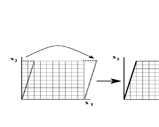
Figure 3: Two-dimensional representation of a plastic deformation, in which a piece of the undeformed volume is cut and then pasted in a different position.

A plastic deformation can be described by the “cut and paste” procedure depicted in Fig. 3, where pieces of matter are removed from one side and pasted on the opposite side of $\Delta V$ to obtain a compact but deformed volume element. We see that this procedure does not change the lattice structure. In this process pieces have been moved from one place to another in the volume, so that they have new neighboring pieces.

The use of this procedure was introduced by Volterrabib:volterra (quoted by Nabarro in Ref. nabarro67, ) in a paper devoted to the study of elastic deformations of multiply connected, three-dimensional bodies. The different constructions of the Volterra procedure lead to different kinds of defects. These ideal procedures can be performed on all the elementary volumes $\Delta V$ that compose the body. After the deformation, we may have two different situations: the deformed elements fit perfectly or they do not. In the latter case, we must apply a further deformation to re-compact the body. In the first case, we speak of a compatible deformation, in the second we have an incompatible deformation. Naively, a body remains compact (non-compact) if the deformation is compatible, while it changes its compactness (connectedness) state, if it undergoes an incompatible deformation.

Mathematically, an incompatible deformation corresponds to the non-integrability of the differential form $du^{i}$, which means that the displacement field $u^{i}(x)$ is multivalued, and thus that discontinuities arise when passing from one elementary volume element to another. This fact is expressed by,

$$\epsilon^{ikl}\partial_{k}\partial_{l}u^{j}=\alpha^{ij}\neq 0,$$ (5)

where $\epsilon^{ijk}$ is the completely antisymmetric tensor of rank three.

On the other hand, when the field is integrable, we have $\epsilon^{ikl}\partial_{k}\partial_{l}u^{j}=0$, and the deformation is described by a displacement field well defined in the entire body. Equation (5) says that a body is in an incompatible state when there is a “source of incompatibility” as represented by the tensor $\alpha_{ij}$ (see Ref. bib:kron, ).

These arguments help us understand the concept of a defect. The Volterra processes are just mental experiments, useful to explain and visualize incompatibility. A body may exist in an incompatibility state provided that there are defects in its structure, which are the sources of the incompatibility. For instance, the $\alpha_{ij}$ tensor appearing in Eq. (5) is called the density of dislocations, which are defects as described below.

We want to stress that the incompatibility state of the body should not be thought of as a result of a deformation used as a visualization tool. Rather, the incompatibility state is the result of the presence of defects in the structure of the body. In this section and the following ones, we shall often speak of incompatible deformations that correspond to a “defect state” of the medium. Nevertheless, this defect state should not be interpreted to be the result of an action on the body by an external agent. The concept of an incompatible deformation has been introduced because it is useful to understand the effects of the presence of defects. That is, when a body is filled with defects, its structure is similar to the one that can be reached due to the cut and paste procedure which we have introduced.

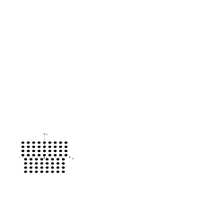
Figure 4: An “extra” half plane is inserted in the lattice, whose cross section is represented; the $z$ axis coincides with the line of the edge dislocation.

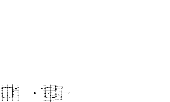
Figure 5: Burgers vector: on the left a path $B$ in the undeformed medium and, on the right, the correspondent path $B$ in the deformed medium: for each step along a lattice direction in the undeformed medium, a corresponding step is made in the deformed medium. The $z$ axis is the dislocation line.

We now will introduce in more detail some examples of defects and their corresponding mathematical characterization. The essential idea of a dislocation is geometric, and it can be illustrated by a simple argument.bib:landa7 Let us imagine that an extra half plane is inserted into a lattice whose cross section is represented in Fig. 4. The $z$ axis coincides with the edge of the half plane that has been introduced and is called an edge dislocation (the $z$ axis is called a dislocation line). In the neighborhood of the dislocation, the lattice planes fit together in an almost regular manner. The presence of defects causes a rearrangement of the whole structure, and the deformations exist even far from the dislocation. This far reaching rearrangement is easily evidenced if we consider any closed circuit of lattice points that encircles the dislocation line. If $\mathbf{u}$ is the displacement field that denotes the displacement of each point from its position in the ideal lattice, the total increment of this vector field around a circuit will not be zero, but it will be equal to a lattice spacing. Even though we have considered an edge dislocation only, the change in the displacement field is a general property of dislocations. After a round trip along any closed circuit that encloses a dislocation line, the displacement field increases by a vector which is called the Burgers vector of the dislocation. We can characterize mathematically the Burgers vector using Fig. 5, where an edge dislocation, which corresponds to removing a layer of lattice points, is depicted.footnote3 On the left, we have a closed path in the undeformed medium; on the right, the same path is traced in the deformed structure and shows the Burgers vector due to the presence of a dislocation. It is evident that, although the former path is closed, the latter is not. The deformation is defined by Eq. (1), which we write in discrete form

$$\mathbf{x}_{n}^{\prime}=\mathbf{x}_{n}+\mathbf{u}(\mathbf{x}_{n}),$$ (6)

where $n$ labels the nodes of the lattice. The difference between the position of the material points, as a consequence of a small deformation, can be written in the form,

$$\delta\mathbf{x}_{n}=\delta\mathbf{u}_{n},$$ (7)

as a function of the small displacement field $\delta\mathbf{u}_{n}$.

The closure gap is characterized by the Burgers vector $b^{i}$, which is defined by,

$$\sum_{n=1}^{N}\delta u^{i}_{n}=\sum_{B}\delta u^{i}_{n}=b^{i},$$ (8)

where $N$ is the total number of steps in the closed undeformed loop $B$ and $\delta u^{i}_{n}$ refers to the value of the displacement field in each step (see Ref. bib:klein89, ).

The mathematical meaning of the Burgers vector becomes clear when we pass to the continuous limit by letting the lattice spacing go to zero. In this limit Eq. (8) becomes

$$\oint_{B}du^{i}\equiv\oint_{B}\frac{\partial u^{i}}{\partial x^{j}}dx^{j}=b^{i}.$$ (9)

Equation (9) makes an explicit correspondence between the integrability properties of the differential form $du^{i}$ when dislocations are present and the Burgers vector and is independent of the structure of the lattice within the path $B$. The Burgers vector depends only on the fact that the path encloses a defect line.bib:kron

It is easy to see the dependence of the Burgers vector on the density of dislocations. If we use Eqs. (5) and (9) and Stokes’ theorem, we obtain

$$db^{h}=\alpha^{nh}dA_{n},$$ (10)

where $dA^{n}$ is the axial vector of the infinitesimal area element enclosed by the path $B$.

The structure of the medium is locally undeformed and to detect the presence of defects, a Burgers circuit is needed, which is a global procedure because it requires measurements in different places in the medium. The same holds for disclinations (see below). This fact will have an interesting interpretation when we describe defects in terms of geometrical properties, introducing torsion and curvature. By analogy, these are not seen locally, but appear when parallel transporting vectors in a differential manifold endowed with a suitable affine connection. Indeed, locally, the geometry always can be chosen to be flat.

Dislocations break the translational symmetry of the medium, while disclinations break its rotational symmetry. It is easy to understand what a disclination is if we perform the following Volterra process. Start from the disk-like medium depicted in Fig. 6. We remove a small slice, and then we unite the opposite faces along the cut. In this way, we obtain a medium that has an ordered structure everywhere except along the cut surface (the medium appears locally undeformed), where the displacement field is non-continuous. Mathematically a discontinuity appears, which corresponds to a wedge disclination.

The discontinuity $\Delta u^{i}$ of the displacement field is characterized by introducing a rotation vector $\Omega^{i}$ (Frank’s vector) parallel to the line $L$:

$$\Delta u^{i}(\mathbf{x})=(\mathbf{\Omega}\wedge\mathbf{x})^{i}.$$ (11)

This description is meaningful if the wedge is small, that is, if we adopt a linear theory. For disclinations, the ”linearity” condition is a very important issue, because if we want to introduce a density of disclinations and the corresponding Frank vectors, we must be able to sum these vectors to obtain the resultant one. As is well know, we cannot sum finite rotations in a straightforward way, because they do not commute. So we can define a density of disclinations provided that we confine ourselves to a linear theory, where the rotations described by the Frank’s vector are infinitesimal and can be summed without ambiguity.

The disclination density corresponding to each line is given by

$$\Theta_{ij}(\mathbf{x})=\delta_{i}(L)\Omega_{j},$$ (12)

where $\delta_{i}(L)$ is a Dirac delta function which is nonzero only along the disclination line $L$.bib:klein89

Volterra processes lead to six kinds of configurations, which belong to the six degrees of freedom of the proper group of motion in $\mathbb{R}^{3}$, that is, the Euclidean group defined by the semidirect product $SO(3)\otimes_{S}T(3)$. Hence, deformations resulting from the translational subgroup $T(3)$ are dislocations, while those belonging to the rotational subgroup $SO(3)$ are disclinations. As we shall see, this construction can be extended from 3 to $3+1$ dimensions, that is, by passing from Euclidean space to space-time.

Now we can link the concept of incompatibility to the density of defects in the medium. The presence of defects modifies the geometry of the medium. For example, as we see in Eq. (2), the distance between two physical points is different when a deformation is present. Moreover, we know that a deformation is the manifestation of the defects inside the medium, which corresponds to an incompatibility state. De St. Venantbib:dsv (quoted in Ref. bib:kron, ; see also Ref. tt, for a thorough review) showed that when a medium is in a state of compatible deformation, the following condition is fulfilled by the strain tensor $\varepsilon_{ij}$

$$\epsilon^{ikm}\epsilon^{jln}\partial_{k}\partial_{l}\varepsilon_{mn}=0.$$ (13)

In this case, the differential form $du^{i}$ is integrable, the displacement field $u^{i}(x)$ is well defined in the entire medium, and the strain tensor is its symmetric gradient (see Eq. (4)). On the other hand, when defects are present, Eq. (13) becomes

$$\epsilon^{ikm}\epsilon^{jln}\partial_{k}\partial_{l}\varepsilon_{mn}=\chi^{ij},$$ (14)

and the strain is said to be incompatible with the defects. The latter are characterized by the total density of defects tensor $\chi^{ij}$; moreover, $du^{i}$ is not integrable, and the displacement field is multivalued. The density of defects $\chi^{ij}$ is expressed in terms of the density of dislocations $\alpha_{ij}$ and the disclinations $\Theta_{ij}$ by the following relation (see, for example, Ref. bib:klein89, ):

$$\chi^{ij}\equiv\Theta^{ji}-\epsilon^{jmn}\partial_{m}(-\alpha^{i}_{n}+\frac{1}{2}\delta^{i}_{n}\alpha^{k}_{k}).$$ (15)

By means of eqs. (13), (14), (15) we have outlined the mathematical definition of defects. However, Eqs. (13)–(14) also have a more intuitive and physical interpretation. The total density of defects, $\chi_{ij}$, influences the state and the geometric properties of the medium. So we can think of $\chi_{ij}$ as a source term in a constitutive equation. In the following we shall see how this approach and the related definitions correspond to ECT.

For our purposes, we are interested in the geometrical description of the equilibrium state of a medium filled with defects, and we shall not study how stresses are linked to strains by a generalized Hooke’s law. In other words, we shall not consider the elastic reaction of the medium to the presence of defects. However, this problem is very interesting and consists in determining the stresses and strains of a given medium when the distribution of defects in it is given. It is worth mentioning that this internal problem of equilibrium is solved by a very elegant theorybib:kron58 that is based on the analogy between electromagnetism and the theory of defects. In Appendix B we shall describe this analogy in more detail, because we think that it would be of pedagogical interest to compare the mathematical structure of the fundamental equations of the two theories.

III Geometry of Defects

We want to see how defects influence the geometric structure of the medium. Equation (1) states the relation between the cartesian coordinates $x^{i}$ of a physical point in the medium and the new cartesian coordinates ${x^{\prime}}^{i}$ after the deformation. This correspondence is of the form ${x^{\prime}}^{i}={x^{\prime}}^{i}(x^{j})$. The change in the distance described in Eq. (2) can be thought of as a change in the metric tensor $g_{ij}$, which defines the distances between the physical points. In terms of the metric tensor we can write

$$dl^{2}=g_{ij}dx^{i}dx^{j}\rightarrow d{l^{\prime}}^{2}=g^{\prime}_{ij}dx^{i}dx^{j}.$$ (16)

From Eq. (2) we obtain

$$g_{ij}\rightarrowtail g^{\prime}_{ij}=g_{ij}+2\varepsilon_{ij}.$$ (17)

In this description, the coordinates of each physical point of the medium, before and after the deformation, are referred to a cartesian system of coordinates, which constitutes the background of the deformation. The coordinate lines of this system coincide with the lattice of the medium before the deformation, but things are different when the deformation has taken place.

This point of view is typical of a hypothetical external observer who is able to measure distances between two physical points of the medium and can confront the changes that occur with respect to a fixed external background. However, the distances can change not only because of the presence of defects, corresponding to an incompatible deformation. An external observer is able to notice the change even when the deformation is compatible (such is the case for a global dilatation). The external point of view is misleading, because the change in the metric is not directly linked to the presence of defects. It is more convenient to use a more intrinsic, that is, geometric point of view.

A compatible deformation can be described using another set of coordinates. Let us imagine that during the deformation the coordinates are dragged with the medium. Each particle of the medium is identified by a triplet of coordinates that does not change during the deformation. This identification is expressed by

$$y^{k^{\prime}}\,\hat{=}\,\,\delta_{k}^{k^{\prime}}x^{k},$$ (18)

which means that in the new system of coordinates, each particle has the same coordinates that it had before in the the ordered lattice. These coordinates are called “intrinsic”(see Ref. bib:kron, ).

An “internal” observer measures distances and labels and counts particles. Nothing changes when the number of particles does not change and the labelling is the same, as expressed by Eq. (18). The internal observer uses the coordinates $y^{k^{\prime}}$ as if they were Euclidean, although they are, in general, curvilinear if referred to the external cartesian background.

Things are different for an incompatible deformation. The internal observer notices a change in the number of particles along a round trip in the medium. There are excess holes or particles, and the labelling is not as simple as in Eq. (18). These intrinsic coordinates, together with the point of view of an internal observer, are useful for finding an incompatible deformation, that is, the presence of defects. The new and interesting thing is that the point of view of the internal observer suggests that we follow a purely geometric approach for describing the state of the medium. We shall see that the presence of defects is seen by the internal observer in terms of a change in the geometric properties of the medium. The internal geometry will no longer be Euclidean.

The intrinsic view suggests that relations can be found between the geometric properties of the medium (thought of as a differential manifold) and the densities of defects that influence them. These relations must be tensorial, that is, they must have a coordinate-independent meaning.

Suppose that our internal observer can perform measurements, that is, she has standard rods, and, moreover, is a good geometer: she knows how to transport rods and, in general, vectors and tensors in the medium. The result of the parallel transport of a vector $v^{h}$ along an infinitesimal displacement $dx^{m}$ is an infinitesimal change in the vector itselfbib:ruffi :

$$dv^{h}=-\Gamma_{ml}^{h}v^{l}dx^{m},$$ (19)

where $\Gamma_{ml}^{h}$ are the connection coefficients. In the absence of defects, the medium is Euclidean and cartesian coordinates are used and the connection coefficients are zero, while if there are defects, the observer notices that the “space of the medium” is not Euclidean, because the result of parallel transport along a closed contour is not zero. We want to link this idea to a geometric object, that is a tensor, so that its properties will not depend on the specific choice of the coordinates in the medium, but they will represent a real geometric structure. It is clear that the connection coefficients are somehow related to the defects, and the easiest way to see this relation is to give a new interpretation of the Burgers vector that we introduced before.

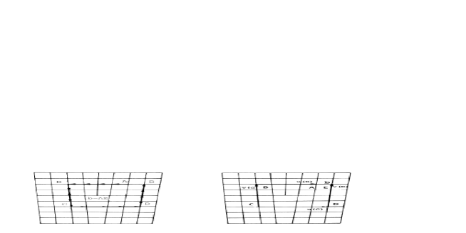
Figure 7: Dislocations and geometry: (a), on the left the usual Burgers circuit around an edge dislocation and; (b), on the right, the differential geometric view in terms of parallel transport.

In Fig. 7(a) we see the closure around a dislocation line represented by the Burgers vector. In Fig. 7(b) we see a different procedure, which has an intrinsic geometric meaning.bib:kron The vectors $\mathbf{u}(B)$ and $\mathbf{v}(D)$ are obtained, respectively, by parallel transporting $\mathbf{u}(C)$ along $\mathbf{v}(C)$ and $\mathbf{v}(C)$ along $\mathbf{u}(C)$. The gap we obtain is the Burgers vector. This procedure can be described using a continuous approach if we use the infinitesimal vectors $d_{1}x^{h}(C)$ and $d_{2}x^{h}(C)$ (1 and 2 refer to the coordinate lines, so that $\mathbf{u}(C)$ is parallel to direction 1 and $\mathbf{v}(C)$ is parallel to direction 2). By parallel transporting, we obtain

$$d_{1}x^{h}(B) = d_{1}x^{h}(C)-\Gamma_{ml}^{h}d_{1}x^{l}d_{2}x^{m}$$ (20a)

$$d_{2}x^{h}(D) = d_{2}x^{h}(C)-\Gamma_{ml}^{h}d_{2}x^{l}d_{1}x^{m},$$ (20b)

and the closure gap is

$$d_{2}x^{h}(C)+d_{1}x^{h}(B)-d_{1}x^{h}(C)-d_{2}x^{h}(D)=\Gamma_{ml}^{h}dA^{ml},$$ (21)

where $dA^{ml}=d_{1}x^{m}d_{2}x^{l}-d_{1}x^{l}d_{2}x^{m}$ is the antisymmetric tensor associated with the area delimited by these vectors. Because of the antisymmetry of $dA^{ml}$, the symmetric part of the connection coefficient is excluded in Eq. (21), and the remaining antisymmetric part, $S_{ml}^{h}=\Gamma_{[ml]}^{h}$, is called the torsion tensor. Note that the connection coefficients are not tensors, while their antisymmetric part is a tensor. From the relation

$$db^{h}=S_{ml}^{h}dA^{ml},$$ (22)

we can interpret $db^{h}$ as the infinitesimal closure defect (or the infinitesimal Burgers vector), and relate it to the torsion tensor. Equation (10) can be written in the form

$$db^{h}=\frac{1}{2}\alpha^{nh}e_{nml}dA^{ml}\doteq\alpha_{ml}^{h}dA^{ml},$$ (23)

where $e_{nml}$ and $e^{nml}$ are defined in terms of the completely antisymmetric tensors $\epsilon_{nml},\epsilon^{nml}$, and the determinant of the metric $g$:

$$e_{nml}=\sqrt{g}\epsilon_{nml}\,\ e^{nml}=\frac{1}{\sqrt{g}}\epsilon^{nml}.$$ (24)

If we compare Eqs. (22) and (23), it is easy to obtain

$$S_{ml}^{h}=\alpha_{ml}^{h}.$$ (25)

The meaning of Eq. (25) is that dislocations, through their density $\alpha_{ml}^{h}$ (defined in Eq. (23)), constitute the sources for torsion. This result is very general, and does not depend on the coordinates we used, because torsion is a tensor.

We have learned how dislocations modify the geometry of the medium, but dislocations are not the only effect of defects. The curvature of the medium also is influenced by the presence of defects. From a geometric point of view, it is known that in the presence of curvature, a vector undergoes a nonzero change when parallel transported along a closed path.bib:klein89 If the path is small and encloses a small surface characterized by $\Delta A^{nm}$, the change of the vector $v^{h}$ is given by

$$\Delta v^{h}=-\frac{1}{2}R_{nml}^{h}\Delta A^{nm}v^{l},$$ (26)

where $R_{nml}^{h}$ is the curvature tensor, which is antisymmetric in the $nm$ couple of indices.

Both torsion and curvature are manifested when parallel transport in the manifold is performed. They are global properties because locally the space can always be assumed to be flat. Generally speaking, we can imagine that, in the presence of defects, there is a source term for the curvature tensor

$$R_{nml}^{h}=\Theta_{nml}^{h},$$ (27)

but the meaning of the curvature in the theory of defects is more understandable if we use the (three-dimensional) Einstein tensor $G_{ij}$, which is a contraction of the curvature tensor

$$G^{ij}\equiv\frac{1}{4}e^{inm}e^{jlq}R_{nmlq}.$$ (28)

Moreover, in a linear theory of defects (see Sec. II), it is easy to show that the incompatibility equation (14) can be written as

$$\chi^{ij}=G^{ij}-\partial_{k}\epsilon^{jkl}k_{l}^{i},$$ (29)

where

$$k_{l}^{i}=(-\alpha_{l}^{i}+\frac{1}{2}\delta_{l}^{i}\alpha^{n}_{n}).$$ (30)

If we put the source terms on the same side, we can also write Eq. (29) as

$$G^{ij}=\sigma^{ij},$$ (31)

where $\sigma^{ij}=\chi^{ij}+\partial_{k}\epsilon^{jkl}(-\alpha_{l}^{i}+\frac{1}{2}\delta_{l}^{i}\alpha^{n}_{n})$.

We have introduced dislocations and disclinations, both from a mathematical and pictorial point of view. We then described the state of the medium by means of differential geometry and, finally, we have related the geometric properties of the medium to the defects, which are sources for the nontrivial structure of the continuum we consider. The next step is to study the correspondence with ECT, but before doing so, we must review this theory.

IV The Einstein-Cartan Theory of Gravitation

In the general theory of relativity, gravitation is explained in terms of the geometric properties of space-time. Space-time itself is seen as a dynamical object whose structure is determined by the energy-momentum distribution, and which determines the motion of the bodies contained in it.

To stress the role of geometry, Wheeler called the general theory of relativity “geometrodynamics.”bib:MTW Up to now, Einstein’s theory, besides having an intrinsic elegance, has satisfied all the observational tests (see Ref. bib:will, ), so that it is the classic and commonly accepted theory of gravitation. The effects of gravitation are determined by mass and its motion only in the form of energy and momentum. Of course, energy of different origin, such as electromagnetic energy, also influences the geometry of space-time. The constituents of macroscopic matter are elementary particles, which obey, at least locally, quantum mechanics and special relativity. As a consequence, elementary particles can be classified by the irreducible unitary representations of the Poincaré group and can be labelled by mass and spin. However, spin has no role in general relativity, that is, spin does not influence the geometry of space-time. This lack of influence is not a surprise if we confine ourselves to the study of macroscopic distributions of matter. Although mass has a monopole character (which is additive), spin is dipolar, and its effects are macroscopically zero, or averaged to zero (we are speaking of unpolarized spins). But this lack of influence is not completely satisfactory, because it is not clear why the spin cannot have a role in determining the geometry of the space-time continuum. Moreover, it cannot be excluded that, at the microscopical scale, spin could play a role.

The task of finding an agreement between a theory of gravitation, such as general relativity, and the theory of elementary particles, to obtain a quantum theory of gravitation, is one of the current problems of research. From a purely geometric point of view, general relativity can be amended to include spin to determine the properties of space-time. This is done in the Einstein-Cartan theory, which is based on a generalization of the geometric structure of general relativity. The Riemannian curvature was generalized in the 1920’s by Cartan,bib:cartan22 ; bib:cartan86 who introduced torsion degrees of freedom. From the late 1950’s to the early 1960’s, the concept of torsion was included in the formulation of gravitation as a gauge theory of the Poincaré group by Kibblebib:kibble and Sciama.bib:sciama The theory of gravitation with torsion is called the Einstein-Cartan theory, and it is described extensively in Ref. bib:hehl76, , where it is shown that the ECT is the local gauge theory of the Poincaré group in space-time. Other details are worked out by Hehlbib:hehl73b ; bib:hehl74 and by De Sabbata and Gasperini.bib:gaspa A more recent review has been done by Hammond.bib:hammond We shall give a very introductory primer to this theory and stress the differences with Einstein’s theory.

Mathematically, ECT differs from general relativity because torsion and (not only) the metric shape the structure of space-time. Physically, the presence of torsion is determined by the intrinsic spin of matter. Although energy-momentum is coupled to the metric tensor (and hence to curvature), spin is coupled to torsion. We have illustrated the geometric intuitive meaning of torsion, which is related to the closure gap of parallelograms. Now we have to transpose everything to four dimensions, but the idea remains the same. In the Einstein-Cartan theory of gravitation, space-time is defined as a semi-Riemannian manifold, endowed with a connection compatible with the metric, called a Riemann-Cartan space ($U_{4}$). The general form of a connection compatible with the metric is,footnote4

$$\Gamma_{\alpha\beta}^{\gamma}=\{_{\alpha\beta}^{\gamma}\}+K_{\alpha\beta}^{\gamma},$$ (32)

where $\{_{\alpha\beta}^{\gamma}\}$ are the Christoffel symbols (which are symmetric in the lower indices) and $K_{\alpha\beta}^{\gamma}$ is the contortion tensor and is a linear combination of torsion tensors (see Ref. bib:hehl76, ). Because $K_{\alpha\beta}^{\gamma}$ is not symmetric in the lower indices, we see that the “gammas” in Eq. (32) are not symmetric, while they are symmetric in general relativity, where, in particular, they reduce to the Christoffel symbols.

Einstein’s field equations determine the structure of space-time, relating Einstein’s tensor $G_{\alpha\beta}$, which is a combination of the derivatives of the metric, to the energy-momentum tensor $T_{\alpha\beta}$:

$$G_{\alpha\beta}=\kappa T_{\alpha\beta},$$ (33)

where $\kappa=8\pi G/c^{4}$ is Einstein’s gravitational constant.

The presence of torsion introduces new degrees of freedom in ECT, so that we write two field equations:bib:klein89

$$G^{\alpha\beta}-\frac{1}{2}D^{*}_{\gamma}(P^{\alpha\beta\gamma}-P^{\beta\gamma\alpha}+P^{\gamma\alpha\beta}) = \kappa T^{\alpha\beta}$$ (34)

$$P_{\alpha\beta}^{\gamma} = \kappa\Sigma_{\alpha\beta}^{\gamma}.$$ (35)

where $D_{\gamma}$ is the covariant derivative, $D^{*}_{\gamma}=D_{\gamma}+2S_{\gamma}=D_{\gamma}+2S_{\gamma\lambda}^{\lambda}$, and $P_{\alpha\beta}^{\gamma}$ is the Palatini tensor ($\frac{1}{2}P_{\alpha\beta}^{\gamma}\equiv S_{\alpha\beta}^{\gamma}+\delta_{\alpha}^{\gamma}S_{\beta}-\delta_{\beta}^{\gamma}S_{\alpha}$).

In Eqs. (34) and (35), together with the energy-momentum tensor $T_{\alpha\beta}$, spin is introduced by the spin-current-density tensor $\Sigma_{\alpha\beta}^{\gamma}$. We see that Eq. (34) generalizes Eq. (33), while Eq. (35) is a new equation for torsion. It is interesting to note that Eq. (35) is an algebraic equation: torsion does not propagate far from its sources. It follows that the field equations reduce to Einstein equations in vacuum. Because practically all tests of general relativity are based on consideration of Einstein’s equations in empty space, there is no difference in this respect between general relativity and ECT: the latter is as viable as the former.

It is expected that differences are present inside a spin distribution, and it is interesting to evaluate when the effects of spin are comparable to the mass effects. To evaluate the spin effects, we write Eq. (34) in a different form:bib:hehl76

$$G^{\{\}\alpha\beta}=\kappa\widetilde{T}^{\alpha\beta},$$ (36)

where $G^{\{\}\alpha\beta}$ is the symmetric (that is, Riemannian) part of the Einstein tensor (see Appendix A), and $\widetilde{T}^{\alpha\beta}$ is an effective energy momentum tensor, which has the form (leaving indices aside):

$$\widetilde{T}=T+\kappa\phi^{2},$$ (37)

where $T$ is the usual energy momentum tensor and $\phi$ is a tensor expressing the contribution of spin. It is clear that the effects of torsion are comparable to those of curvature when $T\simeq\kappa\phi^{2}$. In particular, if the mass density is $\rho=nm$, where $n$ is the number density and $m$ is the particle mass, and $s=n\hbar/2$ is the spin density, we expect spin effects to be of the same order as the mass effects when $\bar{n}\simeq m/\kappa\hbar^{2}$, or, alternatively, when the matter density is $\simeq 10^{47}$ g cm^-3 for electron-like matter and $10^{54}$ g cm³ for nucleon-like matter.bib:hehl76 These are extremely high densities, which are never reached in normal situations, even in extreme astrophysical objects. However, while in normal conditions the effects of torsion are completely negligible, they are expected to be important in cosmology.

Trautmanbib:traut99 introduced a characteristic length to estimate the effects of torsion, the “Cartan” radius. To achieve the condition $\rho\simeq\kappa s^{2}$, we can imagine that a nucleon of mass $m$ should be squeezed so that its radius coincides with the Cartan radius $r_{\rm Cart}$:bib:traut99

$$\frac{m}{r^{3}_{\rm Cart}}\simeq\kappa\bigl{(}\frac{\hbar}{r^{3}_{\rm Cart}}\bigr{)}^{2},$$ (38)

whence

$$r_{\rm Cart}\simeq(l^{*})^{\frac{2}{3}}(r_{\rm Compt})^{\frac{1}{3}},$$ (39)

where $l^{*}\simeq 1.6\times 10^{-33}$ cm is the Planck length, and $r_{\rm Compt}$ is the Compton length. For a nucleon we obtain $r_{\rm Cart}\simeq 10^{-26}$ cm, which is very small when compared with macroscopical scales, but it is larger than the Planck length. Hence, torsion must be taken into account to achieve a quantum theory of gravity.

Is it possible to detect the effects of torsion? As Hammondbib:hammond has carefully pointed out, the main task is to separate potential new torsion effects from the ones explained by known forces and fields. Moreover, even if from a geometric viewpoint torsion is well defined, there are various formulations of its generation from different sources, which make the search for the observed effects very difficult. To detect the effects of torsion, laboratory tests have been conceived such as trying to exploit an alignment of spin resulting in appropriate materials or studying the behavior of gyroscopes near torsion sources. On the large scale, there are possible implication of torsion on the evolution of the universe. For example, it has been shown that a spin fluid model could prevent the big bang singularity, even though at the same time, other models producing torsion would enhance the singularity (see Refs. bib:hehl76,  and bib:hammond, ). More recently, torsion has been incorporated in cosmic string theory, and as we shall point out, this way can be directly related to our analogy between the theory of defects and ECT. For a wide and careful analysis of torsion, both from a theoretical and experimental point of view, we refer to the excellent paper by Hammond.bib:hammond

V Comparison of the Theory of Defects and the Theory of Einstein-Cartan

In the previous sections we have outlined the main features of theory of defects and ECT. Now we will show the similarities and the differences between the two theories. Before we continue, we want to stress the underlying hypotheses that we assume. It is obvious that the two theories deal with different subjects, and we expect that any correspondence should be considered only as an analogy, and no more than that.

The basis of this analogy are the geometric methods that are used in both theories, because, although they are applied in a different geometric context, namely, the three-dimensional space for the theory of defects and the four-dimensional space-time for ECT, they both refer to continua. Thus, the two theories have a common formalism, and we look for analogies in the geometric objects that characterize the two theories. For instance, torsion plays a fundamental role in both theories.

The Einstein-Cartan theory is a geometric theory. Thus, we can use its field equations and geometric objects in a three-dimensional context. Consider the Einstein-Cartan field equations, Eqs. (34) and (35). In three (spatial) dimensions, they can be written using a linear approximation in the form:

$$G_{ij}-\frac{1}{2}\partial_{k}(P_{ij}^{k}-P_{j\,i}^{k}-P^{k}_{ij}) = \kappa T_{ij}$$ (40)

$$P_{ijk}\equiv 2S_{ijk}+2\delta_{ik}S_{j}-2\delta_{jk}S_{i} = \kappa\Sigma_{ijk}.$$ (41)

In three dimensions, $T_{ij}$ and $\Sigma_{ijk}$ coincide, respectively, with the force stress field and the moment stress field.

After a few calculations (see Ref. bib:klein89, ), it can be shown, using the relations between the torsion and dislocation density given in Eq. (25), that the field equation (41) becomes

$$P_{ijk}=\epsilon_{ijl}\alpha_{k}^{l},$$ (42)

which lets us identify the moment stress tensor with the density of dislocations: $\epsilon_{ijl}\alpha_{k}^{l}=\kappa\Sigma_{ijk}$. After similar calculations, the field equation (40) reduces to the incompatibility equation (29)

$$\chi^{ij}=G^{ij}-\partial_{k}\epsilon^{jkl}k_{l}^{i},$$ (43)

where $k_{li}$ has been introduced in Eq. (30). Equation (43) allows us to identify the total defect density tensor with the force stress tensor, $\chi_{ij}=kT_{ij}$.

Thus, we have seen that, formally, the Einstein-Cartan field equations describe the defect state of a three-dimensional continuum, at least when the defects are small so that we can use a linear approximation. The analogy is completed by the conservation equations, which, stated as geometric identities, give the correct conservation laws for dislocations and disclinations.

This analogy should not be surprising, because, as we said before, it is based on the common geometric structure of the two theories. In particular, it is evident that the comparison cannot be done with general relativity, where the torsion is zero.

Now we ask if we start from this three-dimensional correspondence in the linearized theory, is it possible to say something about the $3+1$ space-time situation? In other words, we want to investigate under what assumptions we can treat space-time as a defect state of a four-dimensional continuum. The bases of our investigation are the geometric analogies. Let us point out the main features of these analogies.

When passing from 3 to 4 dimensions, there is an important difference in the geometric description of the medium. In three dimensions we can say that the effect of disclinations is to produce curvature. We used the Einstein tensor $G_{ij}$ to write the incompatibility equation, but we did not say explicitly that the curvature tensor and the Einstein tensor are equivalent. It is well known that in three dimensions they have the same number of independent components, which means that when the curvature tensor is zero, the Einstein tensor also is zero and vice versa. The presence of defects produces a nontrivial Einstein tensor, which also means that the curvature tensor is not zero. The same correspondence does not hold in four (or more) dimensions, because we can have curvature even if the Einstein tensor is zero. In particular, far from the sources, the curvature tensor could be nonzero. Indeed, this happens also in general relativity, because space-time is curved even far from the sources.

If we extend the analogy to a four-dimensional context, we should expect that the effects of defects propagate through the manifold and are not purely local, as in three dimensions.

Kleinert,bib:klein89 adopted a linearized approach and showed that space-time with torsion and curvature can be generated from a flat space-time using “singular coordinate transformations,” and is completely equivalent to a medium filled with dislocations and disclinations. In other words his singular coordinate transformations are the space-time equivalent of the plastic deformations which lead to incompatible states (see Sec. II). Hence, at least in this approximation, space-time can be thought of as a defect state, and defects are nothing but mass, mass current, and spin.

The next important point is to try to go beyond the linear approximation. We did our previous comparisons assuming small defects in order to use a linearized theory. As we have said, this assumption is fundamental for defining a density of disclinations. We must consider also that in real bodies there are physical constraints on the size of defects: additional or missing matter should not be such as to produce cracks in the structure. Hence, from a phenomenological point of view, it is often sufficient to use a linear theory, as it usually the case for the elastic theory of defects, where the linear Hooke’s law is used.

However, curvature and torsion can always be introduced geometrically by the parallel transport procedure that we outlined in Sec. III. No approximation is contained in the equations governing curvature and torsion, so from the viewpoint of a geometric treatment no linearization is needed.

If we keep in mind the differences that arise when we pass from three to four dimensions, we can write four-dimensional equations which characterize the state of the medium:

$$G^{\alpha\beta} = \sigma^{\alpha\beta}$$ (44)

$$S_{\alpha\beta}^{\gamma} = \alpha_{\alpha\beta}^{\gamma}.$$ (45)

As we show in Appendix A, Eq. (44) is equivalent to a nonlinear generalization of the incompatibility equation, and Eq. (45) states the proportionality between torsion and the dislocations tensors. In a three-dimensional context these equations are equivalent respectively to Eqs. (40) and (41), and they can be interpreted as constitutive equations. In other words, Eqs. (44) and (45) determine the geometric structure of the medium once the sources are given.

Now it is easy to compare these equations to the Einstein-Cartan field equations written in the form:

$$G^{\alpha\beta} = \kappa\Psi^{\alpha\beta}$$ (46)

$$P_{\alpha\beta}^{\gamma} = \kappa\Sigma_{\alpha\beta}^{\gamma},$$ (47)

where $\Psi^{\alpha\beta}$ is defined by

$$\Psi^{\alpha\beta}\equiv T^{\alpha\beta}+\frac{1}{2}D^{*}_{\gamma}(\Sigma^{\alpha\beta\gamma}-\Sigma^{\beta\gamma\alpha}+\Sigma^{\gamma\alpha\beta}).$$ (48)

The correspondence between Eqs. (47) and (45) is obtained using the definition of the Palatini tensor given in Sec. IV.

We can then say that Einstein-Cartan space-time can be considered as a defect state of a four-dimensional continuum, and the equations that describe the dynamical properties of this continuum correspond to the incompatibility equation and torsion source equation for space-time. This correspondence is an interesting analogy for the Einstein-Cartan theory.

The meaning of the analogy becomes clear on physical grounds when we use three-dimensional equations in a linear theory of defects, where we have seen that the dislocation density is analogous to the moment stress tensor, and the total density of defects is analogous to the force stress tensor.

V.1 Space-Time Defects and cosmic strings

The approach that we have outlined has been investigated more formally by Puntigam and Soleng,bib:puntigam who exploited the analogy between the theory of defects and ECT in the field of cosmic strings. The latter are topological space-time defects and are similar to the line-like dislocations and disclinations in three-dimensional space which carry torsion and curvature.

Exploiting the above analogy and generalizing the Volterra processes to $3+1$ dimensions, “distorted space-times” are built in the paper by Puntigam and Soleng, starting from a Minkowski space-time. In this analogy, the Poincaré group, which is defined by the semidirect product $P(10)=SO(1,3)\otimes_{S}T(4)$, takes the place of the Euclidean group of $\mathbb{R}^{3}$. In this case we have six kinds of disclination-like deformations, and four kinds of dislocation-like deformations, which yield 10 different Riemann-Cartan spaces filled with topological defects.

In this generalization, distorted space-times are locally undeformed, just as in the three-dimensional case (see Sec. II), but in order to detect the effect of space-time defects, it is possible to use a procedure similar to the one that led to the definition of the Burgers and Frank vectors. Without going into detail, we only mention that a Burgers vector $\mathbf{B}\in T(4)$ and a Frank matrix $\mathcal{G}\in S(1,3)$ are defined by the parallel transport of a tetrad in the Riemann-Cartan space $U_{4}$ around the line-like defect region. In this way, a space-time with curvature and torsion is thought of as a distorted medium filled with dislocations and disclinations, and it is shown that the matter distributions, which in the Einstein-Cartan theory act as sources, can be interpreted as cosmic strings and cosmic dislocations. The analogy that we have described seems promising for the study of such objects.

VI Summary

The Einstein-Cartan theory of gravitation has been introduced starting from an analogy with the static theory of defects, which describes the equilibrium state of a three-dimensional continuum. By introducing the fundamental equations of the Einstein-Cartan theory, we recalled that it agrees with the known tests of general relativity. Moreover, we stressed that the Einstein-Cartan theory has a richer geometric and physical structure. In particular, a non-symmetric connection is used, and torsion is linked to the density of spin. In ECT, both the mass and spin determine the geometric properties of space-time and shape its structure.

We also showed that in the classical theory of defects, a geometric approach is possible and leads to the description of a continuous medium by means of geometric entities that are determined by the presence of defects, such as disclinations and dislocations which we related to curvature and torsion. Then we outlined a comparison between these two theories, which share a similar underlying geometric structure, even though they apply to very different physical phenomena.

We showed that the equations that describe the state of the medium and its structure in the presence of defects may be interpreted as the Einstein-Cartan field equations for a three-dimensional continuum, at least in the linear approximation. On the other hand, the incompatibility equation of the theory of defects, which is usually obtained in the linear approximation, can be extended to a more general situation, where defects are not necessarily assumed to be small.

By pursuing this formal analogy, space-time, as described by ECT, can be interpreted as a defect state of a four-dimensional continuum. We suggest that this analogy, although formal, might be useful in modern astrophysics, because cosmic strings may be interpreted as extensions of three-dimensional defects.

It is fascinating that the theory of defects, whose origin dates back to the beginning of the 20th century, can have such a strong and fruitful analogy with recent developments in theoretical physics. We believe that the analogy we have outlined can be useful for understanding the key concepts of differential geometry and the geometric theories of gravitation as well as helping to stimulate interest in these fields.

Appendix A Nonlinear generalization of the incompatibility law

It is easy to generalize the incompatibility equation (14) on purely geometric grounds, extending the definition given in the linear approximation to a general relation. We define

$$R_{nml}^{k}=\partial_{n}\Gamma_{ml}^{k}-\partial_{m}\Gamma_{nl}^{k}+\Gamma_{np}^{k}\Gamma_{ml}^{p}-\Gamma_{mp}^{k}\Gamma_{nl}^{p},$$ (49)

as the curvature tensor associated with the connection $\Gamma_{ij}^{k}$. We obtain the Riemann tensor $R_{nml}^{\{\}k}$, which consists of the purely symmetric part of the connection, and which is obtained from Eq. (49) by substituting the Christoffel symbols $\{_{ij}^{k}\}$ into the connection coefficients $\Gamma_{ij}^{k}$. As we recalled in Sec. IV, the general form of the connection compatible with the metric in the Riemann-Cartan spaces is

$$\Gamma_{jk}^{i}=\{_{jk}^{i}\}+K_{jk}^{i},$$ (50)

and although the Christoffel symbols are symmetric in the lower indices, the contortion tensor $K_{jk}^{i}$ is not, and hence the connection is no longer symmetric.

If we start from Eq. (49), it is straightforward to obtain the symmetric part of the Einstein tensor $G^{\{\}ij}$. Because in the linear approximation, the incompatibility tensor is related to the symmetric part of the Einstein tensor,bib:klein89

$$G^{\{\}ij}\equiv\epsilon^{ikl}\epsilon^{jmn}\partial_{k}\partial_{m}\varepsilon_{ln},$$ (51)

the natural extension of the incompatibility equation (14) can be performed using Eq. (51).

The source equation for the Einstein tensor,

$$G^{ij}=\sigma^{ij},$$ (52)

is written in the form,

$$G^{ij}\equiv G^{\{\}ij}-\eta^{ij}-\psi^{ij}=\sigma^{ij},$$ (53)

where

$$E_{jkl} = \frac{1}{2}(\partial_{j}\varepsilon_{kl}+\partial_{k}\varepsilon_{jl}-\partial_{l}\varepsilon_{jk})$$ (54a)

$$\eta^{ij} \equiv -\frac{1}{2}e^{inm}e^{jlq}\partial_{n}K_{mlq}$$ (54b)

$$\psi^{ij} \equiv \frac{1}{2}e^{inm}e^{jlq}g^{kp}(2E_{nqk}K_{mlp}+2E_{mlp}K_{nqk}+K_{nqk}K_{mlp})$$ (54c)

(see Ref. bib:gai, ). Moreover, $G^{\{\}ij}$ can be written as

$$G^{\{\}ij}=e^{inm}e^{jlq}\partial_{n}\partial_{l}\varepsilon_{mq}-2e^{inm}e^{jlq}g^{kp}E_{nqk}E_{mlp},$$ (55)

and if we write $\Xi^{ij}=2e^{inm}e^{jlq}g^{kp}E_{nqk}E_{mlp}$, Eq. (53) becomes

$$e^{inm}e^{jlq}\partial_{n}\partial_{l}\varepsilon_{mq}-\Xi^{ij}-\eta^{ij}-\psi^{ij}=\sigma^{ij},$$ (56)

which is the desired extension of the incompatibility equation. We obtain the usual relation if we notice that $\Xi^{ij}$, $\eta^{ij}$, and $\psi^{ij}$ are nonlinear contributions.

Although we obtained Eq. (56) for three dimensions, our approach is based entirely on geometric foundations and can be easily transposed into curved space-time, which, in this sense, can be interpreted as an incompatibility state.

Appendix B Operators on symmetric tensors

We give a different and perhaps more intuitive, interpretation of some of the concepts we have introduced. Krönerbib:kron58 has developed a continuum theory of dislocations and disclinations using an approach that is very similar to electromagnetic theory. Equations that give internal stresses in terms of source functions (that is, defect densities) are formulated and are analogous to Poisson equations. To give an idea of this formalism, we show that the equations and the tensors that we introduced in the main text can be defined in a different way using the technique of differential operators on symmetric tensors (see Refs. bib:kron, and also bib:dewit, ).

We introduced the strain tensor in Eq. (4). A different definition may be given using the deformation operator def, which is a type of symmetric gradient:

$$\mathbf{\varepsilon}={\tt def}\,\mathbf{u}\Leftrightarrow\varepsilon_{ij}=\frac{1}{2}(\partial_{i}u_{j}+\partial_{j}u_{i}).$$ (57)

In the same way, an incompatibility operator inc may be introduced, by which the incompatibility equation reads

$${\tt inc}\,\mathbf{\varepsilon}=\mathbf{\chi}\Leftrightarrow\epsilon^{ikm}\epsilon^{jln}\partial_{k}\partial_{l}\varepsilon_{mn}=\chi^{ij}.$$ (58)

Finally, it is obvious that we may introduce a divergence operator div, whose meaning is well known:

$${\tt div}\,\mathbf{\varepsilon}\Leftrightarrow\varepsilon^{ij}_{,j}.$$ (59)

The point is that the tensor operators def, inc, and div are analogous to the vector operators grad, curl, and div. It is easy to verify that

$${\tt div}\,{\tt inc}\equiv 0\quad\mbox{and}\quad{\tt inc}\ {\tt def}\equiv 0,$$ (60)

which are the analogs of ${\tt div}\,{\tt curl}\equiv 0$ and ${\tt curl}\,{\tt grad}\equiv 0$.

As it is well known, a vector $\mathbf{v}$ that vanishes at infinity can be decomposed into a gradient of a scalar function $\varphi$ and the curl of a vector function $\mathbf{A}$:

$$\mathbf{v}={\tt grad}\,\varphi+{\tt curl}\,\mathbf{A}.$$ (61)

In the same way Kröner showed that a symmetric second rank tensor $\mathbf{T}$ that vanishes at infinity can be decomposed into two terms, that is, a deformation of a vector field $\mathbf{u}$ and the incompatibility of a symmetric second rank tensor $\mathbf{S}$:

$$\mathbf{T}={\tt def}\,\mathbf{u}+{\tt inc}\,\mathbf{S}.$$ (62)

Thus, if a symmetric tensor field has zero divergence, it can be written as a pure incompatibility field, while, if it has zero incompatibility, it can be written as a pure deformation field.

By starting from this analogy, Kröner was able to write the equations relating the internal stress and strain to the sources of incompatibility (the densities of defects). This procedure is analogous to the one that is used in electromagnetism, where the potential and fields are computed starting from the Poisson or Laplace equations. The electromagnetic analogy is very useful and provides a clear understanding of the problem of the link between defects and internal strain. Moreover the analogy recalls closely ECT, where the geometry of space-time is determined by the energy-momentum tensor and spin current tensor. Indeed, in Kröner’s approach, the strain of the medium, that is, its geometry, is determined by the distribution of defects.

Figure 1: Two-dimensional representation of the undeformed volume element $\Delta V$ and its lattice structure.

Figure 2: two-dimensional representations of elastic deformations, which result from tilt and stretching operations on the underformed volume element. Parts of the body that were close to each other remain close even after the deformation.

Figure 6: We obtain a wedge disclination removing a slice from the disk-like piece of medium, and then uniting the opposite faces along the cut. $L$ is the disclination line.

References

- (1) P. West, Introduction to Supersymmetry and Supergravity (World Scientific, Singapore, 1990).
- (2) In these sections we present the fundamental ideas of the theory of defects, with the aim of drawing a formal analogy with ECT. We shall follow the work of Kröner,bib:kron De Wit,bib:dewit Nabarro,nabarro67 Gairola,bib:gai and Kleinert.bib:klein89 References to earlier papers can be found in these papers.
- (3) E. Kröner, “Continuum theory of defects,” in Les Houches 1980, Session XXXV: Physics of Defects, edited by R. Balian, M. Kléman, and J. P. Poirier (North Holland, Amsterdam, 1980), pp. 215–315
- (4) R. De Wit, “The continuum theory of stationary dislocations,” edited by F. Seitz and D. Turnbull in Solid State Physics 10, 249–292 (1960).
- (5) F. R. N. Nabarro, Theory of Crystal Dislocations (Dover Publications, New York, 1967). A historical review of the theory of dislocations is given here.
- (6) B. K. D. Gairola, “Nonlinear elastic problems,” in Dislocations in Solids, edited by F. R. N. Nabarro (North Holland, Amsterdam, 1979), pp. 223–342.
- (7) H. Kleinert, Gauge Fields in Condensed Matter, Vol II: Stresses and Defects (World Scientific, Singapore, 1989).
- (8) Latin indices run from 1 to 3, and there is no need to distinguish between covariant and contravariant ones, because the background metric is Euclidean. However, we shall use covariant and contravariant indices in summations; in order to use the Einstein convention; means .
- (9) L. D. Landau and E. M. Lifshits, Theory of Elasticity (Butterworth-Heinem, New York, 1995).
- (10) V. Volterra, “Sur l’équilibre des corps élastiques multiplement connexes,” Ann. Éc. Norm. Sup. 24, 401–517 (1907).
- (11) The term defect refers both to a true absence of particles and to an excess of them, with respect to the ordered structure of the medium, which, according to common terminology, we shall call an undeformed medium.
- (12) A. J. C. B. St. Venant, Résumé des Leçons sur l’application de la Mécanique, par C.L.M.H. Navier, (Didot, Paris, 1864).
- (13) C. Truesdell and R. Toupin, “The classical field theories,” in Encyclopedia of Physics, edited by S. Flügge (Springer-Verlag, Berlin-Göttingen-Heidelberg, 1960), Vol. 3, Part 1, pp. 226–793.
- (14) E. Kröner, “Kontinuumstheorie der Versetzungen und Eigenspannungen”, in Ergebnisse der Angewandte Mathematik, Vol. 5, edited by L. Collatz and F. Lösch Springer-Verlag, Berlin-Göttingen-Heidelberg, 1958)
- (15) H. C. Ohanian and R. Ruffini, Gravitation and Spacetime (W. W. Norton and Company, New York, 1994).
- (16) C. W. Misner, K. S. Thorne, and J. A. Wheeler, Gravitation (Freeman, San Francisco, 1973).
- (17) C. M. Will, Theory and Experiment in Gravitational Physics (Cambridge University Press, Cambridge, 1993).
- (18) ’E. Cartan “Sur une généralisation de la notion de courbure de Riemann et les espace à torsion,” C. R. Acad. Sci. (Paris) 174, 593–595 (1922).
- (19) É Cartan, On Manifolds with an Affine Connection and the Theory of General Relativity, translated by A. Magnon and A. Ashtekar (Bibliopolis, Naples, 1986).
- (20) T. W. B. Kibble, “Lorentz invariance and the gravitational field,” J. Math. Phys. 2, 212–221 (1961).
- (21) D. W. Sciama, “On the analogy between charge and spin in general relativity,” in Recent Developments in General Relativity (Pergamon, Oxford, 1962), pp. 415–439
- (22) F. W. Hehl, P. Von der Heyde, G. D. Kerlick, and J. D. Nester, “General Relativity with spin and torsion: Foundations and prospects,” Rev. Mod. Phys. 48, 393–416 (1976).
- (23) F. W. Hehl, “Spin and torsion in general relativity: I. Foundations,” Gen. Rel. Grav. 4, 333–349 (1973).
- (24) F. W. Hehl, “Spin and torsion in general relativity: II. Geometry and field equations,” Gen. Rel. Grav. 5, 491–516 (1974).
- (25) V. De Sabbata and M. Gasparini, Introduction to Gravitation (World Scientific, Singapore, 1985)
- (26) T. A. Hammond, “Torsion gravity,” Rep. Prog. Phys. 65, 599–649 (2002).
- (27) Greek indices run from 0 to 3 and are raised and lowered by the metric tensor ; the signature of space-time is , and again, the summation convention is used.
- (28) A. Trautman, “Gauge and optical aspects of gravitation,” Class. Quan. Grav. 16, A157–A175 (1999).
- (29) R. A. Puntigam and H. H. Soleng, “Volterra distorsion, spinning strings, and cosmic defects,” Class. Quant. Grav. 14, 1129–1149 (1997).