Wormhole solutions in the Randall-Sundrum scenario

Abstract

In the simplest form of the Randall-Sundrum model, we consider the metric generated by a static, spherically symmetric distribution of matter on the physical brane. The solution to the five-dimensional Einstein equations, obtained numerically, describes a wormhole geometry.

I Introduction

In the last few years large extra dimensions and brane worlds have been the subject of intensive investigations. The situation can be simplified to a five-dimensional problem where matter fields are confined to the four-dimensional spacetime while gravity acts in five dimensions. If the extra dimension has a finite extension its compactification radius may be larger than the Planck length without conflict with observations [1]. Alternatively, the extra dimension may be kept warped and compactified or uncompactified [2,3] or even neither compact nor warped with a truly infinite size [4]. A considerable effort has been devoted in exploring possible phenomenological and observable consequences of the brane world scenario. In particular Lorentzian wormholes [5,6], smooth bridges connecting different universes or remote parts of the same universe, have gained much attention and have found a natural source in brane world models (see [7] and references quoted therein). In this letter we will show that a solution to Einstein equations in the Randall-Sundrum scenario with a mass point on the physical brane can describe a wormhole geometry. The paper is organized as follows. In Section II we start from the simplest form of the Randall-Sundrum model and modify the corresponding metric, which is asymptotically anti-de Sitter, to a metric generated by a static, spherically symmetric distribution of matter on the physical brane or, equivalently, axially symmetric in the bulk. By a suitable choice of coordinates we succeed in reducing the solution of the five-dimensional Einstein equations to the solution of a single ordinary differential equation in one unknown function. In Section III we solve numerically the highly nonlinear equation obtained and show that there are wormhole solutions in the brane world. Some concluding remarks are given in Section IV.

II The model

There are in fact two models due to Randall and Sundrum with essentially the same framework. In the RS1 model [2] we have two 3-branes with equal and opposite tensions which rigidly reside at the boundaries ($y=0$ and $y=r_{c}\pi$) of a slab of a five-dimensional anti-de Sitter bulk spacetime of radius $\ell$. The five-dimensional Einstein equations in the vacuum are

$$G_{AB}=R_{AB}-\dfrac{1}{2}g_{AB}R=-\,\frac{\Lambda}{4M_{5}^{3}}g_{AB}$$ (1)

Here $M_{5}$ and $\Lambda$ denote respectively the five-dimensional Planck scale and the (negative) bulk cosmological constant. The Randall-Sundrum solution to the previous equations is

$$ds^{2}=e^{-2k\,|y|}\,\eta_{\mu\nu}dx^{\mu}dx^{\nu}+dy^{2}$$ (2)

where $\eta_{\mu\nu}$ is the flat Minkowskian metric, and $k=\frac{1}{\ell}$ is a scale factor for the extra dimension $y$. The above solution holds only if the tensions of the branes and the bulk cosmological term are fine-tuned and in particular this implies that $k$ must take the value $k=\sqrt{-\dfrac{\Lambda}{24M_{5}^{3}}}$. Moreover the following relation is derived

$$M_{4}^{2}=\frac{M_{5}^{3}}{k}(1-e^{-2kr_{c}\pi})$$ (3)

which gives a well defined value for the 4D Planck scale $M_{4}$ even in the infinite radius limit. So if $M_{5}$ and $k$ are taken both of order $M_{4}$ and $kr_{c}\pi\approx 35$ the model suggests a solution to the hierarchy problem by showimg that TeV energy scales on the “TeV brane” at $y=r_{c}\pi$ correspond to $10^{16}$ TeV energy scales on the “Planck brane” at $y=0$. In an alternate scenario known as RS2 [3] the second brane, where now is supposed to be concentrated the graviton zero mode, is taken off at infinity letting $r_{c}\to\infty$, while the Standard Model particles are assumed to live on the brane at $y=0$. Such localization of gravity can obviate the need for the compactification of the fifth dimension. RS2 does not solve the hierarchy problem as RS1 does, but it is of interest from a purely gravitational point of view. While in the absence of matter the line interval can be exactly obtained, complications arise in the presence of matter fields, and even if an analytic expression could be found for the metric produced by a matter distribution on the physical brane it certainly would involve special functions, as one can see in linear and beyond linear order approximate solutions [8,9,10].

Here we assume for simplicity that the matter fields reduce to a point mass on the physical brane. Having in mind the four-dimensional McVittie solution [11], which represents the gravitational field of a mass particle in a Friedmann-Robertson-Walker universe and its generalization to higher dimensions [12], we employ similar methods to obtain a solution although the metric we are searching for is not spherically symmetric in five dimensions.

We start from the sourceless $AdS_{5}$ solution given by

$$ds^{2}=e^{-2k|y|}\,(dr^{2}+r^{2}d\Omega^{2}-dt^{2})+dy^{2}$$ (4)

where $d\Omega^{2}$ is the line element on a two-dimensional sphere of unit radius, and apply to it the following transformation of the Robertson type [13]

$$\begin{cases}r=&e^{kz}\,\dfrac{\rho}{\sqrt{1+k^{2}\rho^{2}}}\\ {}&\\ y=&z-\dfrac{1}{2k}\,\log{(1+k^{2}\rho^{2})}\end{cases}$$ (5)

so obtaining

$$ds^{2}=\dfrac{d\rho^{2}}{1+k^{2}\rho^{2}}+\rho^{2}d\Omega^{2}-e^{-2kz}\,(1+k^{2}\rho^{2})\,dt^{2}+(1+k^{2}\rho^{2})\,dz^{2}$$ (6)

In the presence of a point mass $m$ bound at $r=0$ to the physical brane in the old coordinates and consequently bound at $\rho=0$ in the new coordinates, we make the ansatz that the line element (6) becomes

$$ds^{2}=e^{\alpha(\rho)}\,d\rho^{2}+e^{\beta(\rho)}\,\rho^{2}d\Omega^{2}-\,e^{-\,2kz+\gamma(\rho)}\,dt^{2}+e^{\omega(\rho)}\,dz^{2}$$ (7)

In the above five-dimensional metric we used only four of the five available degrees of freedom, so (7) still has a degree of generality which can applied in future contexts. From Einstein equations (1), written in the mixed form

$$G_{A}^{B}=6k^{2}\delta_{A}^{B}$$ (8)

we obtain, omitting for simplicity the $\rho$-dependence

$$G_{t}^{z}=\dfrac{k}{2}e^{\,\omega}(\gamma^{\prime}-\omega^{\prime})=0$$ (9)

Therefore putting $\gamma=\omega$ one realizes by inspection that two of the components of the mixed Einstein tensor, namely $G_{t}^{t}$ and $G_{z}^{z}$, are equal.

Finally the relevant equations are

$$\dfrac{1}{4\rho^{2}}\{e^{-\alpha}[4-4e^{\alpha-\beta}+4e^{\alpha-\gamma}k^{2}\rho^{2}+\rho^{2}{\beta^{\prime}}^{2}+8r\gamma^{\prime}+\rho^{2}{\gamma^{\prime}}^{2}$$

$$\hskip 21.68121pt+4\rho\beta^{\prime}(1+\rho\gamma^{\prime})]\}=6k^{2}$$ (10a)

$$\dfrac{1}{4\rho}\{e^{-\alpha}[4e^{\alpha-\gamma}k^{2}\rho+\rho{\beta^{\prime}}^{2}+4\gamma^{\prime}+3\rho{\gamma^{\prime}}^{2}+2\beta^{\prime}(2+\rho\gamma^{\prime})$$

$$\hskip 21.68121pt-\alpha^{\prime}(2+\rho\beta^{\prime}+2\rho\gamma^{\prime})+2\rho\beta^{\prime\prime}+4\rho\gamma^{\prime\prime}]\}=6k^{2}$$ (10b)

$$\dfrac{1}{4\rho^{2}}\{e^{-\alpha}[-4e^{\alpha-\beta}+4+3\rho^{2}{\beta^{\prime}}^{2}+4\rho\gamma^{\prime}+\rho^{2}{\gamma^{\prime}}^{2}+2\rho\beta^{\prime}(6+\rho\gamma^{\prime})$$

$$\hskip 21.68121pt-\rho\alpha^{\prime}(4+2\rho\beta^{\prime}+\rho\gamma^{\prime})+4\rho^{2}\beta^{\prime\prime}+2\rho^{2}\gamma^{\prime\prime}]\}=6k^{2}$$ (10c)

Solving for $e^{\alpha}$ in equation (10a) and substituting this value into equations (10b) and (10c) we obtain:

$$e^{\alpha}=\dfrac{e^{\beta+\gamma}\,\left[\left(2+\rho\,\beta^{\prime}\right)\,\left(2+\rho\,\beta^{\prime}+4\rho\,\gamma^{\prime}\right)+\rho^{2}{\gamma^{\prime}}^{2}\right]}{4\,\left[e^{\gamma}+e^{\beta}\,\left(-\,1+6\,e^{\gamma}\right)\,k^{2}\rho^{2}\right]}$$ (11a)

$$\dfrac{3\gamma^{\prime}}{\left[\left(2+\rho\,\beta^{\prime}\right)\,\left(2+\rho\,\beta^{\prime}+4\rho\,\gamma^{\prime}\right)+\rho^{2}{\gamma^{\prime}}^{2}\right]}\,\Phi(\rho)=0$$ (11b)

$$\dfrac{3(2+\rho\beta^{\prime})}{\left[\left(2+\rho\,\beta^{\prime}\right)\,\left(2+\rho\,\beta^{\prime}+4\rho\,\gamma^{\prime}\right)+\rho^{2}{\gamma^{\prime}}^{2}\right]}\,\Phi(\rho)=0$$ (11c)

where

$$\Phi(\rho)=\,\,e^{-\beta}\rho\{\gamma^{\prime}[\rho[\rho{\beta^{\prime}}^{2}+4(\rho\gamma^{\prime}+1)\beta^{\prime}+\gamma^{\prime}(\rho\gamma^{\prime}+8)-2\rho\beta^{\prime\prime}]+8]$$

$$\hskip 43.36243pt+2\rho(\rho\beta^{\prime}+2)\gamma^{\prime\prime}\}-k^{2}\rho^{2}\{4[\rho[\rho^{2}{\beta^{\prime}}^{3}+3\rho(\rho\gamma^{\prime}+2){\beta^{\prime}}^{2}$$

$$\hskip 43.36243pt-3[\rho[\gamma^{\prime}(\rho\gamma^{\prime}-4)+\rho\gamma^{\prime\prime}]-4]\beta^{\prime}-\gamma^{\prime}[\rho[\gamma^{\prime}(\rho\gamma^{\prime}+6)-3\rho\beta^{\prime\prime}]-6]$$

$$\hskip 43.36243pt-6\rho\gamma^{\prime\prime}]+8]-e^{-\gamma}[\rho[\rho^{2}{\beta^{\prime}}^{3}+2\rho(2\rho\gamma^{\prime}+3){\beta^{\prime}}^{2}+[\rho[\gamma^{\prime}(\rho\gamma^{\prime}+16)$$

$$\hskip 43.36243pt-2\rho\gamma^{\prime\prime}]+12]\beta^{\prime}+2\gamma^{\prime}[\rho(\gamma^{\prime}+\rho\beta^{\prime\prime})+6]-4\rho\gamma^{\prime\prime}]+8]\}$$ (12)

Equation (11b) can be satisfied by $\gamma=0$, but in this case (11c) and (11a) become respectively $k^{2}=0$ and $e^{\alpha}=e^{\beta}(2+\rho\beta^{\prime})^{2}$ so it is immediate to verify, passing to standard coordinates, that we would have a flat five-dimensional space solution without cosmological constant. In the same way equation (11c) can be satisfied by $\beta=2\ln(\rho_{0}/\rho)$ but, apart the unpleasant fact that the standard radial coordinate should have the constant value $\rho_{0}$, (11b) becomes $1+{\rho_{0}}^{2}k^{2}=0$ so cannot be satisfied. Finally the choice $\gamma=0$ and $\beta=2\ln(\rho_{0}/\rho)$ is to be ruled out because it makes not soluble already the system (10) from which we started. As a consequence (11b) and (11c) are both satisfied only by $\Phi(\rho)=0$. The fact that now we are faced with the system (11a) and (12) of two equations in the three unknown functions $\alpha,\beta,\gamma$ is not surprising because in writing the line element (7) we retained the possibility, due to the coordinate freedom of Einstein equations, of still applying one degree of freedom so we can arbitrarily reduce the unknown quantities from three to two. A possible choice can be made exploiting the solutions to the system in some limiting cases. If $m=0$ and $k>0$ the solution is given by the line element (6), while if $m>0$ and $k=0$ the solution has been investigated by various authors [14-17] and the corresponding line element, written in isotropic form, is given by

$$ds^{2}=\left(1+\dfrac{\sqrt{3}m}{2\rho}\right)^{4}{\left|\dfrac{1-\dfrac{\sqrt{3}m}{2\rho}}{1+\dfrac{\sqrt{3}m}{2\rho}}\right|}^{2\,\left(1-2/\sqrt{3}\right)}(d\rho^{2}+\rho^{2}d\Omega^{2})-\,{\left|\dfrac{1-\dfrac{\sqrt{3}m}{2\rho}}{1+\dfrac{\sqrt{3}m}{2\rho}}\right|}^{2/\sqrt{3}}dt^{2}$$

$$\hskip 21.68121pt+{\left|\dfrac{1-\dfrac{\sqrt{3}m}{2\rho}}{1+\dfrac{\sqrt{3}m}{2\rho}}\right|}^{2/\sqrt{3}}dy^{2}$$ (13)

The above line element was obtained in [17] as a solution to the five-dimensional Einstein equations outside a static and three-dimensional spherically symmetric distribution of mass $m$ and scalar charge $\sigma$ in equal amount and there it has been shown that it describes a Lorentzian wormhole with throat at $\rho=\sqrt{3}/2\,m$. Now comparing the $\rho$-dependence of the coefficient multiplying $dt^{2}$ in the line elements (6) and (13), where respectively $m=0$ and $k=0$, a suitable but of course not the only one choice for the function $e^{\gamma(\rho)}$ when both $m$ and $k$ are different from zero may be the following:

$$e^{\gamma(\rho)}={\left|\dfrac{1-\dfrac{\sqrt{3}m}{2\rho}}{1+\dfrac{\sqrt{3}m}{2\rho}}\right|}^{2/\sqrt{3}}(1+k^{2}\rho^{2})$$ (14)

So equation $\Phi(\rho)=0$ reduces to a second order differential equation, which for simplicity is not written here, in the unknown function $\beta(\rho)$ and will be solved numerically. As to the boundary conditions for $\beta$ and its first derivative, they will be fixed once we know the behavior of $\beta(\rho)$ when $m/\rho$ is sufficiently smaller than unity and both $m$ and $k$ are different from zero. This can be obtained from the equation $\Phi(\rho)=0$ inserting in it the expansion of $\gamma(\rho)$ in those conditions and solving by series the resulting differential equation for $\beta(\rho)$. We find, with the requirement that $\beta$ vanishes at infinity

$$\beta=-\,\frac{2m}{\rho}-\,\frac{\left(\frac{m^{3}}{2}+\frac{2m}{k^{2}}\right)}{\rho^{3}}+\cdots$$ (15)

Opposite to the case $(m>0,k=0)$, where $\beta=4m/\rho+(3/2\,m^{2})/\rho^{2}+\cdots$, now $\beta$ reaches its asymptotic value $\beta=0$ from below.

III Numerical calculations

In view of searching for a numerical solution we have to fix numerical values for the two parameters $k$ and $m$. Now in both the models of Randall-Sundrum one can derive from equation (3) the following relation between $k$ and the fundamental mass scales

$$k\sim\dfrac{M_{5}^{3}}{M_{4}^{2}}$$ (16)

so with $M_{5}$ and $k$ taken, as in RS1, of order $M_{4}\approx 10^{19}\,GeV$, one obtains $k\approx 10^{32}\,mm^{-1}$ and since $kr_{c}\pi\approx 35$ it follows that $r_{c}\approx 10^{-31}\,mm$, so this is not a model with a large extra dimension. There are however various extensions of the generalized RS2 model (see e.g. [18] and references quoted therein) where the extra dimension is compact and much larger than Planck scale. In any case experiments impose the bound $r_{c}\lesssim 1\,mm$, which implies $k\gtrsim 10\,mm^{-1}$, so we shall let $k$ to vary by many orders of magnitude. In searching for the numerical solution to equation $\Phi(\rho)=0$ we will pass to the adimensional variable $\rho/m$ and as a consequence in that equation $m$ and $k$ will appear only in the adimensional quantity $mk$, but clearly not all the possible combinations of $m$ and $k$ leading to the same value of $mk$ are physically acceptable. As a numerical example if $m$ refers to the Sun mass then $m\approx 10^{6}\,mm$ and therefore $10^{7}\lesssim mk\lesssim 10^{38}$. The precision of calculations were tested verifying the reproduced value of the quantity $6k^{2}$ in the right-hand side members of Einstein equations (10b) and (10c) in a wide range of the variable $\rho$. The relative error proved to be a decreasing function of $\rho$, some of its approximate values being $10^{-2}$ at $\rho\lesssim m$, $10^{-4}$ at $\rho=2m$ and $10^{-6}$ at $\rho=10^{6}\,m$.

To discuss the numerical solution of equation (12) let us consider the plots in figure 1. In the case $m>0$ and $k=0$ the function $e^{\beta}$, given now by equation (13), goes to infinity as $\rho$ goes to $\sqrt{3}/2\,m$ and decreases to one as $\rho\to\infty$. If $m=0$ and $k>0$ one has $e^{\beta}=1$ from equation (6). Finally when both $m$ and $k$ are different from zero $e^{\beta}$ becomes again infinite at $\rho=\sqrt{3}/2\,m$, reaches a minimum less than unity near $\rho=1.15\,m$ then increases towards the asymptotical value $e^{\beta}=1$. It is worth noticing that the last behavior is numerically the same, in the limit of machine-precision, for all the values of $mk$ in the above considered range and this happens because the values $mk\gg 1$ make equation $\Phi(\rho)=0$ very weakly dependent on $mk$. As to the function $e^{\alpha}$ given by equation (11a) we found, using the calculated values of $\beta$ and for all values of $mk$ as before, that it is positive when $\rho$ is greater than $\rho_{min}\approx(\sqrt{3}/2+\varepsilon)\,m$, where $\varepsilon\approx 2.5\,10^{-4}$. Our solution is therefore defined for $\rho\geq\rho_{min}$. At $\rho_{min}$ the functions $e^{\beta}$ and $e^{\gamma}$ are finite, different from zero and both much greater than unity. Finally, for $\rho_{min}\leq\rho<\infty$ the function $e^{\alpha}$ results decreasing and of order $1/(k^{2}\rho^{2})$, except in the interval $(0.95\,m,1.12\,m)$ where it is slightly increasing.

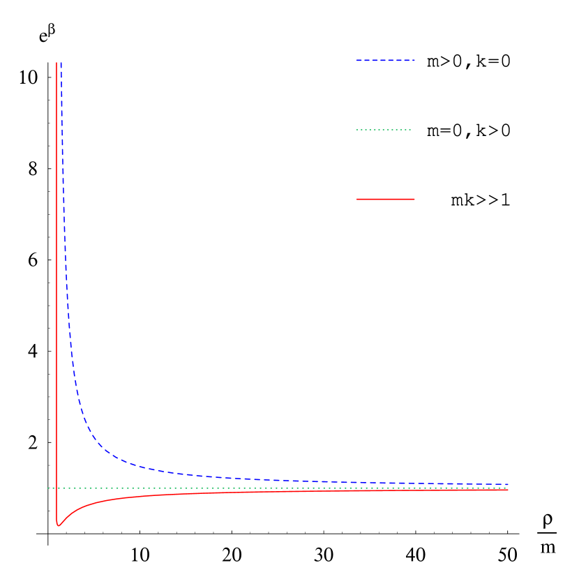
Figure 1: The function $e^{\beta}$ for different values of the pair (m,k).

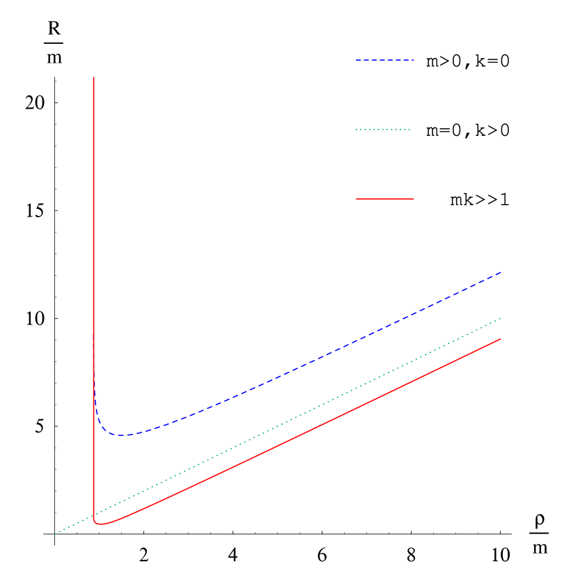
Figure 2: The function $\frac{\mathrm{R}}{\mathrm{m}}$ for different values of the pair (m,k).

To see what is going on, look at the standard radial coordinate $R(\rho)=\rho e^{\beta/2}$ depicted in figure 2 for different values of the pair $(m,k)$. The case $mk\gg 1$ we are treating here is similar to the case $(m>0,k=0)$ of equation (13) already discussed in [17] and will bring to analogous conclusions. More in detail, consider the proper circumference of radius $\rho$ given by $C(\rho)=2\pi R(\rho)$. We have that $C(\rho)$ becomes infinitely large as $\rho\to\infty$ and asymptotically very large, mantaining however finite, as $\rho\to\rho_{min}$ and has a minimum at $\rho_{0}\approx 1.04\,m$. This numerical value was estimated plotting the derivative $dR/d\rho$ versus $\rho$ and looking at the value of $\rho$ where it vanishes. The regions $\rho\in(\rho_{min},\rho_{0})$ and $\rho\in(\rho_{0},\infty)$ are two spacetimes associated with a wormhole whose throat occurs at $\rho_{0}$ where $C(\rho)$ is minimum. The wormhole is in this case aymmetric under the interchange of the asymptotic surfaces ($\rho=\rho_{min}$ and $\rho=\infty$) and traversable in principle due to the absence of event horizons. We verified numerically that the Kretchmann invariant becomes infinity only at $\rho=\sqrt{3}/2\,m$ which is not part of the manifold.

IV Conclusion

Some remarks seem here to be appropriate. First, it is known that a wormhole geometry can appear only if some of the energy conditions are violated and this requires the presence of some amount of “exotic” matter. The violation could be justified incorporating the cosmological constant into an energy-momentum tensor describing the vacuum contribution to the density and pressure. However wormhole solutions can be obtained also with vanishing cosmological constant in a Ricci flat spacetime, where energy conditions are trivially satisfied, of dimension $N\geq 5$ as in [17] where it was shown that every time an extra dimension is reduced a massless scalar field appears and plays the role of “exotic” matter. Also we would like to stress that in the framework of induced matter theory [19] the four-dimensional Einstein equations with sources can be locally embedded in five-dimensional Einstein equations without sources so although the matter seems exotic in four dimensions the five-dimensional spacetime on both sides of the throat is that of a vacuum and energy conditions are again trivially satisfied. Second, according to the common assumption made both in brane world and in induced matter theories, our five-dimensional metric tensor depends explicitly on the fifth coordinate, as can best seen inverting transformation (5) and applying it to the line element (7). One obtains

$$ds^{2}=\,e^{-2k|y|}\,\Big{\{}\Big{[}e^{\overline{\alpha}}+\dfrac{e^{\overline{\gamma}}k^{2}r^{2}e^{-2k|y|}}{(1+k^{2}r^{2}e^{-2k|y|})^{2}}\Big{]}dr^{2}+e^{\overline{\beta}}r^{2}d\Omega^{2}-\dfrac{e^{\overline{\gamma}}}{(1+k^{2}r^{2}e^{-2k|y|})}dt^{2}\Big{\}}$$

$$+\Big{[}e^{\overline{\alpha}}k^{2}r^{2}e^{-2k|y|}+\dfrac{e^{\overline{\gamma}}}{(1+k^{2}r^{2}e^{-2k|y|})^{2}}\Big{]}dy^{2}+2kre^{-2k|y|}\Big{[}-e^{\overline{\alpha}}+\dfrac{e^{\overline{\gamma}}}{(1+k^{2}r^{2}e^{-2k|y|})^{2}}\Big{]}drdy$$ (17)

where $\overline{\alpha}$, $\overline{\beta}$ and $\overline{\gamma}$ denote the functions $\alpha$, $\beta$ and $\gamma$ written in the coordinates $r$ and $y$. In this short letter we have not considered more general gauge transformations. Further investigations should have to take into account, as pointed out in [20], the influence that coordinate transformations may have on the interpretation of physical quantities in one lower dimension when in the reduced dimension is still present the extra coordinate.

References

- (1) N. Arkani-Hamed, S. Dimopoulos, G. Dvali, Phys. Lett. B 429 (1998) 263 hep-ph/9803315; Phys. Rev. D 59 (1999) 086004 hep-ph/9807344; I. Antoniadis, N. Arkani-Hamed, S. Dimopoulos, G. Dvali, Phys. Lett. B 436 (1998) 257 hep-ph/9804398.
- (2) L. Randall, R. Sundrum, Phys. Rev. Lett. 83 (1999) 3370 hep-ph/9905221.
- (3) L. Randall, R. Sundrum, Phys. Rev. Lett. 83 (1999) 4690 hep-th/9906064.
- (4) G. Dvali, G. Gabadadze, M. Porrati, Phys. Lett. B 485 (2000) 208 hep-th/0005016.
- (5) M. S. Morris, K. S. Thorne, Am. J. Phys. 56 (1988) 395; M. S. Morris, K. S. Thorne, U. Yurtsever, Phys. Rev. Lett. 61 (1988) 1449.
- (6) M. Visser, “Lorentzian Wormholes: from Einstein to Hawking”(AIP, Woodbury, 1995).
- (7) K. A. Bronnikov, Sung-Won Kim, Phys. Rev. D67 (2003) 064027, gr-qc/0212112.
- (8) S. Giddings, E. Katz, L. Randall, JHEP 0003 (2000) 023 hep-th/0002091.
- (9) I. Giannakis, H. C. Ren, Phys. Rev. D63 (2001) 024001 hep-th/0007053.
- (10) H. Kudoh, T. Tanaka, Phys. Rev. D64 (2001) 084022 hep-th/0104049.
- (11) G. C. McVittie, Mon. Not. R. Astron. Soc. 933 (1933) 325.
- (12) L. K. Patel, R. Tikekar, N. Dadhich, Grav. Cosmol. 6 (2000) 335 gr-qc/9909069.
- (13) H. P. Robertson, Phil. Mag. 5 (1928) 835.
- (14) A. Davidson, D. A. Owen, Phys. Lett. B 155 (1985) 247.
- (15) P. S. Wesson, Phys. Lett. B 276 (1992) 299.
- (16) D. J. Gross, M. J. Perry, Nucl. Phys. B 226 (1993) 29.
- (17) A. G. Agnese, M. La Camera, Phys. Rev. D 58 (1998) 087504 gr-qc/9806074.
- (18) R. Maartens, Prog. Theor. Phys. Suppl. 148 (2002) 213, gr-qc/0304089.
- (19) P. A. Wesson, “Space-Time-Matter” (World Scientific, Singapore, 1999).
- (20) J. Ponce de Leon, Int J. Mod. Phys. D 11 (2002) 1355 gr-qc/0105120.