Electromagnetic Generators and Detectors of Gravitational Waves

Abstract

The renewed serious interest to possible practical applications of gravitational waves is encouraging. Building on previous work, I am arguing that the strong variable electromagnetic fields are appropriate systems for the generation and detection of high-frequency gravitational waves (HFGW). The advantages of electromagnetic systems are clearly seen in the proposed complete laboratory experiment, where one has to ensure the efficiency of, both, the process of generation and the process of detection of HFGW. Within the family of electromagnetic systems, one still has a great variety of possible geometrical configurations, classical and quantum states of the electromagnetic field, detection strategies, etc. According to evaluations performed 30 years ago, the gap between the HFGW laboratory signal and its level of detectability is at least 4 orders of magnitude. Hopefully, new technologies of today can remove this gap and can make the laboratory experiment feasible. The laboratory experiment is bound to be expensive, but one should remember that a part of the cost is likely to be reimbursed from the Nobel prize money ! Electromagnetic systems seem also appropriate for the detection of high-frequency end of the spectrum of relic gravitational waves. Although the current effort to observe the stochastic background of relic gravitational waves is focused on the opposite, very low-frequency, end of the spectrum, it would be extremely valuable for fundamental science to detect, or put sensible upper limits on, the high-frequency relic gravitational waves. I will briefly discuss the origin of relic gravitational waves, the expected level of their high-frequency signal, and the existing estimates of its detectability.

I Introduction

The engineers and enterpreneures are rightly seeing in gravitational waves (g.w.) a new opportunity, even though, at this moment of time, this opportunity does not look like having a chance of becoming practical in foreseeable future. However, we have many examples of wrong prognoses. It is known that when the discoverer of the nucleus, Lord Rutherford, was asked about the possible practical applications of nuclear energy, he answered “never”. It is very likely that the gravitational radiation will eventually become useful, say, for purposes of communication. But in any case, it is difficult to imagine that we will go along without attempting to demonstrate in laboratory conditions the possibility of controllable generation and detection of gravitational waves. The laboratory experiment is a necessary first step to possible practical applications of g.w., and it is this first step that will be mostly discussed in this contribution.

Gravitational waves are less mysterious than one can gather from popular accounts. The relativistic Einstein’s gravity is usually described in geometrical terms, as curvature of space-time. Correspondingly, gravitational waves are often described as “oscillations of space-time itself”. This characterisation is quite puzzling and distressing for a practically-minded person. It makes defunct the usual physical intuition based on electromagnetic waves and other propagating physical fields. It makes one to suspect that there may be something artificial and unreal in the “waves of space-time itself”. But this characterisation is only a matter of unfortunate language. Geometrical concepts are useful for some purposes, but they are greatly misleading for others. One should remember that although the Einstein gravity can be described in geometrical terms, it is also a normal physical field. The gravitational field is universal in all its interactions with itself and other fields and matter, and this is what makes the geometrical formulation of relativistic gravity possible, but the geometrical formulation is not necessary and is not obligatory. In fact, it would be a nightmare to try to discuss the laboratory gravitational-wave experiment in terms of differential geometry and “oscillating space-time”, rather than in the engineering terms of the emitted and absorbed physical radiation.

The relativistic gravitational field is governed by the non-linear wave equations - the Einstein equations. However, in many situations one can neglect the non-linearities of the gravitational field. In particular, very often one can neglect the interaction of gravitational waves with other gravitational fields and with themselves. In this case, we come to the notion of linearized gravity and weak gravitational waves. Certainly, in any laboratory experiment we will be dealing with extremely weak gravitational waves. Weak g.w. are very far from being mysterious; they may even appear quite boring and disappointing. Indeed, there is not so much difference with electromagnetic waves in terms of their general properties, but gravitational waves interact with matter and other fields much-much less effectively than electromagnetic waves. Gravitational waves carry their energy practically without scattering and absorption. This is why it is so difficult to detect astronomical gravitational waves. But the other side of this difficulty is the tremendous penetrating capability of gravitational waves. This is why they are so important as a tool of astronomical research, and this is why they attract attention as a possible unique means of communication.

The relativistic gravitational field can be described by 10 components of the $4\times 4$ symmetric dimensionless tensor $h^{\mu\nu}$. The components of $h^{\mu\nu}$ are functions of time and spatial coordinates $x^{\alpha}=(ct,x,y,z)$. The functions $h^{\mu\nu}$ obey the nonlinear wave-like dynamical equations - the Einstein equations. The energy-momentum tensor $t^{\mu\nu}$ of the gravitational field is calculable from the field tensor $h^{\mu\nu}$.

The linearised gravitational waves satisfy the wave equation

$${h^{\mu\nu,\alpha}}_{,\alpha}+\eta^{\mu\nu}{h^{\alpha\beta}}_{,\alpha,\beta}-{h^{\nu\alpha,\mu}}_{,\alpha}-{h^{\mu\alpha,\nu}}_{,\alpha}=0,$$ (1)

where the ordinary derivative is denoted by a comma and $\eta^{\mu\nu}$ is the metric tensor of the Minkowski space-time:

$${\rm d}\sigma^{2}=\eta_{\mu\nu}{\rm d}x^{\mu}{\rm d}x^{\nu}=c^{2}{\rm d}t^{2}-{\rm d}x^{2}-{\rm d}y^{2}-{\rm d}z^{2}.$$ (2)

The first term in Eq. (1) is the familiar d’Alembert (wave) operator:

$\displaystyle{h^{\mu\nu,\alpha}}_{,\alpha}=\left(\frac{\partial^{2}}{c^{2}\partial t^{2}}-\frac{\partial^{2}}{\partial x^{2}}-\frac{\partial^{2}}{\partial y^{2}}-\frac{\partial^{2}}{\partial z^{2}}\right)h^{\mu\nu}.$

A plane-wave solution to Eq. (1) is given by

$$h^{\mu\nu}=a^{\mu\nu}e^{ik_{\alpha}x^{\alpha}}+{\it c.c.},$$ (3)

where $k_{\alpha}k^{\alpha}=0$, reflecting the fact that a g.w. propagates with the speed of light. Because of this condition, the field equations (1) require the 10 components of the constant matrix $a^{\mu\nu}$ to satisfy 4 constraints: $a^{\mu\nu}k_{\nu}=0$. Among the remaining 6 components, only 2 degrees of freedom (sometimes called the TT-components $\tilde{a}^{ij}$) are physically important, in the sense that it is only these degrees of freedom that fully determine the observational manifestations of the plane wave and its energy-momentum characteristics. Indeed, it is easy to show that the gravitational energy-momentum tensor

$$t_{\mu\nu}=\frac{c^{4}}{32\pi G}\left[{h^{\alpha\beta}}_{,\mu}h_{\alpha\beta,\nu}-\frac{1}{2}h_{,\mu}h_{,\nu}\right]$$ (4)

depends only on the TT-components of the field and its two independent amplitudes $h_{+}$ and $h_{\times}$:

$$t_{\mu\nu}=\frac{c^{4}}{32\pi G}k_{\mu}k_{\nu}\left[2\tilde{a}^{ij}\tilde{a}^{*}_{ij}\right]=\frac{c^{4}}{32\pi G}k_{\mu}k_{\nu}\left[h_{+}^{2}+h_{\times}^{2}\right].$$ (5)

In this expression we have dropped (as we normally do in the case of energy-momentum tensor for the electromagnetic waves) the purely oscillatory terms.

The amplitudes $h_{+},h_{\times}$ are determined by the source of the gravitational waves. To find the amplitudes, we should replace the zero in the right hand side of Eq. (1) by the source term $(16\pi G/c^{4})T^{\mu\nu}$, where $T^{\mu\nu}$ is the energy-momentum tensor of the source, and seek the retarded solutions to the inhomogeneous wave equation. For example, for a pair of stars in a circular orbit, with masses of the stars $M_{1}$, $M_{2}$, located at the distance $R_{0}$ from us, and after averaging over the orbital period and orientation of the orbital plane, we obtain

$$h=\left(\langle h_{+}^{2}\rangle+\langle h_{\times}^{2}\rangle\right)^{1/2}=\left(\frac{32}{5}\right)^{1/2}\frac{1}{R_{0}}\frac{G^{5/3}}{c^{4}}\frac{M_{1}M_{2}}{(M_{1}+M_{2})^{1/3}}(\pi f)^{2/3},$$ (6)

where the emitted g.w. frequency $f$ (in $Hz$) is twice the orbital frequency.

Roughly, the characteristic amplitude $h$ from a given source is given by

$$h_{ij}\approx\frac{G}{c^{4}}\int\frac{T_{ij}(t_{ret})}{r}dV~{}~{}~{}~{}~{}{\rm and}~{}~{}~{}~{}~{}h\approx\frac{1}{R_{0}}\frac{GM}{c^{2}}\left(\frac{v}{c}\right)^{2},$$ (7)

where $M$ is the total mass of the source and $v$ is the characteristic velocity of the matter bulk motion. This formula is quite universal, and it can also be written in terms of the characteristic variable stresses $\sigma$ within the source, and the source’s volume $V$:

$$h\approx\frac{1}{R_{0}}\frac{G}{c^{4}}\sigma V.$$ (8)

As long as the retardation effects inside the source can be neglected, this formula is equally well applicable to the radiating systems of any nature - in cosmos and in laboratory, mechanical and electromagnetic.

II Current status of the astronomical program and its comparison with a HFGW laboratory program

The dimensionless number $h$ is a very convenient characterisation of the strenght of a given g.w. and its detectability. Under the action of a gravitational wave, a pair of free masses, initially separated by the distance $l$, experience relative oscillatory displacements proportional to the incoming wave amplitude $h$: $\delta l/l\approx h$. Very powerful astronomical sources, currently under intense experimental g.w. searches [1], [2], [3], produce something like $h\approx 10^{-22}$ at Earth. This is an increadibly small number. It enters any conceivable method of detection of gravitational waves and explains why it is so difficult to observe them. For example, in a $4km$-long laser interferometer, such as LIGO, we need to beat all the noises and measure the mirror’s displacements at the level of $4\times 10^{-17}cm$. At the same time, the flux of energy $F=ct^{0i}$ at Earth from the discussed sources is quite impressive by astronomical standards. At the representative frequency $f=200Hz$, the flux reaches $F\approx 3\times 10^{-2}erg/sec~{}cm^{2}$. But most of this energy passes through the g.w. detectors without scattering and absorption. This is why, in the gravitational-wave physics, such characteristics as watts and joules may be misleading. The dimensionless amplitude $h$ is more adequate. But in any case, whatever the units in which the analysis is being carried out, only a joint discussion of the complete system (emitter plus detector) gives the correct evaluation of what is “small” or “big”, easy to detect or extremely difficult to detect.

The recently assembled LIGO interferometers are approaching their planned level of sensitivity. It appears that, at the time of writing, there still exists a gap in one order of magnitude, in terms of $h$, between the actually reached level of sensisitivity and the design sensitivity [1]. One should clearly understand what is likely to happen when the design level of sensitivity of the initial interferometers is finally achieved. Baring the extremely fortunate surprises, we will probably be able to see only the most powerful, but rare, sources, such as coalescing binary stellar-mass black holes. Less powerful, even if more numerous, sources - coalescing binary neutron stars, are unlikely to be seen, because the expected signal-to-noise ratio is somewhat smaller than 1. For a guaranteed detection of astronomical sources, the experimenters will have to improve the sensitivity by one further order of magnitude, as compared with the design sensitivity of the initial instruments. This is the goal of the so-called advanced interferometers, and this goal will probably be reached by 2007. (For more details on the current status of the gravitational wave astronomy see, for example, [2], [3].)

There is little doubt that the astronomical program will completely dominate, and rightly so, any other experimental efforts in the gravitational-wave physics for some time to come. Having said that, one can still wonder whether a laboratory experiment is much more difficult to realise than to build equipment for the observation of cosmic gravitational waves. Of course, the justifications for these efforts are totally different. In gravitational-wave astronomy we directly explore the fascinating Universe, whereas in the laboratory experiment we are likely to confirm a theory (true, very fundamental theory, but anyway tested also by other means), with very remote prospects for practical applications of gravitational radiation. However, the justification for the laboratory experiment is sufficiently convincing. A more difficult question is its feasibility. Here, one will have to admit that the both enterprises are very difficult. Surprisingly, the laboratory program does not appear to be unacceptably more difficult than the cosmic program. If we take as a benchmark the 4 orders of magnitude separating the detecting and generating capabilities in laboratory (see Sec. IV below), it is like having 1 dollar instead of required 10000. But, strictly speaking, in the cosmic program we also have, at the time of writing, only something like 1 dollar instead of required 100 (see above). The difference between the two programs is substantial, but not ridiculously large.

As an additional motivation for the experimental work on HFGW, there are arguments showing that it can be complementary and useful for the astronomical program. First, there exists the fundamentally important cosmological signal - relic gravitational waves. The high-frequency end of the spectrum is the most natural interval for the high-frequency techniques, and first of all for electromagnetic detectors (see Sec V below). Second, part of the high-frequency studies with electromagnetic detectors may eventually be useful for laser interferometers of the next generation. Indeed, it is quite likely that in order to reach the required level of sensitivity we will be forced to implement the sophisticated techniques such as squeezed light and quantum-nondemolition measurements (see, for example, [4]) and this is where the expertise of the HFGW community can be useful.

III Efficiency of gravitational-wave emitters

Astronomical sources are immensely more powerful than any conceivable sources at Earth, but they are very far away from us, and not under our control. In contrast, in laboratory, one can place the emitter and the detector very close to each other, choose the appropriate materials, implement the coherence and focusing of the emitted radiation, use the advantages of the resonant detection, etc. One usually illustrates the hopelessness of laboratory g.w. experiments by giving an example of the meager gravitational radiation generated by a rotating massive rod. Well, if you are so naive that you plan to rotate a rod, then the enterprise may indeed be hopeless. But surely there must exist something smarter. Let us give a general comparative analysis of possible mechanical and electromagnetic systems [5].

Let us consider an elementary mechanical emitter ($m$-emitter) and an elementary electromagnetic emitter ($e$-emitter). By the elementary we mean a source that occupies a volume of order $\lambda_{s}^{3}$ in the first case and $\lambda_{e}^{3}$ in the second case; $\lambda_{s}$ and $\lambda_{e}$ are the wavelengths of the acoustic and electromagnetic waves. A vibrating object and an oscillating electromagnetic wave in a cavity are examples of $m-$ and $e-$ emitters respectively. For the comparison to be fair, the sources are assumed to emit g.w. with one and the same wavelength $\lambda_{g}$ and are placed at the same distance $R_{0}$ from the observer.

Let $A$ be the amplitude of elastic vibrations in the $m$-emitter. Then the characteristic amplitude of the stress tensor $T_{ij}$ is $\sigma_{m}\approx\rho_{m}v_{s}^{2}(A/\lambda_{s})$, where $\rho_{m}$ is the density of the material and $v_{s}^{2}$ is the square of the sound speed. Since $\nu_{g}=c/\lambda_{g}\approx v_{s}/\lambda_{s}$, we have $\lambda_{s}\approx(v_{s}/c)\lambda_{g}\ll\lambda_{g}$ which means that the body of the elementary $m$-emitter is situated deeply inside the inductive zone of the gravitational radiation and, hence, the retardation effects within the source are negligibly small. For the g.w. amplitude we obtain from Eq. (8):

$$h_{m}\approx\frac{G}{c^{4}}\frac{1}{R_{0}}\sigma_{m}\lambda_{s}^{3}.$$ (9)

Let us now consider an elementary $e$-emitter. The amplitude $\sigma_{e}$ of the electromagnetic stress has the order of magnitude of the energy density ${\epsilon}_{e}$ of the varying electromagnetic field, $\rho_{e}c^{2}={\epsilon}_{e}$, i.e. $\sigma_{e}\approx{\epsilon}_{e}$. Since $\nu_{g}=c/\lambda_{g}\approx c/\lambda_{e}$, the volume of the elementary $e$-emitter is of the order of $\lambda_{g}^{3}$, that is, it is still at the limit of applicability of Eq. (8) with the retardation effects ignored. The amplitude of the emitted gravitational wave is

$$h_{e}\approx\frac{G}{c^{4}}\frac{1}{R_{0}}\sigma_{e}\lambda_{g}^{3}.$$ (10)

The ratio of (9) and (10) is

$$\frac{h_{m}}{h_{e}}\approx\frac{\rho_{m}}{\rho_{e}}\left(\frac{v_{s}}{c}\right)^{5}\frac{A}{\lambda_{s}}.$$ (11)

Using the reasonable parameters: $\rho_{m}\approx 1g/cm^{3},~{}\rho_{e}\approx 10^{-18}g/cm^{3},~{}v_{s}/c\approx 10^{-5},~{}A/\lambda_{s}\approx 10^{-3}$, we find that $h_{m}/h_{e}\approx 10^{-10}$. In other words, an elementary $e$-emitter is much more efficient than an elementary $m$-emitter. However, the comparison is not entirely fair as the volume of the former, $\lambda_{g}^{3}$, is much larger than the volume of the later, $\lambda_{s}^{3}$. In the volume of an elementary $e$-emitter one can accomodate a large number $N=(\lambda_{g}/\lambda_{s})^{3}\approx(c/v_{s})^{3}\gg 1$ of elementary $m$-emitters. Under the condition that they all are phased to work coherently, the total g.w. amplitude is the sum of individual amplitudes, and it can be as large as $h_{mc}\approx Nh_{m}$. Then, we finally obtain

$$\frac{h_{mc}}{h_{e}}\approx\frac{\sigma_{m}}{\sigma_{e}}.$$ (12)

This formula answers all the principal questions. We see that the most important parameter is the maximal reachable amplitude of the dynamical stresses. Extremely high stresses, at the limit of static breaking point, for very strong materials, is in the range of $\sigma_{m}\approx 10^{9}dyne~{}cm^{2}$. Similar variable stresses can be obtained by producing and maintaining variable electromagnetic fields with characteristic field strength $E\approx H\approx 10^{5}gauss$. Then, an elementary $e$-emitter, having the volume $\lambda_{g}^{3}\approx 10^{6}cm^{3}$, produces a g.w. amplitude $h\approx 10^{-36}$ at the boundary of the wave zone, and emits the total power $W\approx 4\times 10^{-13}erg/sec$. To raise the amplitude and power, one would have to implement large composite systems.

This analysis illustrates the advantages of the electromagnetic systems. First, the coherence of the source is automatically achieved in a large volume $\sim\lambda_{g}^{3}$. The huge number of mechanical emitters placed in the same volume would need to be specially phased in order to achieve the constructive interference of the emitted gravitational radiation. Second, it seems that it is much easier to manufacture a simple electromagnetic emitter (essentially, an oscillating eigen-mode of the electromagnetic field in a cavity) than try to pack together a large number of specially phased mechanical emitters. Third, the efficient generation process suggests the similar (inverse) process of detection. It seems natural to use the electromagnetic systems also as the detection technique.

IV Complete laboratory experiment

The important concern for the succcess of the laboratory experiment is to ensure the focusing, as much as possible, of the emitted g.w. power in one place, rather than to let it be dispersed over all directions. This was one of motivations for the specific geometrical configuration suggested in [6]. It is proposed that the emitter is a torus-like electromagnetic resonator with a rectangular cross-section (see Fig. 1). The oscillating electromagnetic field in the resonator produces a standing gravitational wave in the focal region, near the axis of symmetry. The gravitational wave is standing because the emitted cylindrical gravitational wave passes through the axis of symmetry and interferes with itself. The gravitational-wave frequency $\Omega$ is twice the frequency of the variable electromagnetic field in the generator, $\Omega=2\omega$. Another resonator is placed in the focal region and plays the role of the detector. Its resonant frequency is tuned to the frequency of the gravitational wave $\Omega$. Among the advantages of this particular configuration is its geometrical simplicity, which allows one to find exact solutions to the Maxwell equations, both, in the generator and in the detector.

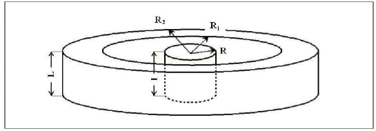
FIG. 1.: Scheme of a possible laboratory experiment

Although almost all the calculations [6] have been performed exactly, it is convenient to use the order of magnitude evaluations which follow from the calculations, and which, of course, coincide with the evaluations outlined above. The very important estimate, which we did not discuss yet, is the detectabilty condition.

The analysis shows that the change of energy $\Delta{\cal E}$ in the resonator-detector depends on whether the initial electromagnetic field in the detector is realised as a constant (say, magnetic) field, or as a an oscillating resonant electromagnetic eigen-mode. It is assumed that the accumulation of the signal is taking place during the relaxation time $\tau^{*}=Q/\Omega$, where $Q$ is the quality factor of the resonator-detector. Then, in the first case, $\Delta{\cal E}\approx(hQ)^{2}{\cal E}$, where ${\cal E}=(H^{2}/8\pi)V$. And in the second case, $\Delta{\cal E}\approx(hQ){\cal E}$, where ${\cal E}=(E^{2}/4\pi)V$. These formulas show that the responses of the detector are different in these two options. But the natural electromagnetic noises are also different. One should impose different criteria in order to determine whether the one and the same g.w. signal is detectable or not. In the first case, one can think that one can distinguish one “photon” (a resonant mode exitation with energy ${\cal E}\sim\hbar\Omega$) on the background of a constant (magnetic) field. In the second case, one should typically assume that only the number $\sqrt{N}$ of new “photons” can be distinguished on the background of the already existing $N$ “photons”, $N={\cal E}/\hbar\Omega$. Combining each of responses with the corresponding detectability condition, one finds that there is in fact no much difference between these two cases in terms of the measurable amplitude $h$. The order of magnitude evaluation shows that the detectable $h$ is

$$h_{det}\approx\sqrt{\frac{\hbar\Omega}{{\cal E}}}\frac{1}{Q}.$$ (13)

The situation can, however, change considerably in favor of the second option, if one succeeds in realising a special (quantum) state of the electromagnetic field in the detector, such that the variance of the number of quanta $N$ is much smaller than $\sqrt{N}$. Then, assuming that the quantum non-demolition measurement can distinguish the energy of, say, a few new quanta on the backgound of a huge (mean) number of quanta in the detector, the detectable g.w. amplitude $h_{det}$ can be significantly lowered. We will first continue our estimates without taking this possibility into account, but will return to it later.

The geometry of the system allows one to choose the following optimal parameters: $L\approx l\approx\lambda$, where $\lambda=2\pi c/\Omega$, $R\approx 2\lambda/3,~{}R_{1}\approx 2\lambda,~{}R_{2}\approx 7\lambda/2$. Then the detectability condition can be written as

$$\lambda^{4}E^{2}HQ\approx 30\frac{c^{4}}{G}\sqrt{\hbar c},$$ (14)

where $E$ is the amplitude of the oscillating field in the generator and $H$ is the typical (possibly, constant magnetic) field in the detector. Let us take for illustration $\lambda\approx 10^{2}cm,~{}E\approx H\approx 3\times 10^{5}gauss,~{}Q\approx 7\times 10^{13}$. Then, the left-hand side of Eq. (14) is 4 orders of magnitude smaller than the right-hand side of the same formula. It is this gap of 4 orders of magnitude that we referred to in the Abstract.

One possibility to satisfy Eq. (14) is to simply increase the size of the system, going from $\lambda\approx 10^{2}cm$ to $\lambda\approx 10^{3}cm$. Another possibility would be to raise the product $E^{2}HQ$ by the same 4 orders of magnitude. Probably the most elegant and realistic possibility is to try and improve the detectability condition by using the sophisticated quantum states of the electromagnetic field in the detector, that we mentioned earlier. Certainly, the laboratory experiment is going to be difficult, but it seems worth of trying.

V Electromagnetic detectors for relic gravitational waves

In laboratory conditions, and in almost all astrophysical situations, one can completely neglect the non-linearities of gravity, that is, the interaction of gravitational waves with other gravitational fields. However, this is not always the case. The most important example is the interaction of gravitational waves with the strong variable gravitational field of the very early Universe. One can use the engineering intuition in order to understand what is going on here. A gravitational wave can be thought of as a harmonic oscillator, while the smooth variable gravitational field of the surrounding Universe as a gravitational pump field. The g.w. oscillator is parametrically coupled to the gravitational pump field. This specific coupling follows from the non-linear structure of the Einstein equations. This coupling provides a mechanism for the superadiabatic (parametric) amplification of classical waves and for the quantum-mechanical generation of waves from their zero-point quantum oscillations [3]. The word “superadiabatic” emphasizes the fact that this effect takes place over and above whetever happens to the wave during very slow (adiabatic) changes of the pump field. That is, we are interested in the increase of occupation numbers, rather than in the gradual shift of energy levels. The word “parametric” emphasizes the mathematical structure of the wave equation. A parameter of the oscillator, namely its frequency, is being changed by the variable pump field. It is this sufficiently rapid change of frequency of the oscillator that is responsible for the considerable increase of energy of that oscillator.

The parametric amplification of the inevitable zero-point quantum oscillations leads to the generation of a stochastic background of relic gravitational waves. The mechanism itself is based on the fundamental physics only, but the generated signal depends on the pump field. In other words, the amount of relic gravitational waves depend on a concrete cosmological model of the very early Universe. Combining the theory with the available cosmological data, one can evaluate the expected level of high-frequency relic gravitational waves [3]. For example, the root-mean-square (r.m.s.) amplitude is expected to reach $h_{r.m.s.}\approx 10^{-30}$ at $\nu=10^{7}Hz$. The amplitude is smaller at higher frequencies. It may reach $h_{r.m.s.}\approx 10^{-32}$ at $\nu=10^{11}Hz$, but then it should quickly decrease as a function of higher frequencies. There is no much sense to expect any relic gravitational waves at frequencies higher than that.

We may be lucky (although it does not seem very likely) if the thermal background of gravitational waves survived until now. Then, in the vicinity of $\nu=10^{11}Hz$ there will be a maximum of the Planck spectrum. The amplitude of the Planck spectrum can be in the region of $h_{r.m.s.}\approx 3\times 10^{-32}$, but not very much larger than this. The quoted numbers for relic and thermal backgrounds give the feeling of what we can expect of high-frequency cosmic gravitational waves.

What can be said about the detectability of relic gravitational waves ? The first impression is that they may be easier to detect than the gravitational waves produced in laboratory. For example, at $\nu=10^{7}Hz$, the amplitude of relic gravitational waves, $h_{r.m.s.}\approx 10^{-30}$, is several orders of magnitude higher than the realistic amplitude of laboratory gravitational waves (see Sec. IV). Unfortunately, this does not mean that the relic gravitational waves are easier to detect. The crucial difference is in the character of these two signals. The laboratory signal is essentially a deterministic monochromatic wave, which allows one to systematically accumulate the response amplitude. In contrast, relic gravitational waves form a random signal, which allows only an accumulation of energy. When it comes to evaluation of the detectable amplitude of relic gravitational waves [7], formula (13) should be modified. Under the same conditions that formula (13) was derived, but now for the stochastic signal, we obtain

$$h_{det}\approx\sqrt{\frac{\hbar\Omega}{{\cal E}}}\frac{1}{\sqrt{Q}}.$$ (15)

Applying this formula to a simple electromagnetic detector, we can expect to measure $h_{det}\approx 10^{-26}$ instead of the required level of the cosmic signal $h_{r.m.s.}\approx 10^{-30}$.

This gap is sufficiently wide to discount hopes to bridge this gap by longer observation time, or cross-correlation of several detectors, etc. It appears that the sensitivity of electromagnetic detectors can reach the required level only if the squeezed quantum states of the electromagnetic field in the detector, and quantum non-demolition measurements, are implemented. Aternatively, one can think of large composite systems (“large crystal” [7]), where the individual elements are arranged to work more coherently than simply absorbing gravitational radiation independently one from other. Although these techniques seem possible in principle, so far, there is no concrete proposals how to implement them in practice. Regrettably, the detection of high-frequency relic gravitational waves will probably be even more challenging problem than their detection in low-frequency and very low-frequency bands. Smart ideas are badly needed.

REFERENCES

- [1] http://www.ligo.caltech.edu
- [2] C. Cutler and K. S. Thorne. In: General Relativity and Gravitation, Eds. N.T.Bishop and S.D.Maharaj, (World Scientific, 2002) p. 72
- [3] L. P. Grishchuk. Update on gravitational-wave research, ArXive: gr-qc/0305051
- [4] V. B. Braginsky, M. L. Gorodetsky, F. Ya. Khalili, A. B. Matsko, K. S. Thorne, and S. P. Vyatchanin. ArXive: gr-qc/0109003
- [5] L. P. Grishchuk. Phys. Lett. 56A, 255 (1976)
- [6] L. P. Grishchuk and M. V. Sazhin. Zh. Eksp. Teor. Fiz. 68, 1569 (1975) [Sov. Phys. JETP. 41, 787 (1976)]; L. P. Grishchuk. Usp. Fiz. Nauk. 121, 629 (1977) [Sov. Phys. Usp. 20, 319 (1977)]
- [7] L. P. Grishchuk. Pis’ma Zh. Eks. Teor. Fiz. 23, 326 (1976) [JETP Lett. 23, 293 (1976)]; Usp. Fiz. Nauk. 156, 297 (1988) [Sov. Phys. Usp. 31, 940 (1989)]