Gyromagnetic ratio of rapidly rotating compact stars in general relativity

Abstract

We numerically calculate equilibrium configurations of uniformly rotating and charged neutron stars, in the case of insulating material and neglecting the electromagnetic forces acting on the equilibrium of the fluid. This allows us to study the behaviour of the gyromagnetic ratio for those objects, when varying rotation rate and equation of state for the matter. Under the assumption of low charge and incompressible fluid, we find that the gyromagnetic ratio is directly proportional to the compaction parameter $M/R$ of the star, and very little dependent on its angular velocity. Nevertheless, it seems impossible to have $g=2$ for these models with low charge-to-mass ratio, where matter consists of a perfect fluid and where the collapse limit is never reached.

1 Introduction

For steadily rotating, charged massive bodies, the gyromagnetic factor $g$ is defined as the ratio

$$g=\frac{2M{\cal M}}{QJ};$$ (1)

where $M$ is the mass, $Q$ the total charge and $J$ the angular momentum of the system. $\cal M$ is the magnetic moment of the system, linked with the motion of the charges that are accounting for $Q$. With such a definition, in classical electrodynamics a rotating charged particle has a gyromagnetic factor equal to 1. The same is thus true for any system in classical electrodynamics, with a constant ratio of charge and mass density. On the other hand, within general relativity, the gyromagnetic ratio for all charged and rotating black holes is $g=2$. Many points concerning the gyromagnetic ratio for isolated systems within classical electrodynamics, quantum theory and general relativity have been studied by Pfister and King [1]. The question we try to address here is the following one. How does the gyromagnetic factor behave for “intermediate” objects in general relativity, that possess a gravitational field weaker than that of black holes, but in which strong field effects are not negligible?

The aim of this paper is to try to answer this question by numerically studying the $g$-factor of rotating and charged relativistic compact stars, within the framework of general relativity. We use a self-consistent physical model, in which matter is supposed to be a charged (insulator type) perfect fluid; axisymmetric and in stationary rotation. As it will be shown later, the only limitation shall be on neglecting the electromagnetic forces acting on hydrodynamic equilibrium, making our study a “low charge” approximate one; but we take into account the electromagnetic field contribution to the total energy-momentum tensor. The variation of the gyromagnetic ratio as a function of the number of particles in the system, or as a function of the rotation frequency will also be discussed. Details of the physical model are presented in section 2, section 3 is then giving results of the numerical study for two equations of state, which determine local properties of matter, and making comparison with previous works. Finally, section 4 summarises results and gives some concluding remarks.

2 Model and assumptions

We here give the most important assumptions made in our study; complete details of the formalism and the way numerical stars are computed can be found in Bonazzola et al. [2] and in Bocquet et al. [3] for the magnetised configurations.

2.1 Stationary and axisymmetric spacetime

We want to solve the coupled Einstein-Maxwell equations to get general relativistic magnetised models of stationary rotating bodies. We make the assumption that the spacetime is also stationary (asymptotically timelike Killing vector field), axisymmetric (spacelike Killing vector field which vanishes on a timelike 2-surface, axis of symmetry and whose orbits are closed curves) and asymptotically flat. In addition, we suppose that the source of the gravitational field satisfies the circularity condition, equivalent to the absence of meridional convective currents and only poloidal magnetic field is allowed. We then use MSQI (Maximal Slicing - Quasi Isotropic, see [2]) coordinates $(t,r,\theta,\varphi)$, in which the metric tensor takes the form

$$\rmd s^{2}=g_{\mu\nu}\rmd x^{\mu}\rmd x^{\nu}=-N^{2}\rmd t^{2}+B^{2}r^{2}\sin^{2}\theta(\rmd\varphi-\beta^{\varphi}\rmd t)^{2}+A^{2}(\rmd r^{2}+r^{2}\rmd\theta^{2}),$$ (2)

where $N,\beta^{\varphi},A$ and $B$ are four functions of $(r,\theta)$.

With our hypothesis, the electromagnetic field tensor $F_{\alpha\beta}$ must be derived from a potential 1-form with the following components

$$A_{\alpha}=(A_{t},0,0,A_{\varphi}).$$ (3)

The Einstein-Maxwell equations result in a set of six coupled non-linear elliptic equations for the four metric and the two electromagnetic potentials (see [2] and [3]). The right-hand side of this system also involves matter terms (density and charge currents), which will be discussed in next section.

2.2 Fluid properties

The matter is supposed to consist of a perfect fluid, so there exists a privileged vector field: the 4-velocity $u^{\alpha}$. The energy-momentum tensor takes its usual form

$$T^{\mu\nu}=(e+p)u^{\mu}u^{\nu}+pg^{\mu\nu}+T^{\mu\nu}_{\rm EM},$$ (4)

where $p$ is the fluid pressure and $e$ the energy density measured in the fluid frame. $T^{\mu\nu}_{\rm EM}=1/(4\pi)\left(F^{\mu\alpha}F^{\nu}_{\alpha}-1/4F_{\alpha\beta}F^{\alpha\beta}g^{\mu\nu}\right)$ is the electromagnetic contribution to the energy-momentum tensor. Following [2], we note $\Omega=u^{\varphi}/u^{t}$ and define $\Gamma$ as the Lorentz factor linking the fluid comoving observer and the locally non-rotating one. We make the assumption that the matter is rigidly rotating ($\Omega=$constant) and that the equation of state (EOS) is a one parameter EOS (ignoring the influence of temperature): $e=e(n_{\rm B})$ and $p=p(n_{\rm B})$, with $n_{\rm B}$ being the proper baryon density.

The momentum-energy conservation gives an equation of stationary motion for the fluid, which can be written as a first integral of motion (the electromagnetic contribution to the energy-momentum tensor is not considered yet), see [2]

$$\ln\frac{e+p}{n_{\rm B}}+\ln N-\ln\Gamma=\rm{constant}.$$ (5)

We turn now to the electromagnetic part; in order to have a complete charged body, with a constant ratio of charge and mass density (see [1]), we suppose, contrary to [3] or [4], that our system consists of an insulator, so that currents originate only from macroscopic charge movement. The 4-current is thus proportional to $j^{\mu}\sim u^{\mu}/\Gamma$ implying that $j^{\varphi}=\Omega j^{t}$. Taking then electromagnetic force term $f_{i}=F_{i\sigma}j^{\sigma}/(e+p)$ into account, the momentum-energy conservation reads

$$\partial_{i}\left(\ln\frac{e+p}{n_{\rm B}}+\ln N-\ln\Gamma\right)+\frac{1}{e+p}j^{t}\partial_{i}\left(\Omega A_{\varphi}-A_{t}\right)=0.$$ (6)

The integrability condition of this equation is that the last term is a gradient, so that there exists a function $M(r,\theta)$ such that $j^{t}\partial_{i}\left(\Omega A_{\varphi}-A_{t}\right)=(e+p)\partial_{i}M$. Following the same arguments as in [2], there must exist a regular function $m$, such that

$$j^{t}=(e+p)m\left(\Omega A_{\varphi}-A_{t}\right),\quad{\rm with}\quad M(r,\theta)=\int_{0}^{\Omega A_{\varphi}(r,\theta)-A_{t}(r,\theta)}m(x)\rmd x.$$ (7)

But, this gives too large a freedom for the distribution of charged particles inside the star. In particular, the charge density $j^{t}$ is independent of the baryon density $n_{\rm B}$, and the $g$-factor can, in principle, take any value. It is also irrelevant to compare the $g$-factor obtained in this way, with its value 1 in classical electrodynamics, where it is supposed that charge currents are directly proportional to mass currents and charge density to mass density [1]. So we replace (7) by

$$j^{t}=\chi n_{\rm B},\quad{\rm and}\quad M=0,$$ (8)

$\chi$ being the constant ratio between the charge and particle densities, it is an input parameter (together with the central density and the angular velocity) that controls the total charge of the system. It means that we do not integrate exactly momentum-energy conservation equation (6), since we neglect the electromagnetic forces. It will be shown in section 3 that this assumption is valid for low total charges, where the electromagnetic forces are indeed negligible, when compared to pressure, gravitational and centrifugal forces.

2.3 Accuracy indicators

To solve the six elliptical Poisson-like equations described in section 2.1, we use spectral methods as described by Grandclément et al. [5]. The complete numerical procedure is presented in [3] as well as many tests of the numerical code. Let us here emphasise that for our computations of spacetimes, we have very reliable and independent tests through the virial identities GRV2 (Bonazzola [6], Bonazzola and Gourgoulhon [7]) and GRV3 (Gourgoulhon and Bonazzola [8]), this latter being a relativistic generalisation of the classical virial theorem. GRV2 and GRV3 are integral identities which must be satisfied by any solution of the Einstein-Maxwell equations we solve here, and are not imposed during the numerical procedure. They are very sensitive to any physical inaccuracy in the model, including eventual problems in the equation of state. In the following, when presenting accuracy of numerical results, we will refer to the accuracy by which the numerical solution satisfies these virial identities. With the exception of results shown in figure 1, where error bars are displayed, we only show results with better relative accuracy than $10^{-5}$.

As presented by Bonazzola et al. [2], a key point of the numerical method is to be able to integrate Einstein-Maxwell equations up to spatial infinity, using a change of variable of the type $u=1/r$ outside the star. This allows us to impose exact boundary conditions at $r\to\infty$, and to compute global quantities from asymptotic behaviour of the fields or integrals over the whole space. We can therefore compute values of the total gravitational mass $M$ and the total angular momentum $J$, from the gravitational field $g_{\mu\nu}$; the total charge $Q$ and the magnetic moment $\cal M$ from the electromagnetic potential $A_{\mu}$. Another global quantity characterising the star is the circumferential radius $R_{\rm circ}$, defined as star’s equatorial circumference (measured by the metric (2)) divided by $2\pi$

$$R_{\rm circ}=B\left(R,\frac{\pi}{2}\right)R,$$ (9)

where $R$ is the coordinate equatorial radius. Finally, we shall use the total baryon number of the star and its baryon mass $M_{\rm B}$.

3 Numerical studies

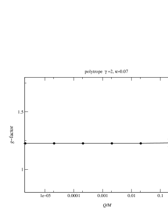
Figure 1: Variation of the $g$-factor as a function of the dimensionless ratio (total charge) / (gravitational mass), for a polytrope. Angular velocity $\Omega$ and baryon mass $M_{\rm B}$ are constant, being respectively equal to 200 Hz and $1.6M_{\odot}$. Error bars are given by the GRV2 test.

To calculate the $g$-factor of a given model, in addition to the choice of a particular equation of state, one has to set the three following parameters: the central density $n_{\rm B}(r=0)$ (or, equivalently, the central log-enthalpy $\left.\ln(e+p)/n_{\rm B}\right|_{r=0}$), the angular velocity $\Omega$ and the ratio between mass and charge densities $\chi$ (8).

3.1 Polytropes

In this part we choose the EOS to be a polytropic one, of the form (6.40) of reference [2]: $p=\kappa n_{\rm B}^{\gamma}$. We took $\gamma=2$ and $\kappa=0.07\rho_{\rm nuc}c^{2}/n_{\rm nuc}^{2}$, where nuclear density $\rho_{\rm nuc}=1.66\times 10^{17}{\rm kg/m^{3}}$ and $n_{\rm nuc}=0.1{\rm fm}^{-3}$. We first want to test the validity of our assumption neglecting electromagnetic forces in the equilibrium of the fluid. We computed a sequence of configurations increasing the total charge, at fixed angular velocity $\Omega=200$ Hz and fixed number of baryons (equivalent to 1.6 solar mass). Results for the $g$-factor (1) as a function of the dimensionless ratio $Q/M$ are displayed in figure 1, together with the errors given by the virial identities (see section 2.3). For $Q/M\lesssim 0.01$, $g$ is constant at $10^{-5}$ accuracy. For $Q/M\gtrsim 0.01$, $g$ starts to vary, but this variation remains within error bars, that become very important as $Q/M\to 1$. This indicates that the fact that we are neglecting electromagnetic forces in the equilibrium of the star induces an error that is lower than the numerical one, as long as $Q/M\lesssim 0.01$. It may be seen as a “low charge” approximation for our model and, within this approximation, we have checked with different equations of state (other polytropes, incompressible fluid EOS, strange matter EOS) that the $g$-factor would not depend on the charge. Let us say here that, although we are neglecting electromagnetic forces in the fluid equilibrium, we are taking the electromagnetic field into account in the sources of Einstein equations.

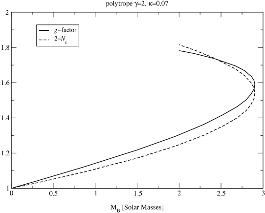
Figure 2: Variation of the $g$-factor and of the central lapse $N_{c}=N(r=0)$, as a function of baryon mass, for a polytrope. Angular velocity $\Omega=10$ Hz is kept constant.

The regime for which $Q/M>1$ does not seem realistic for a perfect fluid. Indeed, the repulsive Coulomb force acting on charged particles becomes comparable to the gravitational force and pressure. Therefore, there may not exist any stationary configuration for $Q/M$ too larger than 1: the electrostatic force would overcome the gravitational one and disperse particles. Moreover, Mustafa et al. [11] have shown that, in the case of a slowly rotating charged shell, when $Q/M>1$ there is no upper or lower bound on the value of the $g$-factor. Finally, in order to find an acceptable stationary solution for $0.01\lesssim Q/M<1$, one would have to satisfy both equations (7) and $j^{t}=\chi n_{\rm B}$. These are, in general, incompatible for a constant angular velocity $\Omega$ and one would have to allow for differential rotation of the fluid. This has not been done in our study and it would certainly be an improvement of our work. In the following, we will stay at $Q/M=10^{-3}$ an will consider that $g$ is independent of the total charge, in the low charge regime.

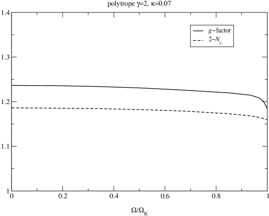
Figure 3: Variation of the $g$-factor and of the central lapse $N_{c}=N(r=0)$, as a function of the angular velocity, for a polytrope. The baryon mass $M_{\rm B}=1.6M_{\odot}$ is kept constant.

Now, we look at the variation of $g$, when the number of particles (the baryon mass $M_{\rm B}$) of the rotating polytrope is changed. Results for the $g$-factor are displayed in figure 2 (solid line), together with the value of the lapse $N$ at the centre of the star (dashed line). The parameter varying along both curves is the central density and we retrieve the well-known result of the existence of a maximal mass for those stars. Thus, the higher branch of each curve corresponds to unstable configurations. The Newtonian limit $g=1$ is recovered at low baryon masses, corresponding to weak gravitational field ($N_{c}\to 1$). In more relativistic regime, the $g$-factor follows roughly the variation of the central lapse, never reaching the value of 2 (corresponding to $N_{c}=0$), which corresponds to a charged black hole. The maximal value that could be reached (for an unstable configuration) was $g=1.8$, if only stable solutions are considered, then one has $g\leq 1.6$.

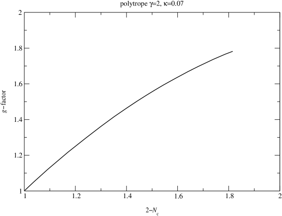
Figure 4: Variation of the $g$-factor as a function of the central lapse $N_{c}=N(r=0)$, for a polytrope. The angular velocity $\Omega=10$ Hz is kept constant.

The third parameter whose influence we want to study is the angular velocity $\Omega$. Therefore, at fixed number of particles in the star, and fixed total charge, we varied $\Omega$ from (almost) 0 to the maximal value, called Keplerian frequency ($\Omega_{\rm K}$), where the centrifugal force at the equator compensate the gravitational attraction (shedding limit). The variation of the $g$-factor as a function of $\Omega/\Omega_{\rm K}$, as well as that of a linear combination of the central lapse $2-N_{c}$ are displayed in figure 3. Both quantities show the same type of behaviour: they are decreasing functions, mainly near $\Omega\sim\Omega_{\rm K}$, but the overall change is relatively small, when compared to that of figure 2. We have explored here high angular velocities, without any “slow-rotation” assumption, but the influence of these high velocities seems rather small. We have checked at different masses, always obtaining the same kind of result. Here again, we see that $2-N_{c}$ and $g$ follow the same type of evolution, when varying $\Omega$. We therefore have plotted the $g$-factor, as a function of $2-N_{c}$ as shown in figure 4, when varying the central value of the density $n_{\rm B}(r=0)$, like in figure 2. Contrary to that figure, there is no sign of the maximal mass point, the $g$-factor being directly dependent on the strength of the gravitational field at the centre of the star. It seems that the gyromagnetic factor (1) might be another indicator of the strength of the gravitational field in self-gravitating objects: when gravity is weak (well described by Newtonian theory), we have $g\sim 1$; when the star is very compact (even unstable) $g$ takes its highest values. Finally, for a black hole, where gravity dominates over other forces, we have $g=2$.

3.2 Constant density models

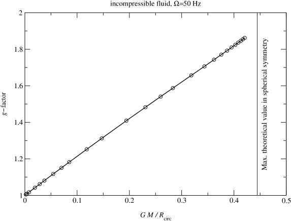
Figure 5: Variation of the $g$-factor as a function of the compaction parameter ${\cal C}=M/R_{\rm circ}$, at constant angular velocity $\Omega=50$ Hz, for an incompressible fluid. Circles show the model that have been computed. The vertical line at ${\cal C}=4/9$ corresponds to the maximal value of the compaction parameter for spherically symmetric stars (see [12]).

In order to study the dependence of the results of the previous section on the particular EOS, we first changed the values of $\gamma$ and $\kappa$. The results obtained were qualitatively the same as in previous section. Quantitatively, the trend described at the end of previous section (figure 4 and the following discussion), indicating that the $g$-factor be linked with the strength of the gravitational field in the star was retrieved. We found that the more compact the star, the higher the gyromagnetic factor. We checked this result with several other equations of state, described in Salgado et al. [9], as well as with the “strange quark matter” model (see Gourgoulhon et al. [10]), which is giving very compact objects. Still, none of these EOS allowed for a stable configuration with $g\gtrsim 1.8$.

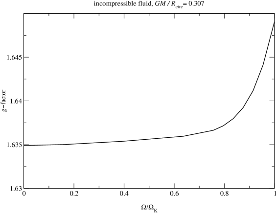
Figure 6: Variation of the $g$-factor as a function of the angular velocity, at constant compaction parameter ${\cal C}=M/R_{\rm circ}=0.307$ for an incompressible fluid.

Finally, we present here the limiting case of an incompressible fluid: the EOS is such that $n_{\rm B}$ and $e$ are constant throughout the star. Using this EOS in spherical symmetry, it can be shown (see, [12]) that it gives an upper limit on the gravitational redshift at the surface of the star, when comparing with other EOS. We here introduce a new dimensionless quantity called compaction parameter

$${\cal C}=\frac{M}{R_{\rm circ}},$$ (10)

with $R_{\rm circ}$ being defined by formula (9). In Newtonian theory, this is the gravitational potential at the surface of the star and ${\cal C}\ll 1$. On the other hand, for a Schwarzschild black hole ${\cal C}=0.5$ and, for relativistic stars $0\leq{\cal C}\leq 4/9$ (as derived by Buchdahl [12]). When considering charged objects the maximal value is slightly increased, as shown in Mak et al. [13]. In figure 5, we display the dependence of the gyromagnetic factor on this compaction parameter. As expected from previous results, we find that $g$ goes to 1, when $\cal C$ becomes very small (Newtonian limit). We could not reach the maximal theoretical value of the compaction parameter for spherical stars (4/9), due to the rotation and, perhaps, to the numerical algorithm (we look for a solution by iteration, starting with a flat metric). Nevertheless, we were able to get rather close to this limiting value, reaching the highest gyromagnetic factors for self-gravitating fluids, with $g\sim 1.86$. The striking feature is that the $g$-factor seems to be directly proportional to the compaction parameter $\cal C$ and, if one extrapolates the line to the maximal value of $\cal C$, one finds that the maximal value for the $g$-factor would be about 1.9, and certainly well below 2. Using only low charge objects, this value of 2 is linked with the collapse limit that cannot be reached with our stationary models.

It is now worth returning to the dependence of $g$ on the angular velocity $\Omega$. If we fix the value of $\cal C$ for the star, how does then gyromagnetic factor vary as a function of $\Omega$ ? The answer is displayed in figure 6, still in the case of an incompressible fluid. We see that the dependence is very small, only about one percent of variation between the non-rotating limit and the shedding one. Results shown in figure 3 can have a new interpretation: when $\Omega$ is increased, $\cal C$ decreases because of centrifugal forces that go against gravity and therefore make $R_{\rm circ}$ increase. Gravitational potential at the surface of the star decreases because of the rotation, the same being true for the gravitational field $N$ at the centre. The gyromagnetic factor indicates that, at high angular velocities, the star is less gravitationally bound. Comparing different models, equally bound, but with different rotation rates (figure 6), we see that the effect of rotation is small, and must act on the increase of $g$ through the addition of kinetic energy that contributes to the source terms of Einstein equations.

3.3 Comparison with previous works

There have been some studies of the gyromagnetic factor in general relativity, but none of them has considered physically consistent matter models. Much of interesting work has been done for slowly rotating charged shells, starting with that of Cohen et al. [14]. The study that may be most closely related to ours is that by Pfister and King [15], where the authors calculate explicitly the gyromagnetic factor of a charged mass shell in slow rotation approximation. The shell is infinitely thin and the authors match two exact solutions of the Einstein equations in vacuum across it. The properties of the energy-momentum tensor are then deduced from the matching of both metrics. The advantage of their solutions is that they were able to explore regimes with a very high charge and compaction parameter. Unfortunately, it is difficult to compare quantitatively their results with ours since one knows very little about the properties of shell matter which, apart from energy conditions, are not constrained. One might suppose that, in general, these shells are not behaving like perfect fluids. Qualitatively, both studies agree: for $Q/M\ll 1$ and taking into account energy conditions, Pfister and King find that $g$ varies between $\sim 1$, for a low compaction parameter, and 2 in the collapse limit. With a similar kind of problem, Mustafa et al. [11] found that $g$ could reach values very close to 2, for the charge-to-mass ratio less than unity and for the shell radius approaching the event horizon value.

Garfinkle and Traschen [16] have calculated the $g$-factor of a rotating massive loop of charged matter in the presence of a static charged black hole. They have found that, for large radii of the loop, $g$ tended to 1, whereas they found $g\to 2$ for the radius approaching the horizon. We retrieve (again qualitatively) the same results for our self-gravitating and three-dimensional objects: a loop at spatial infinity might be seen as undergoing a weak gravitational field, just like self-gravitating body with a low compaction parameter. Let us also mention here the very interesting work by Katz et al., who calculated the gyromagnetic ratio in a conformastationary metric [17]. These axially symmetric metrics can be seen as the external metrics for disc sources, made of charged dust. They show that in those discs, hoop tensions are always necessary to balance the centrifugal forces induced by the motion of the rotating dust. The model therefore correspond to non-perfect fluid, and they find $g=2$ (with our definition) for these metrics.

4 Conclusions

We have studied the dependence of the gyromagnetic ratio (1) of self-gravitating rotating fluids on their mass (number of particles), angular velocity and equation of state. We have used a physical model in which we make the assumption that the fluid is an insulator in uniform rotation, and we have neglected the electromagnetic forces acting on the equilibrium of the fluid (low charge approximation). These models have been solved numerically, with a code giving the solution in all space, which enabled us to get the value of $g$ with a high accuracy (better than $10^{-5}$) given by independent tests. We find that, with such “stars”, $g$ can never reach the value 2, characteristic of a charged rotating black hole. The maximal value that can be achieved in our study is lower than 1.9. This gap may be linked with the fact that we have neglected electromagnetic forces on hydrodynamic equilibrium and our study has therefore been restricted to low charge-to-mass ratios. But it might also be a result of that stationary relativistic stars, made of perfect fluid, cannot reach values of the compaction parameter $M/R$ close to 1/2. In that sense, the $g$-factor is a good indicator of the strength of the gravitational field in an insulating perfect fluid, but is little dependent on the angular velocity of the star. In our study, the value $g=2$ seems linked only with the black hole solution but, from other works, [14], [15] and [11], one can see that this may depend on the total charge of the system. An important improvement of our work would be to allow for any charge of the system, that is compatible with the stationarity assumption and therefore allow for differential rotation, which may open new possibilities.

References

References

- [1] Pfister H and King M 2003 Class. Quantum Grav.20 205
- [2] Bonazzola S, Gourgoulhon E, Salgado M and Marck J A 1993 Astron. Astrophys. 278 421
- [3] Bocquet M, Bonazzola S, Gourgoulhon E and Novak J 1995 Astron. Astrophys. 301 757
- [4] Cardall C, Prakash M and Lattimer J 2001 Astrophys. J. 554 322
- [5] Granclément P, Bonazzola S, Gourgoulhon E and Marck J A 2001 J. Comput. Phys. 170 231
- [6] Bonazzola S 1973 Astrophys. J. 182 335
- [7] Bonazzola S and Gourgoulhon E 1994 Class. Quantum Grav.11 1775
- [8] Gourgoulhon E and Bonazzola S 1994 Class. Quantum Grav.11 443
- [9] Salgado M, Bonazzola S, Gourgoulhon E and Haensel P 1994 Astron. Astrophys. 291 155
- [10] Gourgoulhon E, Haensel P, Livine R, Paluch E, Bonazzola S and Marck J A 1999 Astron. Astrophys. 349 851
- [11] Mustafa E, Cohen J M and Pechenick K R 1987 Int. J. Theor. Phys. 26 1189
- [12] Buchdahl H A 1959 Phys. Rev.116 1027
- [13] Mak M K, Dobson P N and Harko T 2001 Europhys. Lett. 55 310
- [14] Cohen J M, Tiomno J and Wald R M 1973 Phys. Rev.D 7 998
- [15] Pfister H and King M 2002 Phys. Rev.D 65 084033
- [16] Garfinkle D and Traschen J 1990 Phys. Rev.D 42 419
- [17] Katz J, Bičák J and Lynden-Bell D 1999 Class. Quantum Grav.16 4023