Simultaneity and the Concept of ‘Particle’

Abstract

The history of the particle concept is briefly reviewed, with particular emphasis on the ‘foliation dependence’ of many particle creation models, and the possible connection between our notion of particle and our notion of simultaneity. It is argued that the concept of ‘radar time’ (originally introduced by Sir Hermann Bondi in his work on k-calculus) provides a satisfactory concept of ‘simultaneity’ for observers in curved spacetimes. This is used to propose an observer-dependent particle interpretation, applicable to an arbitrary observer, depending solely on that observers motion and not on a choice of coordinates or gauge. This definition is illustrated with application to non-inertial observers and simple cosmologies, demonstrating its generality and its consistency with known cases.

1 Introduction

In this conference we have heard illuminating discussions of various aspects of the role of time in physics, and the conceptual tension that often surrounds it. One well-known tension is between the ‘effectively absolute’ role that time plays in quantum mechanics, and the role it plays in general relativity, where it is just one coordinate in a covariant theory. My contribution to these proceeding will discuss the problem of particle creation in gravitational backgrounds, and in accelerating reference frames. In so doing I hope to shed some light on the aforementioned tension, and also to describe a fascinating connection that exists between our concept of simultaneity, and our concepts of ‘particle’ and ‘vacuum’.

The first prediction of particle creation in gravitational backgrounds came in 1939 when Schrödinger[1] predicted that if the universe is expanding then “it would mean production of matter merely by its expansion”. This prediction was readressed in detail by Parker[2, 3, 4] in the late 60’s. However, gravitational particle creation first hit the headlines in 1975, with the discovery of Hawking radiation from black holes [5]. Perhaps an even more intriguing discovery was made later that year, by Unruh[6] and independently by Davies[7]. They showed that an observer who accelerates uniformly through flat empty space will also observe a thermal bath of particles, at a temperature given by their acceleration. This means that a state which is empty according to an inertial observer will not be empty according to an accelerating observer, and hence it demonstrates that the concept of ‘vacuum’ (and hence of ‘particle’) must be observer-dependent. To see how these predictions could arise, consider a globally hyperbolic spacetime, and for definiteness, consider massive Dirac fermions. Then we have a field operator $\hat{\psi}(x)$ satisfying[8, 9]:

$$(i\gamma^{\mu}\nabla_{\mu}-m)\hat{\psi}(x)=0$$ (1)

where $\{\gamma^{\mu},\gamma^{\nu}\}=2g^{\mu\nu}$, $\nabla_{\mu}\psi\equiv\partial_{\mu}\psi+\Gamma_{\mu}\psi$ and $\Gamma_{\mu}=\frac{1}{4}\gamma_{\nu}\nabla_{\mu}\gamma^{\nu}$ is the spin connection. Since no interactions are present then we can expand $\hat{\psi}(x)$ in terms of a complete set of normal modes as:

$$\Longrightarrow\hat{\psi}(x)=\sum_{i}\{u_{i}(x)a_{i}+v_{i}(x)b^{\dagger}_{i}\}$$ (2)

However, these modes are no longer simple plane waves, so it is no longer obvious which modes should be put with the $a_{i}$ operators and interpreted as particle modes, and which should be put with the $b_{i}^{\dagger}$ operators and interpreted as antiparticle modes. Two choices must be made. The ‘in’ modes $\{u_{i,\rm{in}},v_{i,\rm{in}}\}$, chosen to represent particle/antiparticle modes at early times, determine the ‘in’ vacuum $|0_{\rm{in}}\rangle$ by the requirement:

$$a_{i,\rm{in}}|0_{\rm{in}}\rangle=0=b_{i,\rm{in}}|0_{\rm{in}}\rangle$$

The ‘out’ modes $\{u_{i,\rm{out}},v_{i,\rm{out}}\}$ determine the ‘out’ number operator

$$\hat{N}_{\rm{out}}=\sum_{i}\{a^{\dagger}_{i,\rm{out}}a_{i,\rm{out}}+b^{\dagger}_{i,\rm{out}}b_{i,\rm{out}}\}$$

By expanding the ‘out’ modes in in terms of the ‘in’ modes we obtain:

$$a_{i,\rm{out}} =\sum_{j}\{\alpha_{ij}a_{j,\rm{in}}+\beta_{ij}b^{\dagger}_{j,\rm{in}}\}$$ (3)

$$b_{i,\rm{out}} =\sum_{j}\{\gamma_{ij}^{*}a^{\dagger}_{j,\rm{in}}+\epsilon_{ij}^{*}b_{j,\rm{in}}\}$$ (4)

The number of ‘out’ particles in the ‘in’ vacuum is then given by:

$$\langle 0_{\rm{in}}|\hat{N}_{\rm{out}}|0_{\rm{in}}\rangle=Trace(\mbox{\boldmath$\beta$}\mbox{\boldmath$\beta$}^{\dagger}+\mbox{\boldmath$\gamma$}\mbox{\boldmath$\gamma$}^{\dagger})$$ (5)

hence describing particle creation. The task of describing particle creation then boils down to the question: How do we choose the ‘in’ and ‘out’ modes?

There are a large variety of methods proposed for this choice (see for instance the common texts[10, 11] and the references therein), based on adiabatic expansions, conformal symmetry, killing vectors, the diagonalisation of a suitable Hamiltonian, or many other methods. Broadly speaking these methods are limited by one of two drawbacks. Either they require the spacetime to possess certain desirable symmetries (deSitter, Killing vectors, conformal symmetries etc), or they give results which depend on an arbitrary foliation of spacetime into ‘space’ and ‘time’. Meanwhile, although a choice of observer often motivates the choice of foliation (such as in the Unruh effect), there is no systematic prescription for linking the chosen observer to the chosen foliation.

Many of these drawbacks can be avoided by introducing a model particle detector[6, 10, 12, 13]. This provides an operational particle concept, which directly incorporates the observers motion. However, it can not be used to define the particle/antiparticle modes, for a number of reasons. Firstly, because a detector only counts particles on its trajectory, so could not for instance categorize the emptiness of a state. More importantly, it would be circular. Provided a particle detector is anything that detects particles, a particle cannot also be “anything detected by a particle detector”. Even if we stick only to ‘tried and tested’ detector models[6, 14], then the question arises “what were they tested against?” - we must have in mind a concept of particle before fashioning a concept of detector. (In the case of fermions there are also technical difficulties[12, 13, 15], meaning that the predictions of current detector models are not always proportional to the number of particles present, even for inertial detectors in electro-magnetic fields.)

In this article we offer a resolution to these difficulties[16, 17, 18] which builds on the so-called ‘Hamiltonian diagonalisation’ prescription[19, 20, 21, 22]; a method criticized in the past[23] for its reliance on an arbitrarily chosen foliation of spacetime (time coordinate). Our resolution lies in using the concept of ‘radar time’ (originally introduced by Sir Hermann Bondi[24, 25, 26] in his work on k-calculus) to uniquely assign a foliation of spacetime to any given observer. The result is a particle interpretation which depends only on the motion of the observer, and on the background present, and which generalizes Gibbons’ definition[27] to arbitrary observers and non-stationary spacetimes. It also facilitates the definition of a number density operator, allowing us to calculate not just the total asymptotic particle creation, but also to say (with definable precision) where and when these particles were ‘created’.

Given the central role that radar time will play in this particle interpretation, the next Section is devoted to describing radar time, while Section 3 describes the application of radar time to an arbitrary observer in 1+1 Dimensional Minkowski Space. The observer-dependent particle interpretation is defined and discussed in Section 4. In Section 5 we return to 1+1 Dimensional Minkowski space, and describe the massless Dirac Vacuum as seen by an arbitrarily moving observer. Conclusions are presented in Section 6.

2 Radar Time

Consider an observer traveling on path $\gamma:x^{\mu}=x^{\mu}(\tau)$ with proper time $\tau$, and define:

$$\tau^{+}(x) \equiv\mbox{ (earliest possible) proper time at which a null geodesic leaving}$$

point $$x \gamma$$ could intercept .

$$\tau^{-}(x) \equiv\mbox{ (latest possible) proper time at which a null geodesic could}$$

leave $$\gamma x$$, and still reach point .

$$\tau(x) \equiv{\textstyle\frac{1}{2}}(\tau^{+}(x)+\tau^{-}(x))\hskip 28.45274pt=\mbox{ `radar time'.}$$

$$\rho(x) \equiv{\textstyle\frac{1}{2}}(\tau^{+}(x)-\tau^{-}(x))\hskip 28.45274pt=\mbox{ `radar distance'.}$$

$$\Sigma_{\tau_{0}} \equiv\{x:\tau(x)=\tau_{0}\}=\mbox{ observer's `hypersurface of simultaneity at time $\tau_{0}$'. }$$

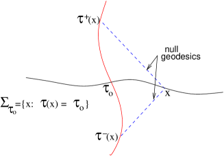
Figure 1: Schematic of the definition of ‘radar time’ $\tau(x)$.

This is a simple generalization of the definition made popular by Bondi in his work on special relativity and k-calculus[24, 25, 28]. It can be applied to any observer in any spacetime. We can also define the ‘time-translation’ vector field:

$$k_{\mu}(x)\equiv\frac{\frac{\partial\tau}{\partial x^{\mu}}}{g^{\sigma\nu}\frac{\partial\tau}{\partial x^{\sigma}}\frac{\partial\tau}{\partial x^{\nu}}}$$ (6)

This represents the perpendicular distance between neighboring hypersurfaces of simultaneity, since it is normal to these hypersurfaces and it satisfies $k^{\mu}(x)\frac{\partial\tau}{\partial x^{\mu}}=1$. Radar time is independent of the choice of coordinates, and is single valued in the observers causal envelope (the set of all spacetime points with which the observer can both send and receive signals). An affine reparametrisation of the observers worldline leads only to a relabeling of the same foliation, such that the radar time always agrees with proper time on the observer’s path. It is invariant under ‘time-reversal’ - that is, under reversal of the sign of the observer’s proper time.

We now illustrate these properties with a simple class of examples; observers in 1+1 Dimensional Minkowski space. Some simple cosmological examples are presented elsewhere[18].

3 Arbitrary Observer in 1 + 1 Dimensions

Let the observers worldline be described by

$$x^{\pm}\equiv t\pm x=x^{\pm}_{\lambda}(\tau_{\lambda})=\int^{\tau_{\lambda}}e^{\pm\alpha(\tau)}{\rm d}\tau$$

where $\tau_{\lambda}$ is the observers proper time, and $\alpha(\tau_{\lambda})$ is the observers ‘rapidity’ at time $\tau_{\lambda}$. $e^{\alpha(\tau_{\lambda})}$ is the obvious time-dependent generalization of the ‘k’ of Bondi’s k-calculus[24, 25, 28]. The observers acceleration is $a(\tau_{\lambda})=\frac{d\alpha}{d\tau_{\lambda}}$. The observers worldline is completely specified by the choice of origin (i.e. $x^{\mu}(0)$) and the rapidity function $\alpha(\tau_{\lambda})$, or by the choice of origin, the initial velocity, and the function $a(\tau_{\lambda})$.

It is straightforward to show that the coordinates $\tau^{\pm}=\tau\pm\rho$ are given by:

$$x^{\pm}=x^{\pm}_{\lambda}(\tau^{\pm})$$

while the metric in these coordinates is:

$${\rm d}s^{2}=e^{(\alpha(\tau^{+})-\alpha(\tau^{-}))}({\rm d}\tau^{2}-{\rm d}\rho^{2})$$

We see that the radar coordinates are obtained from the Minkowski coordinates simply by rescaling along the null axes. The ‘time-translation vector field’ [18, 17] is simply $k^{\mu}\frac{\partial}{\partial x^{\mu}}=\frac{\partial}{\partial\tau}$, while the hypersurfaces $\Sigma_{\tau}$ are hypersurfaces of constant $\tau$.

As a useful consistency check, consider an inertial observer with a velocity $v$ relative to our original frame. Then $\alpha$ is constant, and $x^{\pm}_{\lambda}(\tau_{\lambda})=e^{\pm\alpha}\tau_{\lambda}$. The coordinates $\tau^{\pm}$ are hence given by $\tau^{\pm}=e^{\mp\alpha}x^{\pm}$ so:

$$\tau={\textstyle\frac{1}{2}}(e^{-\alpha}x^{+}+e^{\alpha}x^{-})=\frac{t-vx}{\sqrt{1-v^{2}}},\hskip 28.45274pt\rho={\textstyle\frac{1}{2}}(e^{-\alpha}x^{+}-e^{\alpha}x^{-})=\frac{x-vt}{\sqrt{1-v^{2}}}$$

The radar coordinates of an inertial observer are just the coordinates of their rest frame, as expected.

3.1 Constant Acceleration

The simplest nontrivial case is constant acceleration. In this case $\alpha(\tau)=a\tau$, and we have $x^{\pm}_{\lambda}(\tau_{\lambda})=\pm a^{-1}e^{\pm a\tau_{\lambda}}$ which gives:

$$\tau =\frac{1}{2a}\log\left(\frac{x+t}{x-t}\right)\hskip 56.9055pt\rho=\frac{1}{2a}\log\left(a^{2}(x^{2}-t^{2})\right)$$ (7)

$${\rm d}s^{2} =e^{2a\rho}({\rm d}\tau^{2}-{\rm d}\rho^{2})$$ (8)

These are Rindler coordinates, which cover only region U of Figure 2, as expected. The hypersurfaces of constant $\tau$ are given by $t_{\tau_{0}}(x)=x\tanh(a\tau_{0})$.

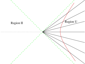
Figure 2: Hypersurfaces of simultaneity of a uniformly accelerating observer.

3.2 Gradual Turnaround Cases

Consider now an observer (Barbara say) who accelerates uniformly for $|\tau_{\lambda}|<\tau_{c}$, but is otherwise inertial. Then $\alpha(\tau_{\lambda})=a\tau_{\lambda}$ for $|\tau_{\lambda}|<\tau_{c}$ and $=\pm a\tau_{c}$ for $\tau_{\lambda}>\tau_{c}$ or $<-\tau_{c}$ respectively.

Figure LABEL:fig1(A). Barbara’s hypersurfaces of constant $\tau$.

Figure LABEL:fig1(B). Barbara’s instantaneous rest frames.

The hypersurfaces of simultaneity for this observer are shown in Figure 3 (A). For comparison we have included the standard ‘instantaneous rest frame’ in Figure 3 (B). The instantaneous rest frame suffers from being triple valued to the observers left. It is also sensitively dependent on the small-scale details of Barbara’s trajectory. Consider for instance a small deviation of Barbara’s trajectory, like the small dotted line in the turnaround point of Figures 3 (A) and 3 (B). In figure 3 (B) this has serious effects - Barbara now assigns five times to events far to her left, and three to events far to her right! In 3 (A) however, this change causes only a small change in the times assigned to events in the vicinity of the points marked $C$.

A similar example is that of an observer with trajectory given by:

$$x^{\pm}_{\lambda}(\tau_{\lambda})=\int_{0}^{\tau_{\lambda}}e^{\pm a\tau_{c}\tanh(\tau/\tau_{c})}{\rm d}\tau$$

This observer has acceleration $a(\tau)=a\cosh^{-2}(\tau/\tau_{c})$, so is uniformly accelerating for $|\tau|<<\tau_{c}$ and inertial for $|\tau|>>\tau_{c}$. We will return to this example shortly.

4 An Observer-Dependent Particle Interpretation

Consider again the field operator:

$$\hat{\psi}(x)=\sum_{i}\{u_{i,\rm{in}}(x)a_{i,\rm{in}}+v_{i,\rm{in}}(x)b_{i,\rm{in}}^{\dagger}\}$$ (9)

and the state $|\rm{in}\rangle$ defined by $a_{i,\rm{in}}|\rm{in}\rangle=0=b_{i,\rm{in}}|\rm{in}\rangle$. We will consider the time-dependent particle content of this state, as measured by an observer O. We mentioned in the introduction that this definition stems from the diagonalisation of a suitable Hamiltonian. The Hamiltonian in question is:

$$\hat{H}(\tau) =\int_{\Sigma_{\tau}}\sqrt{-g}\ k^{\mu}T_{\mu\nu}(\hat{\psi},\hat{\psi}){\rm d}\Sigma^{\nu}$$ (10)

$$\mbox{where }T_{\mu\nu}(\psi,\phi) ={\textstyle\frac{1}{2}}i[\bar{\psi}\gamma_{(\mu}\nabla_{\nu)}\phi-(\nabla_{(\mu}\bar{\psi})\gamma_{\nu)}\phi]$$ (11)

$T_{\mu\nu}(\hat{\psi},\hat{\psi})$ is the (unregularised) stress-energy tensor for Dirac fermions[10]. Diagonalising this Hamiltonian[22] entails expanding $\hat{\psi}$ as:

$$\hat{\psi}(x) =\sum_{i}u_{i,\tau_{0}}(x)a_{i,\tau_{0}}+\sum_{i}v_{i,\tau_{0}}(x)b^{\dagger}_{i,\tau_{0}}+\sum_{i}w_{i,\tau_{0}}(x)c_{i,\tau_{0}}$$ (12)

$$=\hat{\psi}^{(+)}_{\tau_{0}}(x)+\hat{\psi}^{(-)}_{\tau_{0}}(x)+\hat{\psi}^{(0)}_{\tau_{0}}(x)$$ (13)

and choosing these modes such that the Hamiltonian becomes:

$$\hat{H}(\tau_{0})=\sum_{ij}h^{(+)}_{ij}(\tau_{0})a^{\dagger}_{i,\tau_{0}}a_{j,\tau_{0}}-\sum_{ij}h^{(-)}_{ij}(\tau_{0})b_{i,\tau_{0}}b^{\dagger}_{j,\tau_{0}}$$ (14)

where the matrices $\mbox{\boldmath$h$}^{(\pm)}$ are positive definite. To consider the content of this requirement, it is convenient to define the ‘1st quantized Hamiltonian’ $\hat{H}_{1}(\tau)$ (on the space of finite-norm solutions of the Dirac equation) by:

$$\langle\psi|\hat{H}_{1}(\tau)|\phi\rangle=\int_{\Sigma_{\tau}}\sqrt{-g}\ k^{\mu}T_{\mu\nu}(\psi,\phi){\rm d}\Sigma^{\nu}$$

Then equation (14) requires that $\{u_{i,\tau_{0}}(x)\}$ span the positive spectrum of $\hat{H}_{1}(\tau_{0})$, $\{v_{i,\tau_{0}}(x)\}$ span the negative spectrum of $\hat{H}_{1}(\tau_{0})$, and $\{w_{i,\tau_{0}}(x)\}$ span the null space of $\hat{H}_{1}(\tau_{0})$. The $w_{i,\tau_{0}}(x)$ will generally be states of compact support outside the causal envelope of the observer. Having defined $\hat{\psi}^{(\pm)}(x)$ and $\hat{\psi}^{(0)}(x)$ by this requirement, we can now define the particle number operator on $\Sigma_{\tau_{0}}$, $\hat{N}^{+}_{\tau_{0}}$ by:

$$\hat{N}^{+}_{\tau_{0}}=\int_{\Sigma_{\tau_{0}}} \sqrt{-g}\ \bar{\hat{\psi}}^{(+)}_{\tau_{0}}\gamma^{\mu}\hat{\psi}^{(+)}_{\tau_{0}}{\rm d}\Sigma_{\mu}\hskip 14.22636pt=\int_{\Sigma_{\tau_{0}}}\sqrt{-g}\ \hat{J}^{\mu(+)}{\rm d}\Sigma_{\mu}$$ (15)

where $$\hat{J}^{\mu(+)}=\bar{\hat{\psi}}^{(+)}_{\tau(x)}\gamma^{\mu}\hat{\psi}^{(+)}_{\tau(x)}$$ (16)

For any state and any chosen observer, the field $\langle J^{\mu(+)}\rangle$ is a covariant vector field, which can be interpreted as describing the ‘flow of particles’ as seen by this observer. $\hat{J}^{\mu(+)}{\rm d}\Sigma_{\mu}$ represents the number of particles in ${\rm d}\Sigma_{\mu}$. Similarly, the antiparticle number operator is given by:

$$\hat{N}^{-}_{\tau_{0}}=-:\int_{\Sigma_{\tau_{0}}} \sqrt{-g}\ \bar{\hat{\psi}}^{(-)}_{\tau_{0}}\gamma^{\mu}\hat{\psi}^{(-)}_{\tau_{0}}{\rm d}\Sigma_{\mu}:\hskip 14.22636pt=\int_{\Sigma_{\tau_{0}}}\sqrt{-g}\ \hat{J}^{\mu(-)}{\rm d}\Sigma_{\mu}$$ (17)

where $$\hat{J}^{\mu(-)}=-:\bar{\hat{\psi}}^{(-)}_{\tau(x)}\gamma^{\mu}\hat{\psi}^{(-)}_{\tau(x)}:$$ (18)

The normal-ordering is with respect to the observers particle interpretation at the time of measurement (i.e. the $b_{i,\tau}$). These operators allow the observer to calculate the total number of particles/antiparticles on $\Sigma_{\tau}$ for all $\tau$, and to determine how this particle content is distributed throughout $\Sigma_{\tau}$. Although the total number operator $\hat{N}_{\tau}=\hat{N}^{+}_{\tau}+\hat{N}^{-}_{\tau}$ is necessarily non-local (no local operator could possibly be consistent with the Unruh effect) it will generally be effectively local[16, 17] on scales larger than the Compton length $\lambda_{c}=\frac{h}{mc}$ of the particle concerned. Equating expressions (9) and (12) for $\hat{\psi}(x)$ gives:

$$a_{i,\tau_{0}} =\sum_{j}\{\langle u_{i,\tau_{0}}|u_{j,\rm{in}}\rangle a_{j,\rm{in}}+\langle u_{i,\tau_{0}}|v_{j,\rm{in}}\rangle b^{\dagger}_{j,\rm{in}}\}$$ (19)

$$b_{i,\tau_{0}} =\sum_{j}\{\langle v_{i,\tau_{0}}|u_{j,\rm{in}}\rangle^{*}a_{j,\rm{in}}+\langle v_{i,\tau_{0}}|v_{j,\rm{in}}\rangle^{*}b^{\dagger}_{j,\rm{in}}\}$$ (20)

which allows us to deduce for instance:

$$\langle\rm{in}|\hat{N}^{+}_{\tau_{0}}|\rm{in}\rangle =\rm{Trace}(\mbox{\boldmath$\beta$}\mbox{\boldmath$\beta$}^{\dagger})$$ (21)

$$\langle\rm{in}|\hat{N}^{-}_{\tau_{0}}|\rm{in}\rangle =\rm{Trace}(\mbox{\boldmath$\gamma$}\mbox{\boldmath$\gamma$}^{\dagger})$$ (22)

$$\mbox{ where }\beta_{ij}(\tau_{0})\equiv\langle u_{i,\tau_{0}}|v_{j,\rm{in}}\rangle\hskip 28.45274pt \mbox{and }\hskip 14.22636pt\gamma_{ij}(\tau_{0})\equiv\langle v_{i,\tau_{0}}|u_{j,\rm{in}}\rangle$$ (23)

as in equation (5). Note that, in the presence of horizons, the observer $O$ cannot define a unique ‘vacuum state’ at any time $\tau_{0}$. All he can say is that “a state $|0,\tau_{0}\rangle$ is vacuum throughout $\Sigma_{\tau_{0}}$” if:

$$a_{i,\tau_{0}}|0,\tau_{0}\rangle=0=b_{i,\tau_{0}}|0,\tau_{0}\rangle$$

for all $i$. This condition is not unique, since we have said nothing about $c_{i,\tau_{0}}|0,\tau_{0}\rangle$. This is a natural limitation however; since $O$ cannot communicate with points outside his causal envelope, we can’t expect him to be able to determine particle content in such regions.

Although we have specified the ‘out’ modes $\{u_{i,\tau},v_{i,\tau}\}$ for all possible ‘out times’, we have not yet discussed the choice of ‘in’ modes $\{u_{i,\rm{in}},v_{i,\rm{in}}\}$. This choice is largely a question of convenience, and depends on what state we wish to consider the properties of. In the absence of particle horizons (when $\hat{\psi}^{(0)}=0$) we may wish the ‘in’ state to be our observers ‘in-vacuum’ $|0,\tau_{\rm{in}}\rangle$ prepared at some ‘in’ time $\tau_{\rm{in}}$. Alternatively, we may wish that the state $|\rm{in}\rangle$ be prepared by someone other than the observer. This will be the case shortly, where the content of the inertial vacuum will be studied by an accelerating observer. Or we may wish (as is common in cosmological applications) to consider a state $|\rm{in}\rangle$ which is never considered ‘empty’ by any observer, but is instead justified by symmetry considerations[10].

5 The Massless Dirac Vacuum in 1+1 Dimensions

As a concrete example of these definitions, consider now the massless Dirac vacuum $|0_{M}\rangle$ of flat 1+1 Dimensional Minkowski space, as measured by an arbitrarily moving observer (more detail is presented elsewhere[31]). Then the ‘in’ modes are the plane wave states, which can be written in the massless case as:

$$u_{p,\pm,\rm{in}}(x)=e^{-ipx^{\mp}}\phi_{\pm},\hskip 28.45274ptv_{p,\pm,\rm{in}}(x)=e^{ipx^{\mp}}\phi_{\pm}\hskip 28.45274pt\mbox{ for }p>0$$ (24)

where the subscript $\pm$ denotes forward/backward moving modes, and the basis spinors $\phi_{\pm}$ satisfy $\bar{\gamma}_{1}\bar{\gamma}_{0}\phi_{\pm}=\pm\phi_{\pm}$ where $\bar{\gamma}_{\mu}$ are the flat space Dirac matrices in 1+1 Dimensions. It can be shown[31] that the modes:

$$u_{\omega,\pm,O}=e^{\pm{\textstyle\frac{1}{2}}\alpha(\tau^{\mp})}e^{-i\omega\tau^{\mp}}\phi_{\pm}\hskip 28.45274ptv_{\omega,\pm,O}=e^{\pm{\textstyle\frac{1}{2}}\alpha(\tau^{\mp})}e^{i\omega\tau^{\mp}}\phi_{\pm}\hskip 28.45274pt\mbox{ for }\omega>0$$ (25)

diagonalise $\hat{H}(\tau)$ for all $\tau$. Substituting (24) and (25) into (23) and calculating the integral over $p>0$ that is implicit in the Trace, gives:

$$(\beta\beta^{\dagger})_{\omega\omega^{\prime},\pm}=2\int_{-\infty}^{\infty} {\rm d}\tau_{a}e^{-i\omega_{d}\tau_{a}}\int_{0}^{\infty}{\rm d}\tau_{d}\sin(\omega_{a}\tau_{d})g_{\pm}(\tau_{a},\tau_{d})\hskip 14.22636pt=(\gamma\gamma^{\dagger})_{\omega\omega^{\prime},\pm}^{*}$$ (26)

$$\mbox{ where }g_{\pm}(\tau_{a},\tau_{d}) =\frac{1}{\tau_{d}}-\frac{\exp\left(\frac{\mp 1}{2}(\alpha(\tau_{a}+\tau_{d}/2)+\alpha(\tau_{a}-\tau_{d}/2))\right)}{\int_{-\tau_{d}/2}^{\tau_{d}/2}\exp(\mp\alpha(\tau_{a}+\tau)){\rm d}\tau}$$ (27)

$$\omega_{a} ={\textstyle\frac{1}{2}}(\omega+\omega^{\prime})\hskip 14.22636pt\mbox{ and }\hskip 14.22636pt\omega_{d}=\omega^{\prime}-\omega$$ (28)

From these we can deduce that[31] the distribution $n^{+}_{F}(x)$ of forward moving particles exactly matches the distribution of forward moving antiparticles, and is given by:

$$n_{F}(\tau^{-}) =\int_{-\infty}^{\infty}\frac{{\rm d}\tau}{2\pi\tau}g_{+}(\tau^{-}+\tau,\tau)\hskip 14.22636pt=\int_{0}^{\infty}\frac{{\rm d}\omega_{a}}{2\pi}n_{F,\omega}(\tau^{-})$$ (29)

$$\mbox{where }n_{F,\omega}(\tau^{-}) =\int_{-\infty}^{\infty}{\rm d}\tau_{a}\ \frac{\sin[\omega(\tau^{-}-\tau_{a})]}{\pi(\tau^{-}-\tau_{a})}\int_{0}^{\infty}{\rm d}\tau_{d}\ \sin(\omega\tau_{d})g_{+}(\tau_{a},\tau_{d})$$ (30)

This is a function only of $\tau^{-}=\tau-\rho$, as would be expected for forward-moving massless particles. It is defined such that $n_{F}(\tau^{-}){\rm d}\rho$ gives the number of particles within ${\rm d}\rho$ of the point $(\tau,\rho)$. The function $n_{F,\omega}(\tau^{-})$ can be interpreted as the frequency distribution of forward moving particles/antiparticles at the point $\tau^{-}$. Equation (30), together with (27),expresses this distribution anywhere in the spacetime, directly in terms of the observers rapidity. Similarly, the spatial distribution of backward-moving particles matches that of backward moving antiparticles, and can be defined by $n_{B}(\tau^{+})=\int_{0}^{\infty}\frac{{\rm d}\omega}{2\pi}n_{B,\omega}(\tau^{+})$ where the expressions for $n_{B,\omega}(\tau^{+})$ and $n_{B}(\tau^{+})$ are as above, but with $g_{+}$ replaced with $g_{-}$ and $\tau^{-}$ replaced with $\tau^{+}$. Notice that if the observers worldline is time-symmetric about $\tau_{\lambda}=0$ then $\alpha(-\tau_{\lambda})=-\alpha(\tau_{\lambda})$ which gives $n_{F,\omega}(\tau^{\prime})=n_{B,\omega}(-\tau^{\prime})$ for all $\tau^{\prime}$. On the hypersurface $\tau=0$ for instance, where $\tau^{\pm}=\pm\rho$ this implies that the distribution of forward moving particles exactly matches that of backward moving particles. On the observers worldline on the other hand, the distribution of forward moving particles is the time-reverse of that for backward moving particles.

As a consistency check, consider again an inertial observer. Then $\alpha$ is constant, so $g_{\pm}(\tau_{a},\tau_{d})=0$, and the particle content is everywhere zero, as expected. We now consider other examples.

5.1 Constant Acceleration

For a uniformly accelerating observer we have:

$$g_{+}(\tau_{a},\tau_{d})=g_{-}(\tau_{a},\tau_{d})=\frac{1}{\tau_{d}}-\frac{a}{2\sinh\left(\frac{a\tau_{d}}{2}\right)}$$

which is independent of $\tau_{a}$. Hence the forward and backward moving particles are each distributed uniformly in $\rho$ for all $\tau$, and the frequency distribution is everywhere given by:

$$n_{F,\omega} =n_{B,\omega}=2\int_{0}^{\infty}d\tau_{d}\ \sin(\omega\tau_{d})\left(\frac{1}{\tau_{d}}-\frac{a}{2\sinh\left(\frac{a\tau_{d}}{2}\right)}\right)$$ (31)

$$=\frac{2\pi}{1+e^{\frac{2\pi\omega}{a}}}$$ (32)

which is a thermal spectrum at temperature $T=\frac{a}{2\pi k_{B}}$, as expected.

Figure LABEL:fig2(A). $n_{\omega}(\rho)/a$ as a function of $a\rho$, for $m=a$ and $\omega=a/4$ (lowest curve), $a$, and $4a$ (most oscillatory curve).

Figure LABEL:fig2(B). $n(\rho)/a$ as a function of $a\rho$, for $m=a/10$ (right curve), $a$ and $10a$ (left curve).

For comparison, briefly consider the case of massive fermions in 1+1 Dimensions (which no longer decompose into forward/backward moving modes). In this case the spatially averaged frequency distribution[8, 12, 32, 18] is as in (32), but the massive particles are no longer distributed uniformly in $\rho$ (although the distribution is completely independent of $\tau$). Nor is the spatial distribution independent of $\omega$. Figure 4 shows the spatial distribution of Rindler particles in this case[18]. Figure 4 (A) shows $n_{\omega}(\rho)/a$ as a function of $a\rho$ for $m=a$ and $\omega=a/4$ (lowest curve), $a$, and $4a$ (most oscillatory curve), while Figure 4 (B) shows $n(\rho)/a$ as a function of $a\rho$, for $m=a/10$ (right curve), $a$ and $10a$ (left curve). These can be understood by considering that these particles see an ‘effective mass gap’ of $2me^{a\rho}$. Each frequency penetrates to a value of $\rho$ for which $me^{a\rho}\sim\omega$. Changing the ratio $m/a$ is equivalent to a translation in $\rho$. We see that in general the particle number density is uniform to the observer’s left and negligible to the observer’s right, with the transition happening at $\rho\sim\frac{1}{a}\log\left(\frac{a}{m}\right)$. As $m\rightarrow 0$ this transition point goes to $\infty$, reproducing the spatial uniformity of the massless limit. However, for non-zero $m$ and realistic accelerations, the particle density is small even at low $\rho$ (where it is $\propto a$), while the transition to a negligible density occurs far to the observer’s left.

5.2 Gradual Turnaround Observer

Returning to the massless case, consider now the observer with acceleration

$$a(\tau_{\lambda})=a\cosh^{-2}\left(\frac{\tau_{\lambda}}{\tau_{c}}\right)$$

Their rapidity is $\alpha(\tau_{\lambda})=a\tau_{c}\tanh(\tau/\tau_{c})$. They are accelerating uniformly for $|\tau|<<\tau_{c}$, but are inertial at asymptotically early and late times (with velocity $\pm\tanh(a\tau_{c})$). There are no particle horizons in this case; the observers causal envelope covers the whole spacetime. By substituting the rapidity into equation (27) we immediately obtain the spatial distribution of forward or backward moving particles. At time $\tau=0$ these distributions are equal. They are shown in Figure 5, as a function of $a\rho$ for $a\tau_{c}=1$ (bottom curve), $3,10,30,100$ and $\infty$ (top line). As $\tau_{c}$ increases the particle density increases, and approaches the spatial uniformity of the $\tau_{c}\rightarrow\infty$ limit.

Figure 5: $n_{F,B}(\rho)/a$ as a function of $a\rho$ for $\tau=0$ and $a\tau_{c}=1$ (bottom curve), $3,10,30,100$ and $\infty$ (top curve).

In Figure 6 we have shown the frequency distribution $n_{F,\omega}(\rho)$ of forward-moving particles, as a function of $\omega/a$ for $\tau=0$. In Figure 6 (A) we have $\rho=0$ and $a\tau_{c}=3,10,30$ and $\infty$. We can clearly see that the distribution approaches thermal as $\tau_{c}$ is increased. In Figure 6 (B) $a\tau_{c}=10$ and $a\rho=\pm 10$. We have also included a plot corresponding to a thermal spectrum appropriate to a constant acceleration of $a\cosh^{-2}(1)$. The difference between the actual spectrum and the thermal spectrum is more significant here. Since $n_{F,B}$ depend only on $\tau^{\pm}$ respectively, then Figure 6 (B) also represents the distribution of forward/backward moving particles on the observers worldline, at $\tau_{\lambda}=10/a$. We see that the observer sees a different number of forward moving particles than backward moving particles. The forward/backward moving distributions are the reverse at $\tau=-10/a$.

Figure LABEL:fig3(A). $n_{F,\omega}(\rho)$ as a function of $\omega/a$ for $\rho=0=\tau$, and $a\tau_{c}=3,10$ and $30$.

Figure LABEL:fig3(B). $n_{L,R,\omega}(\rho)$ as a function of $\omega/a$ for $\tau$, $a\tau_{c}=10$ and $a\rho=\pm 10$.

6 Conclusion

Particle creation has been discussed, as seen by non-inertial observers in gravitational backgrounds. The observer-dependence of the particle interpretation has been emphasised, and the problem of foliation dependence discussed. Bondi’s[24, 25, 28] radar time has been introduced, which provides an observer-dependent foliation of spacetime, depending only on the observers motion, and not an any choice of coordinates. We have argued that this observer-dependent foliation resolves the problem of foliation dependence, by uniquely connecting it to the known observer-dependence of the particle concept (demonstrated by effects such as the Unruh[6, 7] effect). The result is a particle interpretation which depends only on the motion of the observer, and on the background present, and which generalizes Gibbons’ definition[27] to arbitrary observers and non-stationary spacetimes. It also facilitates the definition of a number density operator, allowing us to calculate not just the total asymptotic particle creation, but also to say (with definable precision) where and when these particles were ‘created’. By incorporating the motion of the observer/detector, it links the ‘Bogoliubov coefficient’ approach to particle creation with that provided by operational ‘detector’ models, and provides a concrete answer to to the question “what do particle detectors detect?” Concrete applications of these definitions have been presented, to non-inertial observers in 1+1D Minkowski spacetime (other examples are presented elsewhere[18]). We have shown how the thermal spectrum associated with a uniformly accelerating observer emerges as the limit of a class of ‘smooth turn-around’ observers, none of whom have acceleration horizons.

This conference, on “Time and Matter”, has fueled much successful discussion of the role of time in physics, and the conceptual tensions that often surround it. In this contribution I have described what I believe to be quite a deep connection between ‘time’ and ‘matter’. That is, between our concept of ‘simultaneity’, and our concepts of ‘particle’ and ‘vacuum’. It is also hoped that some light may have been shed on the well-known conceptual tension between the ‘effectively absolute’ role that time plays in quantum mechanics, and the role it plays in general relativity, where it is just one coordinate in a covariant theory. While the relevance and faintness of this light is for the reader to decide, the availability of radar time appears to suggest that there need not be any inconsistency between the foliation dependence of quantum mechanics, and the coordinate covariance of general relativity, provided the role of the observer is properly considered.

References

- [1] E. Schrödinger, Physica. VI(9), 899 (1939).
- [2] L. Parker, Phys. Rev. 183(5), 1057 (1969).
- [3] L. Parker, Phys. Rev. D 3(2), 346 (1971).
- [4] L. Parker, Phys. Rev. Lett. 21(8), 562 (1969).
- [5] S.W. Hawking, Nature 248, 30 (1974).
- [6] W.G. Unruh, Phys. Rev. D 14, 870 (1976).
- [7] P.C.W. Davies, J. Phys. A. 8(4), 609 (1975).
- [8] W. Greiner, B. Müller and J. Rafelski, Quantum Electrodynamics of Strong Fields (Springer, 1985).
- [9] M. Kaku, Quantum Field Theory (Oxford University Press, 1993).
- [10] N.D. Birrell and P.C.W. Davies, Quantum Fields in Curved Spacetime (Cambridge University Press, 1982).
- [11] S.A. Fulling, Aspects of Quantum Field Theory in Curved Space-Time (Cambridge University Press, 1989).
- [12] S. Takagi, Prog. Theo. Phys. Supplement No. 86 (1986).
- [13] L. Sriramkumar and T. Padmanabhan, Int. J. Mod. Phys. D 11, 1 (2002).
- [14] B.S. DeWitt, in General Relativity, eds. S.W. Hawking and W. Isreal (Cambridge University Press, 1979).
- [15] L. Sriramkumar, Mod. Phys. Lett. A. 14, 1869 (1999).
- [16] C.E. Dolby, PhD Thesis. Available from http://www.mrao.cam.ac.uk/ ~clifford/publications/abstracts/carl_diss.html
- [17] C.E. Dolby and S.F. Gull, Annals. Phys. 293, 189 (2001).
- [18] C.E. Dolby and S.F. Gull, gr-qc/0207046.
- [19] A.A. Grib and S.G. Mamaev, Sov. J. Nuc. Phys. 10(6), 722 (1970).
- [20] A.A. Grib and S.G. Mamaev, Sov. J. Nuc. Phys. 14(4), 450 (1972).
- [21] S.G. Mamaev, et. al., Sov. Phys. JETP 43(5), 823 (1976).
- [22] A.A. Grib, et. al., J. Phys. A: Math. Gen. 13, 2057 (1980).
- [23] S.A. Fulling, Gen. Rel. and Grav. 10(10), 807 (1979).
- [24] H. Bondi, Assumption and Myth in Physical Theory (Cambridge University Press, 1967).
- [25] D. Bohm, The Special Theory of Relativity (W. A. Benjamin, 1965).
- [26] C.E. Dolby and S.F. Gull, Am. J. Phys. 69, 1257 (2001).
- [27] G.W. Gibbons, Comm. Math. Phys. 44, 245 (1975).
- [28] R. D’Inverno, Introducing Einsteins Relativity (Oxford University Press, 1992).
- [29] M. Pauri and M. Vallisneri, Found. Phys. Lett. 13(5), 401 (2000).
- [30] R. Jackiw, Dirac Prize Lecture, Trieste, 1999. Available at hep-th/9903255.
- [31] M.D. Goodsell, C.E. Dolby and S.F. Gull. In preparation.
- [32] M. Soffel, B. Müller and W. Greiner, Phys. Rev. D 22, 1935 (1980).