Gravitomagnetic measurement of the angular momentum of celestial bodies

Abstract

The asymmetry in the time delay for light rays propagating on opposite sides of a spinning body is analyzed. A frequency shift in the perceived signals is found. A practical procedure is proposed for evidencing the asymmetry, allowing for a measurement of the specific angular momentum of the rotating mass. Orders of magnitude are considered and discussed.

1 Introduction

A well known effect of gravity on the propagation of electromagnetic signals is the time delay: for example a radar beam emitted from a source on Earth toward another planet of the solar system, and hence reflected back, undergoes a time delay during its trip (with respect to the propagation in flat space-time), due to the influence of the gravitational field of the Sun. This effect was indeed called the ”fourth” test of General Relativity[1],[2], coming fourth after the three classical ones predicted by Einstein[3].

Though small, the time delay in the propagation of electromagnetic waves was detected by Shapiro et al. [4], timing radar echoes from Mercury and Venus, by means of the radio-telescopes of Arecibo and Haystack. Anderson et al. [5] measured the time delay of the signals transmitted by Mariner 6 and 7 orbiting around the Sun. Finally Shapiro and Reasenberg obtained more accurate results using a Viking mission that deposited a transponder on the surface of Mars: the theoretical prediction was verified within $\pm 0.1\%$ [6] [7].

These measurements accounted just for the presence of a massive source, described by the Schwartzschild solution of the Einstein field equations. In this paper we are going to work out another correction to the time delay, due to the spin of the source, which is produced by the gravitomagnetic interaction. In fact, the off-diagonal term of the metric tensor around a rotating body, produces a correction to the time delay, which has opposite signs on opposite sides of the body. The asymmetry, within the solar system, is in any case small, as we shall see: however its systematicness lends an opportunity to reveal the effect, appropriately combining the ticks of a ’clock’ passing behind the spinning mass. In fact the relative motion of source, receiver and central mass, produces a varying time delay, which shows up as a small frequency shift; the gravitomagnetic contribution to this shift is manifested as an asymmetry between right and left with respect to the central mass. In these conditions, if one superposes corresponding records, before and after the occultation of the clock, a beating function will result, where the magnitude of the frequency of the beats is proportional to the angular momentum of the spinning body, and the frequency of the basic signal is shifted with respect to the flat space-time situation by an amount proportional to the mass.

Considering the actual orders of magnitude inside the solar system, we shall show that the effect is not far from the threshold of detectability.

2 The time delay

Let us review the propagation of electromagnetic signals in a stationary axially symmetric space time, i.e. in the vicinity of a massive rotating body. If we confine our analysis to the ’equatorial plane’ of the system a null world line corresponds to the equation

$$0=g_{tt}dt^{2}+g_{rr}dr^{2}+g_{\phi\phi}d\phi^{2}+2g_{t\phi}dtd\phi$$ (1)

In a flat space time the coordinates would be the usual polar ones. The symmetry tells us that the $g$ functions depend on $r$ and $\theta$ only, which in practice in our case means on $r$ only ($\theta=\pi/2$).

From (1) one has

$$dt=\frac{-g_{t\phi}\pm\sqrt{g_{t\phi}^{2}-g_{tt}\left(g_{rr}\left(\frac{dr}{d\phi}\right)^{2}+g_{\phi\phi}\right)}}{g_{tt}}d\phi$$

If we use the axis of the angular momentum of the central mass as a reference for the positive rotation direction, we have to choose the $+$ sign when $d\phi>0$ and the $-$ sign when $d\phi<0$. Let us say the first condition corresponds to be on the left of the mass, the second one to be on the right. Then

$$dt_{l} = \frac{-g_{t\phi}+\sqrt{g_{t\phi}^{2}-g_{tt}\left(g_{rr}\left(\frac{dr}{d\phi}\right)^{2}+g_{\phi\phi}\right)}}{g_{tt}}d\phi$$ (2)

$$dt_{r} = \frac{g_{t\phi}+\sqrt{g_{t\phi}^{2}-g_{tt}\left(g_{rr}\left(\frac{dr}{d\phi}\right)^{2}+g_{\phi\phi}\right)}}{g_{tt}}\left|d\phi\right|$$

Integrating (2) along geodesic arcs (expressed as functions $r\left(\phi\right)$) one obtains the corresponding coordinated times of flight. In a curved space time the result will in general be greater than in a flat one.

Remarkably we see also that, for the same geometric path on the left and on the right of the central mass, the results will be different because of gravitomagnetic effects (the ones induced by the off-diagonal term of the metric tensor). The difference in time differentials for equal azimuthal span and trajectory on the two sides is

$$dt_{lr}=2\frac{g_{t\phi}}{g_{tt}}\left|d\phi\right|$$ (3)

Integrating (3) along a null geodesic line over a finite range of $\phi$ values gives a time of flight asymmetry between right and left. This asymmetry could have some relevance in gravitational lensing phenomena [8].

3 Weak field condition

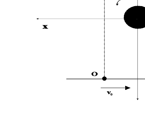
Figure 1: Configuration of the problem. The trajectory of the signals is assumed to be straight. A Cartesian coordinate system, centered on the spinning mass, is used. The source is at $y_{1}$, the observer $O$ is at $y_{2}$. The observer is moving with the velocity $v_{0}$. Two symmetric situations (at different times) are considered.

We now specialize our analysis to a weak field condition such as the one we find within the solar system. In this case Cartesian (i.e. rectangular) coordinates are often used. Assuming that the $z$ axis coincides with the direction of the angular momentum three-vector (1) becomes

$$ds^{2}=g_{tt}dt^{2}+g_{xx}dx^{2}+g_{yy}dy^{2}+g_{zz}dz^{2}+2g_{xt}dxdt+2g_{yt}dydt$$ (4)

The $g$’s now depend on $x$ and $y$.

The weak field hypothesis is commonly used to neglect the effect on the time of flight, of the bending of the trajectory due to the central mass [9]. This assumption, appropriately choosing the $x$ and $y$ axes, leads to a ray trajectory that is a straight line $x=b=const$; $b$ is of course the closest approach distance with respect to the spinning body. We must add the explicit form of the weak field metric elements

$$g_{yt} = G\frac{2Max}{c\left(x^{2}+y^{2}\right)^{\frac{3}{2}}}$$

$$g_{tt} = c^{2}-G\frac{2M}{\sqrt{x^{2}+y^{2}}}$$

$$g_{yy} = -1-G\frac{2M}{c^{2}\sqrt{x^{2}+y^{2}}}$$

Here $M$ is the mass of the central body, $J$ is its angular momentum, and $a=\frac{J}{Mc}$.

Under these conditions the time of flight of the electromagnetic signals becomes

$$t_{f}(y_{1},y_{2})=t_{0}+t_{M}+t_{J}$$ (5)

where (see [10] and [11])

$$t_{0} = \frac{y_{2}-y_{1}}{c}$$ (6)

$$t_{M} = \frac{2GM}{c^{3}}\ln\frac{y_{2}+\sqrt{b^{2}+y_{2}^{2}}}{y_{1}+\sqrt{b^{2}+y_{1}^{2}}}$$ (7)

$$t_{J} = \mp\frac{2GMa}{c^{3}b}\left[\frac{y_{2}}{\sqrt{b^{2}+y_{2}^{2}}}-\frac{y_{1}}{\sqrt{b^{2}+y_{1}^{2}}}\right]$$ (8)

The quantity $y_{1}$ is the $y$ coordinate of the source of the signals, $y_{2}$ is the $y$ coordinate of the receiver. The time $t_{0}$ is clearly the Newtonian time of flight; $t_{M}$ is the known gravitational time delay (Shapiro time delay), and $t_{J}$ is the correction to the time delay produced by the gravitomagnetic interaction with the angular momentum of the central body.
The double sign in $t_{J}$ means that gravitomagnetism shortens the time of flight on the left and lengthens it on the right.

4 Variable impact parameter

In general $y_{1}$ and $y_{2}$ will not be fixed and, consequently, the whole time delay will vary in time. Let us simplify the situation assuming that the source of the electromagnetic radiation is much more distant from the spinning body than the receiver. The source is then pointing out a fixed direction in space, just as a far astronomical source would do, and the time variation of $y_{2}$ in the reference frame of the central mass may easily be converted in a time variation of $b$ from the viewpoint of the observer (receiver).

If we limit the consideration to a situation around the occultation of the source by the central body, the source and the observer will be almost opposed with respect to the center, and the time dependence of $b$ on $t$ will be approximately linear. From an arbitrary (but not too big with respect to the radius of the central body) distance $b_{0}$, and considering the approach to the occultation, we can write

$$b\simeq b_{0}-v_{0}t$$ (9)

where $v_{0}$ is a positive velocity (apparent transverse velocity of the source in the sky).

If we add the condition that the time scale of the change of $b$ with time is much bigger than the period $T$ of the incoming electromagnetic wave, we can expect the period to slowly change, in one period time, by the amount

$$\delta T=\frac{dt_{f}}{db}\frac{db}{dt}T$$ (10)

Explicitly performing the differentiations and letting $y_{1}\rightarrow-\infty$

$$\frac{\delta T}{T} = -\frac{\delta\nu}{\nu}=\frac{2GM}{c^{2}}\frac{b^{2}+2\sqrt{b^{2}+y_{2}^{2}}y_{2}+2y_{2}^{2}}{b\sqrt{b^{2}+y_{2}^{2}}\left(y_{2}+\sqrt{b^{2}+y_{2}^{2}}\right)}\frac{v_{0}}{c}$$ (11)

$$\mp 2\left(y_{2}^{3}+2b^{2}y_{2}+\left(b^{2}+y_{2}^{2}\right)^{\frac{3}{2}}\right)GM\frac{a}{c^{2}b^{2}\left(b^{2}+y_{2}^{2}\right)^{\frac{3}{2}}}\frac{v_{0}}{c}$$

Now $\nu$ represents the frequency of the signals.

A further reasonable assumption is that $b<<y_{2}\sim R$, where $R$ is the distance of the observer from the central body. Under this assumption and posing $\mu=G\frac{M}{c^{2}}$ (11) can be simplified to

$$\frac{\delta\nu}{\nu}=\allowbreak 4\frac{\mu}{b}\frac{v_{0}}{c}-\frac{\mu b}{R^{2}}\allowbreak\frac{v_{0}}{c}\allowbreak\mp 4\frac{\mu a}{b^{2}}\frac{v_{0}}{c}$$ (12)

As it can be seen, there is an effective frequency shift, which is red during the approach. The last contribution has different signs on the opposite sides, thus leading to an asymmetry in the frequency shift too.

Possible asymmetries caused by the gravitomagnetic influence of the Sun on the propagation of electromagnetic signals were indeed studied by Davies [12], who proposed an experiment using a pair of sattelites orbiting the Sun. The idea was to measure the time of flight difference between a clockwise and a counter-clockwise trajectory of electromagnetic signals going from the Earth to one of the satellites, then to the other, then back. Our proposal is different in that we are considering effects on the frequency of the signals.

Another approach to the asymmetries due to the angular momentum of the Sun was considered by Bertotti and Giampieri[13]. There a complete analysis of the Doppler shift led to a result including the effect we have worked out. Here we propose a specific method to obtain the relevant observable.

5 Evidencing the asymmetry

Let us assume that the electromagnetic signal is a pure harmonic wave, whose proper frequency is $\nu_{0}$. At a given time, not far from the occultation, the received frequency will be $\nu_{0}+\delta\nu=\nu_{0}\left(1+\alpha_{1}\mp\alpha_{2}\right)$ where $\alpha_{1}$ is the symmetric part of the shift, and $\alpha_{2}$ is the antisymmetric one.

Suppose now to be able to record the received signal for a given time span, from the $b_{0}$ line of sight distance from the central body up to the occultation, then again from the reappearance on the other side up to a symmetric line of sight distance $b_{0}$. The second recorded signal can be reversed in time, then superposed to the one corresponding to the approach interval. In symbols all this amounts to generate a compounded beating signal:

$$\xi = \xi_{0}\left(\sin\left(2\pi\nu_{0}\left(1+\alpha_{1}-\alpha_{2}\right)t\right)+\sin\left(2\pi\nu_{0}\left(1+\alpha_{1}+\alpha_{2}\right)t\right)\right)$$

$$= 2\xi_{0}\cos\left(2\pi\nu_{0}\alpha_{2}t\right)\sin\left(2\pi\nu_{0}\left(1+\alpha_{1}\right)t\right)$$

Here $\xi_{0}$ is the constant amplitude of the original signal.

The resulting signal has a (slowly) time varying frequency

$$\nu_{1}=\nu_{0}\left(1+4\frac{\mu}{b}\frac{v_{0}}{c}-\frac{\mu b}{R^{2}}\allowbreak\frac{v_{0}}{c}\right)$$ (14)

and a modulated amplitude, whose modulation frequency is (again with a slow change in time)

$$\nu_{2}=4\nu_{0}\frac{\mu a}{b^{2}}\frac{v_{0}}{c}$$ (15)

6 Numerical estimates

To fix a few numbers, we can consider the situation in the solar system, with the Sun as the central spinning body, and an Earth bound observer. The source is a far away astronomical body (e.g. a pulsar). In this case the orders of magnitude are

$$\begin{array}[]{ccccc}\mu\sim 10^{3}\mathit{\ m}&a\sim 10^{3}\mathit{\ m}&b\sim 10^{9}\mathit{\ m}&R\sim 10^{11}\mathit{\ m}&v_{0}\sim 10^{4}\mathit{\ m/s}\end{array}$$

As a consequence we have

$$4\frac{\mu}{b}\frac{v_{0}}{c} \sim 10^{-10}$$

$$\frac{\mu b}{R^{2}}\allowbreak\frac{v_{0}}{c} \sim 10^{-14}$$ (16)

$$4\frac{\mu a}{b^{2}}\frac{v_{0}}{c} \sim 10^{-16}$$

The order of magnitude of the effective red shift is extremely small.

As for the beats, the smallness of their frequency implies a long time for significant changes in the amplitude of the resulting signal. The phase of the modulating wave is

$$\phi=8\pi\frac{\mu a}{b^{2}}\frac{v_{0}}{c}\nu_{0}t\sim 10^{-16}\nu_{0}t$$

which means that a full cycle happens when $\nu_{0}t\sim 10^{16}$. This condition requires a longer or shorter time according to the frequency of the signal: for optical frequencies 0.1 s would be enough; in the GHz range $10^{7}$s would be needed. Consider for comparison that the time required to move across the sky by one solar radius is, in these conditions, $\sim 10^{5}$ s; this means that a non-negligible effect on the amplitude could be seen using a signal in the GHz range and tracking it for $\sim 10^{5}$ s before and after the occultation of the source by the Sun.

7 Conclusion

We have evidenced a frequency effect connected with a varying time delay in the propagation of electromagnetic signals in the vicinity of a spinning massive body. The effect, if considered in solar system conditions is, as usual, very small, however not entirely negligible, at least when the trick proposed in the text is used, i.e. producing a beat between signals after and before the occultation. Of course many practical problems have to be considered and discussed to transform some principle formulae into an actual measurement. First of all one has to find the way to record the signals before and after an occultation event. Any recording device should contain a clock at a frequency higher than the one to be recorded; this seems to place a limit at a few GHz. Then the length of the record should not exceed the coherence time of the source, and this depends on the nature of the source. Furthermore there is also a problem with the amplitude and frequency stability of the signal. If the source is an actual clock on board a spacecraft, the formulae expressing the time delay are also geometrically more complicated, because of the not negligible motion of the source.

We can also envisage more favorable conditions. In case, for instance, we could find a pulsar orbiting a neutron star, the minimum impact parameter $b$ would be $\sim 10^{4}$ m. Keeping the same values for the rest, the asymmetric contribution to the frequency shift (last term in 12 and 16) would be $\sim 10^{-6}$, which is indeed easy to detect. For a typical frequency of the signal $10^{3}$ Hz the time needed to fully measure the beats we have described in sect. 5 would be $\sim 10^{3}$ s (20 minutes).

The conclusion we can draw at this point is that the method we propose seems promising for detecting gravitomagnetic effects on the propagation of electromagnetic signals, and for measuring the angular momenta of astronomical bodies.

References

- [1] Shapiro I.I., Phys. Rev. Lett., 13, (1964) 789
- [2] Shapiro I.I., Phys. Rev., 141, (1966) 1219
- [3] Einstein A. , The Meaning of Relativity, Princeton University Press, Princeton, N.J., 1950
- [4] Shapiro I.I. et al., Phys.Rev. Lett., 26, (1971) 1132
- [5] Anderson J.D. et al., Astrophys. J., 200, (1975) 221
- [6] Shapiro I. I., Reasenberg R. D. et al., J. Geophys. Res., 82, (1977) 4329
- [7] Reasenberg R. D., Shapiro I. I. et al., Astrophys. J. 234, (1979) L219
- [8] Ciufolini I., Ricci F., Class. Quantum Grav., 19, (2002) 3863
- [9] Straumann N., ’General Relativity and relativistic astrophysics’, Springer-Verlag (1988), Berlin and Heidelberg, pag. 184
- [10] Ohanian H.C., Ruffini R., Gravitation and Spacetime, W.W. Norton and Company, 1994
- [11] Ruggiero M.L., Tartaglia A., to be published in Nuovo Cimento B, Los Alamos Archives gr-qc/0207065
- [12] Davies R. W., Proceedings of the LVI school of physics Enrico Fermi, p. 405, ed. B. Bertotti, pub. Academic Press (1974), New York and London
- [13] Bertotti B., Giampieri G., Class. Quantum Grav., 9, (1992) 777