Testing a theory of gravity in celestial mechanics: a new method and
its first results for a scalar theory

Abstract

A new method of post-Newtonian approximation (PNA) for weak gravitational fields is presented together with its application to test an alternative, scalar theory of gravitation. The new method consists in defining a one-parameter family of systems, by applying a Newtonian similarity transformation to the initial data that defines the system of interest. This method is rigorous. Its difference with the standard PNA is emphasized. In particular, the new method predicts that the internal structure of the bodies does have an influence on the motion of the mass centers. The translational equations of motion obtained with this method in the scalar theory are adjusted in the solar system, and compared with an ephemeris based on the standard PNA of GR.

1 Introduction

One first expects from a theory of gravity that it should provide an accurate celestial mechanics. In other words, the theory should tell us how massive celestial bodies precisely move with respect to each other under the effect of the gravitational field produced by them all. Thus, Einstein’s general relativity (GR) won its first advantage over the older theory of Newton when it gave an explanation to Mercury’s residual advance in perihelion. In 1972, Weinberg stated about this explanation ([1], p. 198):“This is by far the most important experimental verification of general relativity.” It is hence extremely important for a theory of gravitation, not only that it produces accurate ephemerides, but even more that one is sure that it really produces those ephemerides, i.e., that the solution of the approximate equations used in the computation does approach accurately enough the relevant solution of the exact equations. The works of Fock [2] and Chandrasekhar [3] aimed at answering the latter question for GR. The later work on celestial mechanics in GR relies on essentially the same approximation scheme as these two works, which are equivalent in this regard. Yet in 1966, Synge, who did know Fock’s work (which is quoted in Ref. [4]) and most probably knew also that of Chandrasekhar, wrote [5]:“I am still waiting for a rational treatment of the dynamics of the solar system according to Einstein’s theory. In the very nature of the case, any argument must be of an approximate nature; an assessment of the error is a primary desideratum.” Comparing his successive sentences, we may infer that Synge was not satisfied with the approximation method used in the works [2, 3] nor with the one he himself proposed with coworkers [6, 4], and which was limited to stationary fields—this restriction is indeed inappropriate to describe the solar system in a realistic way.

The aim of this paper is to summarize the principles, the development and the numerical implementation of a new approximation method for celestial mechanics in relativistic theories of gravitation. This approximation method might have satisfied Synge, perhaps, because it is mathematically sound and general, and because it too predicts a salient result which he found in his work for GR [6, 4], namely the fact that, in such theories, the internal structure of a body does influence the gravitational field produced by it, hence also the motion of external bodies [9, 10]. The new method consists basically in associating a one-parameter family $(\mathrm{S}_{\lambda})$ of gravitating systems with the physically given system $\mathrm{S}$, by defining a family of initial conditions. It was initiated by Futamase & Schutz [7] for GR, with further mathematical developments given by Rendall [8]. However, Futamase & Schutz [7] assumed a very restrictive initial condition for the spatial metric. As to Rendall [8], he considered an a priori given one-parameter family of solutions of the field equations, without investigating the definition of a such family from the given system $\mathrm{S}$. Moreover, these two works were limited to the local equations and some of their mathematical properties. In particular, they did not provide equations of motion for the mass centers of a system of extended bodies, as one needs to compute an ephemeris. We came to the new method independently [11, 12], to test an alternative theory of gravitation based on just a scalar field [13, 14], and we did obtain such equations of motion [15, 9, 10]. That scalar theory gives the same predictions as GR for light rays [11]. Therefore, it is worth testing this theory further. Moreover, since that theory is much simpler than GR, it is easier to implement the new method for that theory, as well as to discuss the difference between the new method and the standard PNA.

2 General framework: the method of asymptotic expansions

As is well-known, an asymptotic expansion of a real function $\varphi$ of the real variable $\lambda$ in the neighborhood of some value $\Lambda$ is an expression

$$\varphi(\lambda)=a_{0}\psi_{0}(\lambda)+...+a_{n}\psi_{n}(\lambda)+R(\lambda),$$ (1)

the known functions $\psi_{0}$, …, $\psi_{n}$ being positive and belonging to a definite comparison set E, endowed with certain properties, and with $\psi_{0}\gg...\gg\psi_{n}\gg R$ as $\lambda\rightarrow\Lambda$ [16]. In physics, the relevant value is usually $\Lambda=0$, and one speaks of the “small parameter” $\lambda$. In particular, if the behaviour as $\lambda\rightarrow 0$ is regular enough, a Taylor expansion may apply, so that $\psi_{k}(\lambda)=\lambda^{k}(k=0,...,n)$. However, it may be that the Taylor expansion can be pushed only to some order $n=n_{\mathrm{max}}$, beyond which a more accurate expansion can be obtained only if one accepts to consider more general functions, e.g. ones involving a fractional exponent $k$. This remark is relevant to weak-field expansions in relativistic theories of gravitation.

Now consider a boundary-value problem defined for a given system of partial differential equations (PDE’s), and assume that a small parameter $\lambda$ can be defined for this problem, which means in fact that a family $(\mathrm{P}_{\lambda})$ of problems can be defined. The method of asymptotic expansions for this problem consists in trying to write each scalar component of the solution of $\mathrm{P}_{\lambda}$, say $\varphi_{i}^{(\lambda)}$ (where $i=1,...,m$ with $m$ the number of scalar unknowns involved in the system of PDE’s), as an asymptotic expansion in $\lambda$. That expansion is thus assumed valid at each given point $X\in\mathrm{D}$, where $\mathrm{D}$ is the relevant domain for the independent variables (space and time, say), which are collectively denoted by $X$. Actually this domain itself may well depend on $\lambda$, but, in order that one may write definite expansions (1) involving known functions $\psi_{k}(\lambda)$, it is preferable to absorb this dependence in a redefinition of the independent variables such that the expansions indeed apply to any given point $X$ in a domain independent of $\lambda$. If we look for a Taylor expansion, we write thus:

$$\forall X\in\mathrm{D},\quad\varphi_{i}^{(\lambda)}(X)=\varphi_{i0}(X)+...+\varphi_{in}(X)\lambda^{n}+R_{i}(X,\lambda),$$ (2)

with $R_{i}(X,\lambda)\ll\lambda^{n}$ as $\lambda\rightarrow 0$. The problem which is really of physical interest, $\mathrm{P}$, e.g. the initial-value problem for some (assumed) isolated self-gravitating system, is assumed to correspond to a given, small value $\lambda_{0}$ of the parameter. One of the difficulties of the method is definition of an adequate family $(\mathrm{P}_{\lambda})$, from the given problem $\mathrm{P}$. Once this has been done and once expansions as $\lambda\rightarrow 0$, and corresponding expanded equations, have been obtained for the family $(\mathrm{P}_{\lambda})$, they are then used for the finite value $\lambda_{0}$. This means that the error involved is the value for $\lambda_{0}$ of the unknown remainder $R_{i}(X,\lambda)$. In the case of a Taylor expansion, however, the remainder will usually be $O(\lambda^{n+1})$, and this uniformly with respect to $X\in\mathrm{D}$ (the relevant domain $\mathrm{D}$ being often compact). Although this is only an asymptotic error estimate, thus not a numerical one, it can be said that, if $\lambda^{n+1}$ is negligible with respect to the experimental accuracy, then the $n$-th order expansion (2) is very likely to be enough accurate for a meaningful experimental test. This seems to be the best that one can hope in the current state of the theory of PDE’s.

Why is it useful to write expansions at all? Mainly because the resulting equations are very greatly simplified: as it turns out, all non-linearities are reported in the equations of the order zero, and those are often much simpler than the starting equations. We emphasize two points:

i) It is indeed necessary to define a family of boundary-value problems (instead of contenting oneself with just that problem which one is interested in). This is in order that it just make sense to try expansions in $\lambda$: if we have defined a such family, we can then expand with respect to $\lambda$ each of the various coefficients that define the system of PDE’s, and we also can expand the boundary values. Only in that case can we derive expansions of the solution fields, and expanded equations for them, and then solve these equations using the expanded boundary conditions.

ii) One should indeed expand all independent unknown fields, $\varphi_{i}^{(\lambda)}$ for $i=1,...,m$ (and not just those which one likes to expand). For this allows one to write each equation as a sum of terms, each of a definite order in $\lambda$, this allowing in turn to separate the equations of the different orders: $k=0,...,n$—which is necessary, because an expansion like (2) means that a field $\varphi_{i}^{(\lambda)}$ is, after expansion, split into the $(n+1)$ fields $\varphi_{i0},...,\varphi_{in}$. Thus, if we write expansions for the $m$ independent unknown fields, using expansions with $(n+1)$ terms (e.g. Taylor expansions of order $n$), then we get each of the $m$ independent equations split into $(n+1)$ equations, so that we now have $m(n+1)$ equations for $m(n+1)$ unknowns. Whereas, if one expands only $p$ among the independent fields (with $p<m$), using expansions with $(n+1)$ equations, then one has (of course!) no reason to split the equations. But if one nevertheless would do so, then one would have too much equations (if $n\geq 1$): $m(n+1)$ equations for $p(n+1)+m-p$ unknowns.

The above-described method is merely the general formulation of a natural perturbation method for a system of PDE’s, and it is certainly not new. Of course there is a vast literature on perturbation methods (see e.g. Refs. 17–18 and references therein), and there are many common points between the different approaches. Yet we have not been able to find a description like the foregoing one, which applies very closely to what we actually did for the scalar theory of gravitation. Certainly also, the knowledge of PDE’s and of rigorous perturbation methods has considerably improved since the fifties. This may explain why the method developed for weak fields in GR by Fock [2] and Chandrasekhar [3] does not fulfil the requirements i) and ii) above—in fact it is based on formally taking $1/c^{2}$ as a small parameter (with $c$ the velocity of light), and in expanding the gravitational field, but not the matter fields, in powers of $1/c^{2}$.

3 Asymptotic post-Newtonian approximation of the scalar theory

It is the application of the foregoing method to the case of that “relativistic” theory of gravitation. In such theories, the relevant boundary-value problem is the initial-value problem. This is due to the hyperbolic character of the gravitational equation, in other words it comes from the fact that, in such theories, gravitation propagates with a finite velocity, usually equal to the velocity of light $c$ or close to $c$. This applies [12] to the scalar theory investigated by the author. Note, however, that the complete system of local equations is not closed, hence in particular cannot be qualified “hyperbolic”, until one has postulated a definite behaviour for matter, by assuming a constitutive equation giving the material energy-momentum tensor $\mathbf{T}$ in terms of some matter fields. For the sake of simplicity, we assume a perfect barotropic fluid, for which one has only the pressure $p$ and the (spatial) velocity $\mathbf{u}$ as independent matter fields.

Thus we consider a given, isolated gravitating system $\mathrm{S}$, made of $N$ separated bodies. That system is defined by the barotropic state equations in the different bodies, and by the initial data for the independent matter fields $p$ and $\mathbf{u}$, as well as for the scalar gravitational field $f$ and for its time derivative $\partial_{T}f$. (In GR, an initial data for the gravitational field is much more complicated, because the latter field is a tensor one, also because the Einstein equations are underdetermined, and above all because the initial conditions have to verify nonlinear constraint equations [21, 22].) The first task is to define a family $(\mathrm{S}_{\lambda})$ of gravitating systems, by defining a family of initial data and state equations. We want to describe weakly gravitating systems, for which Newton’s theory with its Euclidean space and absolute time must be an excellent approximation. For this to be true, the family $(\mathrm{S}_{\lambda})$ must satisfy two conditions as $\lambda\rightarrow 0$: i) the (physical, or “effective”) space-time metric $\boldsymbol{\gamma}$ must tend towards a flat metric $\boldsymbol{\gamma}^{0}$, and ii) all fields must become closer and closer to “corresponding” Newtonian fields. For the scalar theory, which is bimetric, the flat metric $\boldsymbol{\gamma}^{0}$ always coexists with the physical one $\boldsymbol{\gamma}$, and their local difference is an increasing function of $1-f$, which is non-negative [12]. Condition i) is hence easy to be made precise for the scalar theory: it means simply that the maximum value of the field $(1-f^{(\lambda)})$ must tend towards zero as $\lambda\rightarrow 0$. The parameter is

$$\lambda=\mathrm{Sup}_{\mathbf{x}\in\mathrm{M}}[1-f^{(\lambda)}(\mathbf{x},T=0)]/2.$$ (3)

where $\mathrm{M}$ is the “space” manifold, i.e. the set of the positions $\mathbf{x}$ in the preferred reference frame (PRF).

To make condition ii) precise, we use a crucial result [7, 12], namely the existence of an exact similarity transformation in Newton’s theory for barotropic fluids. Suppose we have the following fields: pressure $p^{(1)}$, density $\rho^{(1)}=F^{(1)}(p^{(1)})$, Newtonian potential $U_{N}^{(1)}$, and velocity $\mathbf{u}^{(1)}$, obeying the continuity equation, Poisson’s equation, and Euler’s equation. Then, for any $\lambda>0$, the fields $p^{(\lambda)}(\mathbf{x},T)=\lambda^{2}p^{(1)}(\mathbf{x},\sqrt{\lambda}\ T)$, $\rho^{(\lambda)}(\mathbf{x},T)=\lambda\rho^{(1)}(\mathbf{x},\sqrt{\lambda}\ T)$, $U_{N}^{(\lambda)}(\mathbf{x},T)=\lambda U_{N}^{(1)}(\mathbf{x},\sqrt{\lambda}\ T)$, and $\mathbf{u}^{(\lambda)}(\mathbf{x},T)=\sqrt{\lambda}\ \mathbf{u}^{(1)}(\mathbf{x},\sqrt{\lambda}\ T)$, also obey these equations—provided the state equation for system $\mathrm{S}_{\lambda}$ is $F^{(\lambda)}(p^{(\lambda)})=\lambda F^{(1)}(\lambda^{-2}p^{(\lambda)})$. This similarity transformation defines the weak-field limit in Newton’s theory itself: as $\lambda\rightarrow 0$, the potential and the density in the bodies decrease like $\lambda$ (while the bodies keep the same size), the (orbital) velocities decrease like $\sqrt{\lambda}$, and accordingly the time scale increases like $1/\sqrt{\lambda}$.

This exact similarity transformation does not extend to a “relativistic” theory like the scalar theory, simply because the equations are different. In particular, the metric changes as the gravitational field becomes stronger, and this changes the motion in a complex manner. Recall, however, that we merely seek initial conditions for the fields in the scalar theory. It is then obvious that, in order to precise condition ii), we simply have to apply the Newtonian similarity transformation to the initial fields. For the matter fields, this application is indeed immediate, because for a perfect fluid these are common to Newton’s theory and to a relativistic theory (via some slight modifications): pressure $p$, proper rest-mass density $\rho^{*}$ (instead of the invariant density of Newton’s theory), mass density of elastic energy $\Pi$, coordinate velocity $\mathbf{u}=d\mathbf{x}/dT$ (for the scalar theory, $T$ is the preferred time coordinate or “absolute time”, and $\mathbf{x}$ is the position in the preferred reference frame (PRF)). The mere difficulty is that, to apply the transformation, we must also associate a kind of “Newtonian potential” with the scalar gravitational field $f$. To do that, we assume in advance that a family $(\mathrm{S}_{\lambda})$ of systems has been built, which is such that the orders in $\lambda$ of the matter fields are the same, as $\lambda\rightarrow 0$, as in the Newtonian similarity transformation, and such that the field $f^{(\lambda)}$ admits an expansion of the form $f^{(\lambda)}=1+\phi\lambda^{k}+O(\lambda^{k+1})$. We find then that one must have $k=1$, i.e. the field $1-f^{(\lambda)}$ is like $\lambda$ as $\lambda\rightarrow 0$, thus like the potential in the Newtonian weak-field limit. It is hence natural to define that field, more precisely $V^{(\lambda)}=(c^{2}/2)(1-f^{(\lambda)})$, as the equivalent of the Newtonian potential $U_{N}^{(\lambda)}$; the coefficient is needed to ensure that $V^{(\lambda)}\sim U_{N}^{(\lambda)}$ as $\lambda\rightarrow 0$. Moreover, the local difference between the flat metric $\boldsymbol{\gamma}^{0}$ and the curved physical metric $\boldsymbol{\gamma}$ is an increasing function of $1-f^{(\lambda)}(\mathbf{x},T$).

In that way, we get the initial conditions for system $\mathrm{S}_{\lambda}$. Then we state powers expansions in $\lambda$ for the independent fields $f$, $p$, $\mathbf{u}$, and we deduce expansions for the other fields. The set of the obtained expansions and expanded equations is internally consistent, moreover it is consistent with the initial aim, in that the equations of the order 0 are indeed the “Euler-Newton” equations, i.e. the equations for a perfect fluid in Newton’s theory. The first PN corrections correspond to the equations of the order 1. The details can be found in Ref. 12 (see Ref. 15 for a synopsis and a few complementary points). Let us mention here some important points:

– We use a change of the mass and time units for system $\mathrm{S}_{\lambda}$, adopting $[\mathrm{M}]_{\lambda}=\lambda[\mathrm{M}]$ and $[\mathrm{T}]_{\lambda}=[\mathrm{T}]/\sqrt{\lambda}$ as the new units (where $[\mathrm{M}]$ and $[\mathrm{T}]$ are the starting units); then all fields are $\mathrm{ord}(\lambda^{0})$, and the small parameter $\lambda$ is proportional to $1/c^{2}$ (in fact $\lambda=(c_{0}/c)^{2}$, where $c_{0}$ is the velocity of light in the starting units). That $1/c^{2}$, not $1/c$, turns out to be the effective small parameter, is due to the fact that it is only $1/c^{2}$ that enters the equations. Thus, the derivation of the expansions and expanded equations is straightforward. In the standard PN scheme [2, 3], $1/c^{2}$ is formally considered as a small parameter, and the matter fields are not expanded.

– Recall, however, that such Taylor expansions in $\lambda$ (or $1/c^{2}$) cannot be expected to apply to an arbitrary order $n$ [see after Eq. (1)]. In GR, it has been shown by Rendall [8] that the attainable order $n$ depends on the gauge condition: with the classical “harmonic gauge”, even the second PN approximation ($n=2$) cannot be solved for a general spatially compact system of bodies—but a different gauge condition allows to reach the order $n=3$. This kind of problem cannot occur in the scalar theory, because there is no gauge condition. However, only the first PN approximation ($n=1$) has been studied in the scalar theory. If the matter sources are considered given (as was done in GR by Rendall [8]), then the PN gravitational field depends on integrals whose integrand is regular and vanishes outside the bodies [see Eqs. (24)–(26) below], so the first PN approximation is unproblematic.

– The equations of the order 1 are linear with respect to the fields of the order 1, so that the nonlinearities are confined to the zero-order (Euler-Newton) equations. The separation between the matter fields of the different orders, as well as the linearity in the PN fields, are characteristic of the asymptotic method, as contrasted with the standard PN scheme [2, 3]. It seems worth to illustrate the difference between the two approximations by exhibiting some simple equations.

4 Illustrating and commenting the difference between “standard” and “asymptotic” PNA’s

In the asymptotic PNA of the scalar theory, the rest-mass density in the PRF, $\rho_{\mathrm{exact}}$, is approximated as

$$\rho_{\mathrm{exact}}=\rho_{(1)}[1+O(\lambda^{2})],\qquad\rho_{(1)}\equiv\rho+\rho_{1}/c^{2},$$ (4)

and the like for the other fields, e.g. the velocity field $\mathbf{u}_{\mathrm{exact}}$. (For the zero-order, Newtonian fields, we shall omit the index 0 and shall thus keep the usual notation, while denoting henceforth the exact fields by the subscript “exact”.) The first-order (1PN) expansion of the time component of the local equations of motion for a perfect fluid is [12]

$$\partial_{T}\rho+\partial_{j}(\rho u^{j})=0,$$ (5)

$$\partial_{T}(w+\rho_{1})+\partial_{j}[(w+p+\rho_{1})u^{j}+\rho u_{1}^{j}]=-\rho\,\partial_{T}U,\qquad w\equiv\rho(\frac{\mathbf{u}^{2}}{2}+\Pi-U)$$ (6)

($U\equiv\mathrm{N.P.}[\rho]$ is the Newtonian potential associated with the 0-order mass density $\rho$). The 0-order spatial component of the local equations of motion is just the Newtonian equation of motion:

$$\partial_{T}(\rho u^{i})+\partial_{j}(\rho u^{i}u^{j})=\rho U_{,i}-p_{,i}.$$ (7)

Combining (7), the continuity equation (5), and the 0-order expansion of the isentropy equation:

$$d\Pi=-p\,d(1/\rho),$$ (8)

one gets in a standard way the Newtonian energy equation:

$$\partial_{T}w+\partial_{j}[(w+p)u^{j}]=-\rho\,\partial_{T}U.$$ (9)

Subtracting (9) from (6) gives us

$$\partial_{T}\rho_{1}+\partial_{j}(\rho_{1}u^{j}+\rho u_{1}^{j})=0,$$ (10)

which means that mass is conserved at the first PNA of the scalar theory.

In contrast, the standard 1PN expansion of the time component of the local equations of motion for a perfect fluid in GR consists ([3], Eqs. (1) and (64)) of Eq. (5), plus

$$\partial_{T}\sigma+\partial_{j}(\sigma u^{j})+\frac{1}{c^{2}}(\rho\partial_{T}U-\partial_{T}p)=0,\quad\sigma\equiv\rho[1+\frac{1}{c^{2}}(\mathbf{u}^{2}+2U+\Pi+\frac{p}{\rho})].$$ (11)

(Fock [2] gives only an integral form of the equations of motion.) In the equations (5) and (11) of the standard PNA of GR, however, $\rho$, $\mathbf{u}$ and $p$ are not defined except as exact fields ([3], Eqs. (4) and (5)), and, actually, they have to be considered as the second approximation of the exact fields—instead of being the zero-order expanded fields as in Eqs. (5) and (6) of the asymptotic PNA of the scalar theory. Thus, each of the matter fields is there only in one “exemplar” in the equations of the standard PNA. On the other hand, Chandrasekhar [3] does not regard Eqs. (5) and (11) as exact ones: rather, Eq. (5) is assumed valid if one neglects $O(1/c^{2})$ terms, and Eq. (11) is assumed valid if one neglects $O(1/c^{4})$ terms. Also note that, unlike our Eq. (6) of the asymptotic PNA, the PN equation (11) is not a “split” equation. Just the same remarks apply to the spatial components of the local equations of motion. As to the gravitational field, it is expanded in the standard PNA: at the first approximation, there is only the Newtonian potential $U$, whereas “PN potentials” $U_{i}$ and $\Phi$ are added in the second approximation. The Poisson equation applies to $U$:

$$\Delta U=-4\pi G\rho$$ (12)

(Eq. (3) in Ref. [3], Eq. (68.25) in Ref. [2]), and Poisson-like equations are derived for $U_{i}$ and $\Phi$.

In our opinion, the difficulty with the standard PNA is this: since the matter fields are not expanded, it follows that the equations of the first approximation are not exact ones resulting from a “splitting” (as it is the case in the asymptotic PNA). Instead, they result from a truncation and can, indeed, be valid only if one neglects $O(1/c^{2})$ terms (as Fock and Chandrasekhar noted). This point has been proved for the Poisson equation (12) in the scalar theory, in Ref. [12], Sect. 6.2. Thus, the “asymptotically correct” writing of Eq. (12) of the standard PNA is

$$\Delta U=-4\pi G\rho+O\left(\frac{1}{c^{2}}\right).$$ (13)

But this means that the field $U$ (the Newtonian potential) can be considered to be known only if one neglects $O(1/c^{2})$ terms. Now that field provides the main contribution to the acceleration, hence the equation of motion of the second approximation (Eq. (68) in Ref. 3) does of course include a term involving that field $U$ without an $1/c^{2}$ factor, namely the term $\rho\partial_{i}U$. This means that, at least if one restricts the discussion to the local equations, the second approximation does not provide a better approximation than up to $O(1/c^{2})$ terms not included—that is, it does not actually improve over the first approximation. Thus, if the first standard PNA is to really reach the $1/c^{2}$ level included, it must turn out that, at the later stage of the global equations of motion for the mass centers, and due to some mysterious integration effect, the low accuracy to which the Poisson equation can be considered valid has no effect any more. Moreover, as noted by Rendall [8], it may be dangerous to have PDE’s which are defined only up to unknown higher-order terms, which can change the type of the equation, e.g. from hyperbolic to elliptic. In conclusion, we prefer to stay with the “asymptotic” PNA summarized above, and to see where it leads.

5 Equations of motion for the mass centers: general PN equations

One may first ask whether there may be any satisfying definition of the mass center of a body in a “relativistic” theory of gravitation, given that: (i) in a theory accounting for the mass-energy equivalence, any form of material energy should be subjected to the action of the gravitational field; (ii) conversely, any form of material energy should contribute to the gravitational field; this means that the internal structure (through its energy distribution) and the internal motion (through the corresponding kinetic energy) are a priori expected to play a role [15]; for these two reasons, it is not obvious at all whether one single scalar mass-energy density can be used so as to define a single mass center, and which density this should be  [15]; (iii) in a generally-covariant theory like GR, a covariant definition should be found for the mass center—in other words, the motion of the latter should correspond to a single world-line in space-time, independently of which reference frame has been chosen [23]. The latter difficulty does not exist in the scalar theory, which has a preferred reference frame, but the two first ones subsist. Moreover, one has to ensure that the definition adopted will be astronomically relevant. With modern telescopes and other instruments, the major bodies of the solar system are, of course, very-well resolved as extended bodies, hence the astronomical position refers to an “optical center”. It seems to be a good approximation to admit that, once corrected from the “phase effects”, the latter corresponds to averaging the rest-mass density, because it is the body’s “matter”, in the usual sense, that does radiate electromagnetic energy. In any case, this density is certainly more relevant than any density involving gravitational energy, for the latter is distributed in the whole space. Therefore, we define the (exact) mass center by averaging the (exact) rest-mass density in the preferred frame, $\rho_{\mathrm{exact}}$ [15]. A theoretical argument also favours that density, and this is the fact that its PN approximation $\rho_{(1)}$, at least, obeys the usual continuity equation (see Eqs. (5) and (10)), thus without adding gravitational energy and its flux: this implies that the velocity of the mass center is itself the barycenter of the velocity—when the barycenter is defined with $\rho_{(1)}$ as the weight function [15].

Thus, we define the exact mass and mass center through the rest-mass density $\rho_{\mathrm{exact}}$ :

$$M_{a}^{\mathrm{exact}}\equiv\int_{\mathrm{D}_{a}}\rho_{\mathrm{exact}}dV,\qquad M_{a}^{\mathrm{exact}}\mathbf{a}_{\mathrm{exact}}\equiv\int_{\mathrm{D}_{a}}\rho_{\mathrm{exact}}\mathbf{x}dV$$ (14)

where $\mathrm{D}_{a}$ is the (time-dependent) domain occupied by body $(a)$ ($a=1,...,N$), in the PRF ($V$ is the Euclidean volume measure in the PRF). At the (first) PNA, the mass and the mass center are approximated by

$$M_{a}^{(1)}=M_{a}+M_{a}^{1}/c^{2},\qquad M_{a}\equiv\int_{\mathrm{D}_{a}}\rho dV,\qquad M_{a}^{1}\equiv\int_{\mathrm{D}_{a}}\rho_{1}dV,$$ (15)

$$M_{a}^{(1)}\mathbf{a}_{(1)}\equiv\int_{\mathrm{D}_{a}}\rho_{(1)}\mathbf{x}dV=M_{a}\mathbf{a}+M_{a}^{1}\mathbf{a}_{1}/c^{2},$$ (16)

with

$$M_{a}\mathbf{a}=\int_{\mathrm{D}_{a}}\rho\mathbf{x}dV,\qquad M_{a}^{1}\mathbf{a}_{1}=\int_{\mathrm{D}_{a}}\rho_{1}\mathbf{x}dV$$ (17)

Note that $M_{a}$ and $\mathbf{a}$ are the Newtonian mass and mass center. Using Eqs. (5) and (10), one shows that $M_{a}$ and $M_{a}^{1}$ are constant in time [15]. To get the PN equations of motion of the mass centers, one just integrates the spatial components of the PN local equations of motion inside the different bodies [15]. Due to the separation of the different orders in the local equations and to their linearity with respect to the PN fields, separate equations are also obtained for the mass centers, and the equation for PN corrections (order 1) is linear with respect to order-1 quantities. Specifically one finds [15]:

$$M_{a}\ddot{a}^{i}=\int_{\mathrm{D}_{a}}\rho U^{(a)}_{,i}dV$$ (18)

and

$$M_{a}^{1}\,\ddot{a}_{1}^{i}+\dot{I}^{ai}=J^{ai}+K^{ai},$$ (19)

with

$$I^{ai}\equiv\int_{\mathrm{D}_{a}}[p+\rho(\mathbf{u}^{2}/2+\Pi+U)]u^{i}dV,$$ (20)

$$J^{ai}\equiv\int_{\mathrm{D}_{a}}(\sigma_{1}U_{,i}+\rho A_{,i})dV,$$ (21)

$$K^{ai}\equiv\int_{\mathrm{D}_{a}}[2\mathsf{k}_{ij}p_{,j}+pU_{,i}-2U\rho U_{,i}-_{1}\Gamma_{jk}^{i}\rho u^{j}u^{k}-\rho u^{j}\partial_{T}\mathsf{k}_{ij}]dV.$$ (22)

In these equations, a point means (total) derivative with respect to the preferred time $T$; $\sigma_{1}$ is the PN correction to the active mass density, given by

$$\sigma_{1}=\rho_{1}+\rho(\mathbf{u}^{2}/2+\Pi+U);$$ (23)

$A$ is the PN gravitational potential, such that the PN expansion of the scalar field is

$$f^{(\lambda)}=1-2U/c^{2}-2A/c^{4}+O(\lambda^{3}),$$ (24)

and A is given by:

$$A=B+\partial^{2}W/\partial T^{2},$$ (25)

where $B\equiv\mathrm{N.P.}[\sigma_{1}]$ is the Newtonian potential associated with $\sigma_{1}$ and

$$W(\mathbf{X},T)\equiv\int GR\rho(\mathbf{x},T)dV(\mathbf{x})/2\qquad R\equiv\left|\mathbf{X-x}\right|$$ (26)

($G$ is the constant of gravitation); $2\mathsf{k}_{ij}/c^{2}$ and ${}_{1}\Gamma_{jk}^{i}/c^{2}$ are the components of the non-Euclidean part of the ”physical” space metric in the PRF and its associated connection, respectively, with

$$_{1}\Gamma_{jk}^{i}\equiv\mathsf{k}_{ij,k}+\mathsf{k}_{ik,j}-\mathsf{k}_{jk,i},\quad\mathsf{k}_{ij}\equiv U\mathsf{h}^{1}_{ij},\quad\mathsf{h}^{1}_{ij}\equiv\frac{U_{,i}U_{,j}}{U_{,k}U_{,k}};$$ (27)

{we use Cartesian coordinates for the Euclidean space metric $\boldsymbol{g}^{0}$, so that the PN physical space metric writes [12]

$$g^{(1)}_{ij}=\delta_{ij}+2\mathsf{k}_{ij}/c^{2};\}$$ (28)

and we use Fock’s decomposition [2] of any field $Z(\mathbf{x})$, integral of some density $\theta_{\mathbf{x}}$ vanishing outside the bodies, into “self ” and “external” parts $z_{a}(\mathbf{x})$ and $Z^{(a)}(\mathbf{x})$ :

$$Z(\mathbf{x})\equiv\int\theta_{\mathbf{x}}dV=z_{a}(\mathbf{x})+Z^{(a)}(\mathbf{x}),\quad z_{a}(\mathbf{x})\equiv\int_{\mathrm{D}_{a}}\theta_{\mathbf{x}}dV,Z^{(a)}(\mathbf{x})\equiv\sum_{b\neq a}\int_{\mathrm{D}_{b}}\theta_{\mathbf{x}}dV.$$ (29)

The zero-order equation, Eq. (18), is just the Newtonian translational equation of motion.

6 Equations of motion for the mass centers: relevant simplifications

Equation (19) for the PN corrections to the motion is not tractable. To make it explicit, we account for two simplifications that do occur for the major bodies of the solar system, namely: (i) the good separation between bodies (this occurs probably also for many other systems); (ii) the fact that the bodies are nearly spherical (this occurs almost certainly also for all other systems, if one considers individual bodies with large-enough mass).

Point (i) is defined by introducing the separation parameter [9]

$$\eta_{0}\equiv\max_{a\neq b}(r_{b}/\left|\mathbf{a-b}\right|),\qquad r_{b}\equiv\frac{1}{2}\mathrm{Sup}_{\mathbf{x},\mathbf{y}\in\mathrm{D}_{b}}\left|\mathbf{x-y}\right|,$$ (30)

and by assuming that it is small for the system of physical interest. (The zero-order positions of the mass centers are used, since the PN corrections to these positions are very small, hence would lead to nearly the same value for $\eta_{0}$.) In order to exploit this small parameter, we introduce again a (conceptual) family of gravitational systems, by defining initial conditions for them [10]. Thus, remembering the weak-field parameter $\lambda$, we actually would have a two-parameters family of systems. However, the local 1PN equations of the asymptotic method—thus the set of the first-order expansions, like (4), the set of the expanded equations, like (5) and (10), and the set of the expanded boundary conditions, derived in Refs. 12 and 15—are mathematically self-consistent, in that they make a closed system of equations. (They are not physically self-consistent yet, since they do not ensure by themselves that the weak-field/low-velocity assumptions are satisfied and remain so in time.) Hence we may content ourselves with deducing a one-parameter family $(\mathrm{S}^{\prime}_{\eta})$ of well-separated “PN systems” from the data of the given PN system $\mathrm{S}^{\prime}$, the latter being itself deduced from the given system $\mathrm{S}$ by substituting the 1PN equations for the exact ones. (Actually the local PN equations of the asymptotic method are exact, but they define merely a part of the exact fields [12].) The PN gravitational fields: $U=\mathrm{N.P.}[\rho]$, $B=\mathrm{N.P.}[\sigma_{1}]$, and $W$, depend merely on the PN matter fields [Eqs. 24–26]. Hence we just have to define the initial conditions for the PN matter fields. Moreover, the latter conditions turn out to be determined by the initial zero-order matter fields $p(T=0)$, or equivalently $\rho(T=0)$, and $\mathbf{u}(T=0)$ [12]. To define $\rho(T=0)$ in $\mathrm{S}^{\prime}_{\eta}$, we set

$$\mathbf{a}^{\eta}(T=0)=\mathbf{a}(T=0)\eta_{0}/\eta,$$ (31)

$$\rho^{\eta}(\mathbf{x},T=0)=\rho(\mathbf{a+y},T=0)\quad\mathrm{if}\quad\mathbf{x}=\mathbf{a}^{\eta}+\mathbf{y}\quad\mathrm{with}\quad\mathbf{a+y}\in\mathrm{D}_{a}.$$ (32)

Equation (32) defines $\rho^{\eta}$ so that the density inside the bodies is independent of $\eta$ [setting $\rho^{\eta}(\mathbf{x},T=0)=0$ if $\mathbf{x}$ does not have the form above for some $a=1,...,N$]. In other words, the bodies themselves do not depend on the separation parameter $\eta$. Equation (31) ensures that, at least near $T=0$, the separation distances between bodies are of order $\eta^{-1}$:

$$\left|\mathbf{a}^{\eta}-\mathbf{b}^{\eta}\right|=\mathrm{ord}(\eta^{-1}).$$ (33)

To define the velocity $\mathbf{u}^{\eta}(T=0)$, we use the auxiliary assumption that each body undergoes a rigid motion at the Newtonian approximation [2]:

$$u^{i}=\dot{a}^{i}+\Omega^{(a)}_{ji}(x^{j}-a^{j}),\,\mathrm{or}\,\mathbf{u}=\dot{\mathbf{a}}+\boldsymbol{\omega}_{a}\wedge(\mathbf{x-a})\,\mathrm{for}\,\mathbf{x}\in\mathrm{D}_{a},\,\Omega^{(a)}_{ji}+\Omega^{(a)}_{ij}=0.$$ (34)

Of course, this is only approximately true (e.g. due to the tidal influence of the other bodies), but we use this assumption merely to calculate the PN corrections. Since the latter ones are very small, it certainly implies only an extremely small error in the solar system. Anyhow, we can assume that (34) is exact at the initial time. From the Newtonian estimate $\dot{\mathbf{a}}^{2}\approx U^{(a)}(\mathbf{a})$ , valid in the reference frame of the global mass center, and from (33), we expect that, at any time,

$$(\dot{a}^{i})^{\eta}=\mathrm{ord}(\eta^{1/2}).$$ (35)

We assume that this is true if we define the initial translation velocities of system $\mathrm{S}^{\eta}$ as

$$(\dot{a}^{i})^{\eta}(T=0)=(\eta/\eta_{0})^{1/2}\dot{a}^{i}(T=0).$$ (36)

As to the self-rotation velocities, in the solar system they have at most the same magnitude, in linear values, as the translation velocities, and our numerical calculations show that the PN corrections containing quadratic terms in $\Omega^{(a)}_{ji}$, included in the first version of the explicit translational equations [9], are negligibly small in the solar system. To avoid such terms in the expansions, it turns out to be sufficient that

$$(\Omega^{(a)}_{ji})^{\eta}\ll\eta^{1/2},$$ (37)

hence we set, for some small number $\varepsilon>0$,

$$(\Omega^{(a)}_{ji})^{\eta}(T=0)=(\eta/\eta_{0})^{\varepsilon+1/2}\,\Omega^{(a)}_{ji}(T=0),$$ (38)

and we assume that this ensures that (37) is true at any time.

Point (ii) is defined simply by assuming, merely at the stage of calculating the PN corrections, that the zero-order rest-mass density $\rho$ is spherically symmetric for each body:

$$\forall\mathbf{x}\in\mathrm{D}_{a},\,\rho(\mathbf{x})=\rho_{a}(r),\quad r\equiv\left|\mathbf{x-a}\right|\quad(a=1,...,N).$$ (39)

The sphericity of the field $\rho$ implies also that of the pressure field $p$ and the Newtonian self-potential $u_{a}$. By using this and point (i), i.e. Eqs. (33), (35) and (37), we get after rather involved calculations [9, 10]:

$$\frac{d\mathbf{u}_{1a}}{dT} = o(\eta^{3})+\left[\left(\frac{\tau_{a}}{M_{a}}-\frac{5}{6}\right)\mathbf{u}_{a}^{2}-\frac{5}{3}U^{(a)}(\mathbf{x}_{a})-\frac{17\varepsilon_{a}+6T_{a}}{3M_{a}}\right]\nabla U^{(a)}(\mathbf{x}_{a})$$ (40)

$$-\left[\left(\frac{\tau_{a}}{M_{a}}+2\right)\mathbf{u}_{a}\mathbf{.}\nabla U^{(a)}(\mathbf{x}_{a})\right]\mathbf{u}_{a}+\left[2\frac{\varepsilon_{a}}{M_{a}}+U^{(a)}(\mathbf{x}_{a})\right]\boldsymbol{\omega}_{a}\wedge\mathbf{u}_{a}$$

$$+G\sum_{b\neq a}\left\langle\frac{M_{b}}{2r_{ab}}\left[\left(\mathbf{n}_{ab}\mathbf{.}\dot{\mathbf{u}}_{b}\right)\mathbf{n}_{ab}-\dot{\mathbf{u}}_{b}\right]\right.$$

$$+\frac{1}{r_{ab}^{2}}\left\{-\alpha^{\prime}_{ab}\mathbf{n}_{ab}+\frac{M_{b}}{2}\left[\left(3(\mathbf{n}_{ab}\mathbf{.}\mathbf{u}_{b})^{2}-\mathbf{u}_{b}^{2}\right)\mathbf{n}_{ab}-\left(\mathbf{n}_{ab}\mathbf{.}\mathbf{u}_{b}\right)\left(2\mathbf{u}_{b}+\frac{8}{3}\mathbf{u}_{a}\right)\right]\right\}$$

$$+\left.\frac{M_{b}}{r_{ab}^{3}}\left[\mathbf{x}_{1b}\mathbf{-}\mathbf{x}_{1a}+3\left((\mathbf{x}_{1a}\mathbf{-}\mathbf{x}_{1b})\mathbf{.}\mathbf{n}_{ab}\right)\mathbf{n}_{ab}\right]\right\rangle,$$

with $r_{ab}\equiv\left|\mathbf{x}_{a}-\mathbf{x}_{b}\right|$, $\mathbf{n}_{ab}\equiv(\mathbf{x}_{a}-\mathbf{x}_{b})/r_{ab}$, and

$$\alpha^{\prime}_{ab}\equiv M_{b}\left(\frac{\mathbf{u}_{a}^{2}+\mathbf{u}_{b}^{2}}{2}+U^{(a)}(\mathbf{x}_{a})+U^{(b)}(\mathbf{x}_{b})+\frac{11\varepsilon_{a}+8T_{a}}{3M_{a}}\right)+M_{b}^{1}+\frac{11}{3}\varepsilon_{b}+\frac{8}{3}T_{b},$$ (41)

and where, as a preparation for the application, the notation for the PN positions and velocities of the mass centers has been changed, as compared with (16) and (17):

$$\mathbf{x}_{a}\equiv\mathbf{a},\quad\mathbf{x}_{1a}\equiv c^{2}(\mathbf{a}_{(1)}-\mathbf{a}),\qquad\mathbf{x}_{(1)a}\equiv\mathbf{a}_{(1)}=\mathbf{x}_{a}+\mathbf{x}_{1a}/c^{2}$$ (42)

$$\mathbf{u}_{a}\equiv\dot{\mathbf{a}},\quad\mathbf{u}_{1a}\equiv c^{2}(\dot{\mathbf{a}}_{(1)}-\dot{\mathbf{a}})=\dot{\mathbf{x}}_{1a},\quad\mathbf{u}_{(1)a}\equiv\dot{\mathbf{a}}_{(1)}=\mathbf{u}_{a}+\mathbf{u}_{1a}/c^{2}$$ (43)

Note that terms of order up to and including $\eta^{3}$ have been consistently retained in Eq. (40) [10]. In the first version of the explicit translational equations of motion [9], this could not be done due to the lack of an asymptotic framework for the separation parameter $\eta$, and this resulted in a large difference with observational data. In addition to the self-rotational energy:

$$T_{a}\equiv\Omega^{(a)}_{ik}\Omega^{(a)}_{jk}I^{(a)}_{ij}/2,\qquad I^{(a)}_{ij}\equiv\int_{D_{a}}\rho(x^{i}-a^{i})(x^{j}-a^{j})dV,$$ (44)

two structure-dependent parameters appear in (40):

$$\varepsilon_{a}\equiv\int_{D_{a}}\rho u_{a}dV/2,$$ (45)

$$\tau_{a}\equiv\frac{1}{3G}\int_{0}^{r_{a}}u_{a}\left\{\frac{4r\mu_{a}^{\prime}}{\mu_{a}(r)}-\left[\frac{r\mu_{a}^{\prime}}{\mu_{a}(r)}\right]^{2}\right\}dr,\qquad\mu_{a}(r)\equiv 4\pi\int_{0}^{r}\rho_{a}(s)s^{2}ds.$$ (46)

No such structure parameter does enter in the PN equations that have been used in celestial-mechanical tests of GR, namely the Lorentz-Droste-Einstein-Infeld-Hoffmann (LDEIH) equations, which are based on the standard PNA. However, as already noted by Synge and coworkers, one should expect that the internal structure of the bodies does influence the motion.

7 Numerical implementation. Comparison with an ephemeris based on the standard PNA of GR

In order to use the translational equations of motion (18) and (40), so as to check the scalar theory, we have to know the values of the independent parameters that enter these equations. These are: the zero-order masses $M_{a}$ of the bodies (here the major bodies of the solar system) and their parameters $T_{a}$, $\varepsilon_{a}$ and $\tau_{a}$; the initial conditions of their motion; and the constant velocity $\mathbf{V}$ of the global zero-order mass center of the solar system, with respect to the preferred frame E [9]. (Of course there is no parameter like $\mathbf{V}$ in conventional theories.) These unknown parameters depend on the theory. They have to be determined by optimizing the agreement between predictions and observations [9]. In particular, one may expect that the optimal values of the zero-order parameters should differ from their values in pure Newtonian theory by first-order (second-approximation) quantities, this fact alone giving corrections of the same magnitude as the 1PN corrections [9]. However, since the parameters $T_{a}$, $\varepsilon_{a}$ and $\tau_{a}$ play a role only in the PN corrections, such first-order corrections on their values would make only second-order differences, hence negligible ones, in the final results. Therefore, we calculate these parameters from the standard rotation velocities and density profiles of the corresponding bodies [24, 25].

Then our adjustment algorithm loops on the numerical solution of the translational equations of motion in order to optimize the remaining parameters, i.e., the zero-order masses $M_{a}$, the initial conditions, and the velocity $\mathbf{V}$. The algorithm has been tested [26] by investigating in which measure one may reproduce (over one century) the predictions of the DE403 ephemeris [27], by using purely Newtonian equations of motion. (The DE403 ephemeris is based on LDEIH-type equations of motion [28], thus it is based on the standard PNA of GR.) Our algorithm has also been applied to adjust a less simplified model, in which the PN corrections in the Schwarzschild field of the Sun are also considered, and to compare this model with DE406 [29] over 60 centuries [30]. It has thus been found that the difference between a calculation based on these “Schwarzschild-corrected” Newtonian equations, limited to the Sun and the nine major planets, and the DE406 ephemeris of the JPL, based on LDEIH-type equations and including the Moon and asteroids, is very small. Over the last century, for instance, the longitude difference for Mercury is $0.03^{\prime\prime}$ [30]. The VSOP82 ephemeris [31] is also based on “Schwarzschild-corrected” Newtonian equations, but it uses more accurate (semi-analytical) algorithms than ours; also, for the comparison with the JPL ephemerides, it seems that it takes Schwarzschild’s metric in “isotropic” form, rather than in the standard form in which we took it. The VSOP82 ephemeris leads to even smaller differences with an ephemeris based on LDEIH-type equations (e.g. $0.001^{\prime\prime}$ over 1891-2000 for the longitude of Mercury). Now the scalar theory does predict Schwarzschild’s motion for test particles in the field of one spherical body, if the latter is at rest in the preferred frame ($\mathbf{V}=0$). Hence, if we take for PN corrections in our theory those that are obtained by considering the planets as test particles in the field of the spherical Sun, and if we include $\mathbf{V}$ in the free parameters, then we can obtain only a smaller difference with the LDEIH-type equations than the difference between the latter and the “Schwarzschild-corrected” Newtonian equations. But, in our opinion, the correct equations of motion are those got with the asymptotic PNA. Therefore, we have implemented the equations (18) and (40) in our adjustment algorithm.

To do that, we had first to solve a numerical shortcoming of the asymptotic method, namely the fact that the mass center of a body, or the test particle, is followed on its trajectory by two different positions: the zero-order position $\mathbf{x}_{0}$ and the 1PN position, $\mathbf{x}_{(1)}\equiv\mathbf{x}_{0}+\mathbf{x}_{1}/c^{2}$, which drift from one another as the time goes. By investigating in detail the case of a test particle in a Schwarzschild field, it has been found that this leads to an error increase in $(T-T_{0})^{2}$, and that it may be cured by “reinitializing”, i.e., by substituting $T_{0}+\delta T$, then $T_{0}+2\delta T$, etc., with $\left|\delta T\right|$ sufficiently small, for the initial time $T_{0}$ in the differential system that governs the motion of the mass centers [32]. Moreover, since the equation for PN corrections (40) is valid only in the preferred reference frame E, we use a Lorentz transform to go from E to the frame $\mathrm{E}_{\mathbf{V}}$ bound with the zero-order global barycenter, and vice-versa. This transform, as well as the inverse transform, is determined by the free vector $\mathbf{V}$. Thus, the adjustment process of the translational equations on observational data provides us eventually with the value of $\mathbf{V}$ that minimizes the residual with the set of observations. However, the “observational data” are currently taken from an ephemeris based on GR, specifically here we took from DE403 a set of heliocentric positions of the eight major planets (Pluto omitted), between 1956 and 2000.

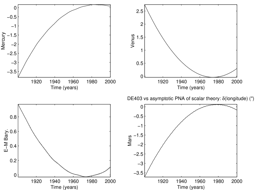
Figure 1: Longitude differences (arc seconds) for planets Mercury to March, either as taken from the DE403 ephemeris of the Jet Propulsion Laboratory, or as obtained (after adjustment) by numerical integration of the equations of motion in the asymptotic post-Newtonian approximation of the investigated scalar theory.

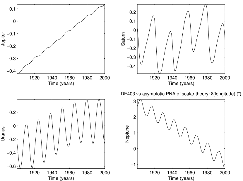
Figure 2: Longitude differences (arc seconds) for planets Jupiter to Neptune, either as taken from the DE403 ephemeris of the Jet Propulsion Laboratory, or as obtained (after adjustment) by numerical integration of the equations of motion in the asymptotic post-Newtonian approximation of the investigated scalar theory.

With these input data, themselves a fitting of observations by the LDEIH equations of GR, the magnitude of the optimal vector is $\left|\mathbf{V}\right|\approx 3\mathrm{km/s}$, which is significant. The difference between DE403 and our thus-adjusted equations of motion is shown on figures 1 and 2. The self-rotation of all nine bodies is neglected, i.e., all $\boldsymbol{\omega}_{a}$ ’s are assumed $\mathbf{0}$ in (34). We show only the difference in longitudes, because it dominates over the other errors. It can be seen that, for most planets, the difference is very small (a few times $0.1^{\prime\prime}$) over the fitting interval, but it increases quickly with time for the inner planets (Mercury, Venus, the Earth-Moon Barycenter (EMB), and Mars). We do not know yet whether this comes only from the different models or partly also from numerical reasons: due to the necessity of reinitializing very often (every two days here—we mean the ephemeris time, not the computer time), the calculations are long. It has already been checked that an increase of the accuracy in the ODE-solver brings negligible changes to the present Figure showing the differences between DE403 and the asymptotic PNA of the scalar theory. Anyhow, the differences are still quite small, e.g. $3.8^{\prime\prime}$ for Mercury after the last century, to be compared with the relativistic perihelion advance of $43^{\prime\prime}$, and with the accuracy of the current ephemerides, considered to be $0.1^{\prime\prime}$ for Mercury [33],p. 228. For the influence of the Moon on the motion of the EMB, we use a semi-analytical correction formula [34], which we adapted in an approximate way from the “1950 ecliptic” to the “J2000” reference.

8 Conclusion

The usual method of asymptotic expansions, as defined in Sect. 2, is indeed of usual utilization in most domains where partial differential equations occur, but it contrasts with the standard (Fock-Chandrasekhar) method of post-Newtonian approximation (PNA) for weak gravitational fields. In the latter method, no one-parameter family of similar problems is introduced, so that the meaning of the approximation is not very clear. Indeed $1/c^{2}$ is formally considered as a small parameter, and the matter fields are not expanded. We applied the usual method of asymptotic expansions to weak gravitational fields in our scalar theory, and we call the result the asymptotic PNA. A similar method has been proposed in GR by Synge and coworkers [6, 4] for stationary gravitational fields, and has been initiated in a more general case, but not fully developed, by Futamase & Schutz [7]. In our opinion, the asymptotic PNA is very solid mathematically. Within the asymptotic PNA, $1/c^{2}$ turns out to be (proportional to) the small parameter $\lambda$, but this is true in specific units, depending on $\lambda$. The asymptotic PNA leads to definitely different equations, as compared with the standard PNA. In particular, the former method predicts that the internal structure of the bodies, and their internal motion, has a definite influence on the motion of the mass centers of a self-gravitating system of bodies.

This has been checked numerically in the solar system for the scalar theory. The standard PNA should probably lead to the same result in the scalar theory as in GR, namely it should lead to the conclusion that, in the solar system, the post-Newtonian effects may be calculated simply by adding to the Newtonian motion the PN corrections obtained in considering all planets as test particles in the field of the isolated Sun. If the latter approximation is used, the results of our scalar theory are nearly indistinguishable from those of GR. In contrast, if the equations of the asymptotic PNA are used, then the predicted motion apparently cannot fit a standard ephemeris (i.e. an ephemeris based on the standard PNA of GR) within what is currently believed to be the observational accuracy.

It seems that the influence of the internal structure of the bodies and the difference with the DE403 ephemeris are much more the result of changing the approximation method, than that of changing the theory. Indeed, the exact local equations of motion for a perfect fluid in the scalar theory are very similar to those in GR, and the general metric of the theory is a “Schwarzschild-like” metric. In other words, the author considers it likely that a similar departure from a standard ephemeris would be left, if one compared it with a calculation based on an asymptotic PNA of GR. However, this could be proved only by building a general asymptotic scheme in GR. This would be difficult, due to the fact that in GR the initial conditions cannot be imposed freely.

Coming back to the scalar theory, there is still a possibility to improve the fitting, mainly by re-adjusting the masses (this could not be done here, except for those of the Sun and Jupiter, because the masses are sensible parameters whose values have to be separately optimized before possibly optimizing them globally), perhaps also by improving the numerical accuracy. It is also very important to adjust the equations, not on an ephemeris (because this is already a fitting of observations by some other equations), but directly on observations. Indeed some correction factors of observational data are taken as free parameters in the adjustment of an ephemeris, hence the observations are not completely independent of the gravitational model. Finally, it should be noted that the (best-fitting) value of the absolute velocity $\mathbf{V}$ of the mass center of the solar system has been found to be ca. 3 km/s with the present model (self-rotation neglected, adjustment on a standard ephemeris), and this already is not negligible. Due to these simplifications, and due to the fact that the solar system was assumed isolated here, this present best-fitting value of $\mathbf{V}$ is not even an approximation to the correct one: it justs tells an idea about the order of magnitude of $\mathbf{V}$. That this is not negligible, might incline one to think that the preferred-frame character of the theory is not redhibitory.

References

- [1] S. Weinberg, Gravitation and Cosmology (J. Wiley & Sons, New York, 1972).
- [2] V. A. Fock, The Theory of Space, Time and Gravitation (1st English edn., Pergamon, Oxford, 1959). (Russian original edn.: Teoriya Prostranstva, Vremeni i Tyagotenie, Gos. Izd. Tekhn.-Teoret. Liter., Moskva, 1955.)
- [3] S. Chandrasekhar, Astrophys. J. 142, 1488–1512 (1965).
- [4] P. S. Florides and J. L. Synge, Proc. Roy. Soc. London A 270, 467–492 (1962).
- [5] J. L. Synge, in Perspectives in Geometry and Relativity – Essays in Honor of Hlavaty, edited by B. Hoffmann (Indiana University Press, Bloomington and London, 1966), pp. 7–15.
- [6] A. Das, P. S. Florides and J. L. Synge, Proc. Roy. Soc. London A 263, 451–472 (1961).
- [7] T. Futamase and B. F. Schutz, Phys. Rev. D 28, 2363–2372 (1983).
- [8] A. D. Rendall, Proc. Roy. Soc. London A 438, 341–360 (1992).
- [9] M. Arminjon, Roman. J. Phys. 45, 659–678 (2000), astro-ph/0006093.
- [10] M. Arminjon, “Equations of motion of the mass centers in a scalar theory of gravitation: Expansion in the separation parameter”, submitted, gr-qc/0202029.
- [11] M. Arminjon, Rev. Roumaine Sci. Tech. – Méc. Appl. 43, 135–153 (1998), gr-qc/9912041.
- [12] M. Arminjon, Roman. J. Phys. 45, 389–414 (2000), gr-qc/0003066.
-
[13]
M. Arminjon, Rev. Roumaine Sci. Tech. – Méc. Appl. 42, 27–57 (1997). Online at
http://geo.hmg.inpg.fr/arminjon/pub_list.html#A18. -
[14]
M. Arminjon, Arch. Mech. 48, 25–52
(1996). Online at
http://geo.hmg.inpg.fr/arminjon/pub_list.html#A15 - [15] M. Arminjon, Roman. J. Phys. 45, 645–658 (2000), astro-ph/0006093.
- [16] J. Dieudonné, Calcul Infinitésimal (Hermann, Paris, 1968), chapter 3.
- [17] J. Kevorkian and J. D. Cole, Perturbation Methods in Applied Mathematics (Springer, New York Heidelberg - Berlin, 1981).
- [18] J. Awrejcewicz, I. V. Andrianov and L. I. Manevitch, Asymptotic Approaches In Nonlinear Dynamics (Springer, Berlin - Heidelberg - New York, 1998).
- [19] A. A. Logunov, Yu. M. Loskutov and M. A. Mestvirishvili, Sov. Physics Uspekhi 31, 581–596 (1988). (Usp. Fiz. Nauk 155, 369–396 (1988).)
- [20] A. Logunov and M. Mestvirishvili, The Relativistic Theory of Gravitation (Mir, Moscow, 1989). (Russian original edn.: Osnovy Relyativistskoi Teorii Gravitatsii, Izd. Mosk. Univ., Moskva, 1986.)
- [21] H. Stephani, General Relativity (Cambridge Univ. Press, Cambridge, 1982), pp. 152-161.
-
[22]
A. D. Rendall, Living Reviews in Relativity 3 (2000),
1, article on the web at
http://www.livingreviews.org/Articles/Volume3/2000-1rendall. - [23] R. Tucker, private communication at the 2nd British Meeting on Gravitation (BritGravII), June 2002.
- [24] P. Bakouline, E. Kononovitch and V. I . Moroz, Astronomie Générale (Mir, Moscow, 1975), pp. 102-105. (Russian 3rd edn.: Kurs obshcheii astronomii, Izd. Nauka, Moskva, 1973.)
- [25] J. S. Lewis, Physics and Chemistry in the Solar System (Academic Press, San Diego, 1995), pp. 138, 399 and 470.
- [26] M. Arminjon, “A numerical solution of the inverse problem in classical celestial mechanics, with application to Mercury’s motion”, to appear in Meccanica, 2003, astro-ph/0105217.
- [27] E. M. Standish, X. X. Newhall, J. G. Williams and W. M. Folkner, Jet Prop. Lab. Interoffice Memo. 314.10–127 (1995).
- [28] X. X. Newhall, E. M. Standish and J. G. Williams, Astron. & Astrophys. 125, 150–167 (1983).
- [29] E. M . Standish, Jet Prop. Lab. Interoffice Memo. 312.F–98–048 (1998).
- [30] M. Arminjon, Astron. & Astrophys. 383, 729–737 (2002), astro-ph/0112266.
- [31] P. Bretagnon, Astron. & Astrophys. 114, 278–288 (1982).
- [32] M. Arminjon, Nuovo Cimento B 116, 1277–1290 (2001), gr-qc/0106087.
- [33] J.-L. Simon, M. Chapront-Touzé, B. Morando and W. Thuillot (Eds.) Introduction aux Ephémérides Astronomiques (Bureau des Longitudes) (EDP Sciences, Paris, 1998).
- [34] P. Bretagnon, Astron. & Astrophys. 84, 329–341 (1980).
-
[35]
M. Arminjon, in Fifth Conf. “Physical Interpretations of
Relativity Theory”, Supplementary Papers (M.C. Duffy, ed.,
University of Sunderland/Brit. Soc. Philos. Sci., 1998), pp.
1–27. Online at
http://geo.hmg.inpg.fr/arminjon/pub_list.html#B13