Physics and Initial Data for Multiple Black Hole Spacetimes

Abstract

An orbiting black hole binary will generate strong gravitational radiation signatures, making these binaries important candidates for detection in gravitational wave observatories. The gravitational radiation is characterized by the orbital parameters, including the frequency and separation at the inner-most stable circular orbit (ISCO). One approach to estimating these parameters relies on a sequence of initial data slices that attempt to capture the physics of the inspiral. Using calculations of the binding energy, several authors have estimated the ISCO parameters using initial data constructed with various algorithms. In this paper we examine this problem using conformally Kerr-Schild initial data. We present convergence results for our initial data solutions, and give data from numerical solutions of the constraint equations representing a range of physical configurations. In a first attempt to understand the physical content of the initial data, we find that the Newtonian binding energy is contained in the superposed Kerr-Schild background before the constraints are solved. We examine some deficiencies with the initial data approach to orbiting binaries, especially touching on the effects of prior motion and spin-orbital coupling of the angular momenta. Making rough estimates of these effects, we find that they are not insignificant compared to the binding energy, leaving some doubt of the utility of using initial data to predict ISCO parameters. In computations of specific initial-data configurations we find spin-specific effects that are consistent with analytical estimates.

I Introduction

The computation of gravitational wave production from the interaction and merger of compact astrophysical objects is a challenge which, when solved, will provide a predictive and analytical resource for the upcoming gravitational wave detectors. A binary black hole system is expected to be the strongest possible astrophysical gravitational wave source. In particular, one expects a binary black hole system to progress through a series of quasi-equilibrium states of narrowing circular orbits as it emits gravitational radiation. In the final moments of stellar mass black hole inspiral, the radiation will be detectable in the current (LIGO-class) detectors. If the total binary mass is of the order of $10M_{\odot}$, the moment of final plunge to coalescence will emit a signal detectable by the current generation of detectors from very distant (Gpc) sources.

Detecting gravitational radiation is also a significant technical challenge. Gravitational waves couple very weakly to matter, and the expected signals are much smaller in amplitude than ambient environmental and thermal noise. The successful detection of these waves, therefore, requires some knowledge of what to look for. In this regard, an orbiting binary black hole system is an ideal candidate for detection since the orbital motion produces regular gravitational radiation patterns. In such an inspiraling black hole system, the strongest waves are emitted during the last several orbits, as the holes reach the innermost quasi-stable orbit (here abbreviated ISCO), and as they continue through the final plunge. The dynamics of the holes during these final orbits, especially the orbital angular velocity, $\omega_{\rm ISCO}$, and separation, $\ell_{\rm ISCO}$, determine the dominant characteristics of the detectable waves. Any knowledge of these parameters is advantageous for detecting radiation from these binary systems.

The proper way to predict gravitational waveforms for orbiting black holes is to set initial data for two widely separated holes, and then solve the evolution equations to follow the inspiral through merger and beyond. This problem is well beyond the capabilities of current evolution codes. Therefore, to obtain some information about orbiting black holes we, and others Cook ; Pfeiffer ; Baumgarte ; GGB1 ; GGB2 ; GGB3 ; Cook2 ; Pfeiffer2 , turn to the initial value problem. For an introduction to the literature, see the review by Cook CookReview . Given a collection of initial data for black holes in circular orbits with decreasing radius, one tries to identify a sequence of initial data that corresponds to instantaneous images of a time-dependent evolution. Circular orbits are chosen because orbits in the early stages of an inspiral are predicted to become circularized because of the stronger gravitational radiation near periapse Peters . When a suitable sequence of initial data slices has been obtained, they can then be used to determine various orbital parameters. For example, the change in binding energy with respect to the orbital radius allows one to identify $\ell_{\rm ISCO}$, and a similar analysis of the angular momentum gives $\omega_{\rm ISCO}$. The difficulty in this approach comes in ensuring that the initial data at one radius correspond to the same physical system as the data for another radius. This can be done for some systems by using conserved quantities. For example, in the case of neutron stars, constant baryon number is an unambiguous indicator of the sameness of the stars. However, in black hole physics it is not available; it is unclear how to determine that two black hole initial data sets do, in fact, represent the same physical system.

The initial data approach to studying binary black holes is thus not without problems. These difficulties fall in two broad areas. First, there is no unambiguous way to set initial data in general relativity. The current algorithms all require some arbitrary mathematical choices to find a solution. For instance, the approach we take requires the definition of the topology of a background space and of its metric and the momentum of the metric, followed by solution of four coupled elliptic differential equations for variables that adjust the background fields. But the choice of the background quantities is arbitrary to a large extent. The physical meaning of these mathematical choices is not completely clear, but the effect is unmistakable. Data constructed with various algorithms can differ substantially, even when attempting to describe the same physical system Pfeiffer2 . The data sets can be demonstrated in many circumstances to contain the expected Newtonian binding energy, as we show below (i.e., the binding energy of order ${\rm O}(m^{2}/\ell)$ agrees with the Newtonian result at this order). However, the data can differ significantly at ${\rm O}(m(m/\ell)^{2})$. These differences are attributed to differences in wave content of the data which may reflect possible prior motion or may simply be spurious. At present it is neither possible to build prior motion into the initial data, nor to specify how radiation is added to the the solution, nor to know how much there is. It is known that the circular orbits and the ISCO so determined are in fact method-dependent. Furthermore, the methods need not even agree that a specific dataset represents a circular orbit; their subsequent evolutions may not agree Will .

A second problem—and the principal physical difficulty with the initial data method for studying black hole binaries—is the lack of unambiguous conserved quantities. The best candidate for an invariant quantity is the event horizon area, $A_{\rm H}$. This area is unchanging for isentropic processes due to the proportionality of $A_{\rm H}$ with the black hole entropy. One can argue that since the quasi-circular orbit is quasi-adiabatic, $A_{\rm H}$ is nearly invariant over some phase of the inspiral. But the inspiral cannot be completely adiabatic because it cannot be made arbitrarily slow; the black holes will absorb an unknown amount of gravitational radiation while in orbit and will thereby increase in size. Moreover, the event horizon is a global construct of the spacetime, and cannot be determined from a single slice of initial data. Therefore, one must use the apparent horizon area, $A_{\rm AH}$, as an ersatz invariant for initial data studies Shoemaker ; Huq . When the hole is approximately stationary, these horizon areas may be nearly equal Dreyer . In dynamic configurations—as should be appropriate for orbiting holes—these horizon areas may differ substantially Caveny ; Caveny1 .

We will investigate physical content of initial data, focusing on Kerr-Schild spacetimes. We examine binding energy to leading order, and find that in our method of constructing the superposed Kerr-Schild data, the background fields contain the Newtonian binding energy: the subsequent solution of the elliptic equations yields a only small correction. Using numerical solutions we present orbital configurations with solved initial data. We give a qualitative discussion of physical effects that may confound any attempt to study inspiral via a sequence of initial data, and which may affect the determination of the location of the ISCO. We give some computational examples consistent with these qualitative predictions.

II Review of initial data construction in general relativity

In the computational approach we take a Cauchy formulation (3+1) of the ADM type, after Arnowitt, Deser, and Misner ADM . In such a method the 3-metric $g_{ij}$ is the fundamental variable. The 3-metric and its momentum are specified at one initial time on a spacelike hypersurface. The ADM metric is

$${\rm d}s^{2}=-(\alpha^{2}-\beta_{i}\beta^{i})\,{\rm d}t^{2}+2\beta_{i}\,{\rm d}t\,{\rm d}x^{i}+g_{ij}\,{\rm d}x^{i}\,{\rm d}x^{j}$$ (1)

where $\alpha$ is the lapse function and $\beta^{i}$ is the shift 3-vector. Latin indices run $1,2,3$ and are lowered and raised by $g_{ij}$ and its 3-dimensional inverse $g^{ij}$. $\alpha$ and $\beta^{i}$ are gauge functions that relate the coordinates on each hypersurface to each other. The extrinsic curvature, $K_{ij}$, plays the role of momentum conjugate to the metric, and describes the embedding of a $t=\hbox{\rm constant}$ hypersurface into the 4-geometry.

The Einstein field equations contain both hyperbolic evolution equations, and elliptic constraint equations. The constraint equations for vacuum in the ADM decomposition are:

$$R-K_{ij}K^{ij}+K^{2} = 0,$$ (2)

$$\nabla_{j}\left(K^{ij}-g^{ij}K\right) = 0.$$ (3)

Here $R$ is the 3-dimensional Ricci scalar, and $\nabla_{j}$ is the 3-dimensional covariant derivative compatible with $g_{ij}$. These constraint equations guarantee a kind of transversality of the momentum (Eq. (3)). Initial data must satisfy these constraint equations; one may not freely specify all components of $g_{ij}$ and $K_{ij}$. The initial value problem in general relativity thus requires one to consistently identify and separate constrained and freely-specifiable parts of the initial data. Methods for making this separation, and solving the constraints as an elliptic system, include: the conformal transverse-traceless decomposition YP ; the physical transverse-traceless decomposition MY : and the conformal thin sandwich decomposition which assumes a helical killing vector Mathews ; York ; GGB1 . These methods all involve arbitrary choices and do not produce equivalent data. Our solution method uses the conformal transverse-traceless decomposition YP .

Solutions of the initial value problem have been addressed in the past by several groups Cook ; YP ; Baumgarte ; Pfeiffer ; GGB1 . It is the case that until recently, most data have been constructed assuming that the initial 3-space is conformally flat. The method most commonly used is the approach of Bowen and York Bowen+York , which chooses maximal spatial hypersurfaces and takes the spatial 3-metric to be conformally flat. This method has been used to find candidate quasi-circular orbits by Cook Cook , Baumgarte Baumgarte , and most recently, Pfeiffer et al. Pfeiffer .

The chief advantage of the maximal spatial hypersurface approach is numerical simplicity, as the choice $K=0$ decouples the Hamiltonian constraint from the momentum constraint equations. If, besides $K=0$, the conformal background is flat Euclidean 3-space, there are known $K_{ij}$ that analytically solve the momentum constraint Bowen+York . The constraints then reduce to one elliptic equation for the conformal factor $\phi$. However, it has been pointed out by Garat and Price Garat that there are no conformally flat $K=0$ slices of the Kerr spacetime. Since we expect astrophysical sources to be rotating, the choice of a conformally flat $K=0$ background will yield data that necessarily contains some quantity of “junk” gravitational radiation. Jansen et al. Jansen have recently shown by comparison with known solutions that conformally flat data do indeed contain a significant amount of unphysical gravitational field. Another conformally flat $K=0$ method recently used by Gourgoulhon, Grandclement, and Bonazzola GGB1 ; GGB2 is a thin sandwich approximation based on the approach of Wilson and Mathews Mathews which assumes the presence of an instantaneous rotation Killing vector to define the initial extrinsic curvature. They impose a specific gauge defined by demanding that $K$ and the conformal factor remain constant in the rotating frame. Since $\phi$ and $K$ are a conjugate pair in the ADM approach, this method solves the four initial value equations and one second-order evolution equation. The assumption of a Killing vector suppresses radiation or, perhaps more accurately, imposes a condition of equal ingoing and outgoing radiation.

In this paper we use Kerr-Schild data Matzner:1999pt to outline some of the difficulties in finding the ISCO using the initial data technique. We discuss the extent to which initial data set by means of superposed Kerr-Schild black holes limits the extraneous radiation in the data sets, and we estimate the accuracy of the extant published ISCO determinations. Recent works by Pfeiffer, Cook, and Teukolsky also investigate binary black hole systems using Kerr-Schild initial data Pfeiffer2 .

III Initial Data via Superposed Kerr-Schild Black Holes

The superposed Kerr-Schild method for setting black hole initial data, developed by Matzner, Huq, and Shoemaker Matzner:1999pt , produces data for black holes of arbitrary masses, boosts, and spins without relying on any underlying symmetries of any particular configuration. The method proceeds in two parts. First, a background metric and background extrinsic curvature are constructed by superposing individual Kerr-Schild black hole solutions. Then the physical data are generated by solving the four coupled constraint equations for corrections to the background. Intuitively, the background solution should be very close to the genuine solution when the black holes are widely separated, and only small adjustments to the gravitational fields are required to solve the constraints. We show that this is true for large and also for small separations. This section briefly reviews the superposed Kerr-Schild method for initial data, then gives some analytic results to justify this contention.

III.1 Kerr-Schild data for isolated black holes

The Kerr-Schild KerrSchild form of a black hole solution describes the spacetime of a single black hole with mass, $m$, and specific angular momentum, $a=j/m$, in a coordinate system that is well behaved at the horizon. (We use uppercase $M$ for calculated masses, e.g., the ADM mass, and lowercase $m$ for mass parameters, or when the distinction is not important.) The Kerr-Schild metric is

$${\rm d}s^{2}=\eta_{\mu\nu}\,{\rm d}x^{\mu}\,{\rm d}x^{\nu}+2H(x^{\alpha})l_{\mu}l_{\nu}\,{\rm d}x^{\mu}\,{\rm d}x^{\nu},$$ (4)

where $\eta_{\mu\nu}$ is the metric of flat space, $H$ is a scalar function of $x^{\mu}$, and $l_{\mu}$ is an (ingoing) null vector, null with respect to both the background and the full metric,

$$\eta^{\mu\nu}l_{\mu}l_{\nu}=g^{\mu\nu}l_{\mu}l_{\nu}=0.$$ (5)

This last condition gives $l^{0}l_{0}=-l^{i}l_{i}$.

The general non-moving black hole metric in Kerr-Schild form (written in Kerr’s original rectangular coordinates) has

$$H=\frac{mr}{r^{2}+a^{2}\cos^{2}\theta},$$ (6)

and

$$l_{\mu}=\left(1,\frac{rx+ay}{r^{2}+a^{2}},\frac{ry-ax}{r^{2}+a^{2}},\frac{z}{r}\right),$$ (7)

where $r,~{}\theta$ (and $\phi$) are auxiliary spheroidal coordinates, $z=r(x,y,z)\cos\theta$, and $\phi$ is the axial angle. $r(x,y,z)$ is obtained from the relation,

$$\frac{x^{2}+y^{2}}{r^{2}+a^{2}}+\frac{z^{2}}{r^{2}}=1,$$ (8)

giving

$$r^{2}=\frac{1}{2}(\rho^{2}-a^{2})+\sqrt{\frac{1}{4}(\rho^{2}-a^{2})^{2}+a^{2}z^{2}},$$ (9)

with

$$\rho=\sqrt{x^{2}+y^{2}+z^{2}}.$$ (10)

Comparing the Kerr-Schild metric with the ADM decomposition Eq. (1), we find that the $t=\hbox{\rm constant}$ 3-space metric is:

$$g_{ij}=\delta_{ij}+2Hl_{i}l_{j},$$ (11)

Further, the ADM gauge variables are

$$\beta_{i}=2Hl_{0}l_{i},$$ (12)

and

$$\alpha=\frac{1}{\sqrt{1+2Hl_{0}^{2}}}.$$ (13)

The extrinsic curvature can be computed from the metric using the ADM evolution equation MTW

$$K_{ij}=\frac{1}{2\alpha}[\nabla_{j}\beta_{i}+\nabla_{i}\beta_{j}-\dot{g}_{ij}],$$ (14)

where a dot ( $\dot{}$ ) denotes a the partial derivative with respect to time. Each term on the right hand side of this equation is known analytically.

III.2 Boosted Kerr-Schild black holes

The Kerr-Schild metric is form-invariant under a boost, making it an ideal metric to describe moving black holes. A constant Lorentz transformation (the boost velocity, ${\bf v}$, is specified with respect to the background Minkowski spacetime) $\Lambda^{\alpha}{}_{\beta}$ leaves the 4-metric in Kerr-Schild form, with $H$ and $l_{\mu}$ transformed in the usual manner:

$$x^{\prime\beta} = \Lambda^{\beta}{}_{\alpha}x^{\alpha},$$ (15)

$$H^{\prime}(x^{\prime\alpha}) = H\left((\Lambda^{-1})^{\alpha}{}_{\beta}\,\,x^{\prime\beta}\right),$$ (16)

$$l^{\prime}_{\delta}(x^{\prime\alpha}) = \Lambda^{\gamma}{}_{\delta}\,\,l_{\gamma}\left((\Lambda^{-1})^{\alpha}{}_{\beta}\,\,x^{\prime\beta}\right).$$ (17)

Note that $l^{\prime}_{0}$ is no longer unity. As the initial solution is stationary, the only time dependence comes in the motion of the center, and the full metric is stationary with a Killing vector reflecting the boost velocity. The solution, therefore, contains no junk radiation, as no radiation escapes to infinity during a subsequent evolution. Thus, Kerr-Schild data exactly represent a spinning and/or moving single black hole. This is not possible in some other approaches, e.g., the conformally flat approach Jansen .

III.3 Background data for multiple black holes

The structure of the Kerr-Schild metric suggests a natural extension for multiple black hole spacetimes using the straightforward superposition of flat space and black hole functions

$${g}_{ij}\approx\eta_{ij}+2~{}{}_{1}H_{~{}1}l_{i~{}1}l_{j}+2~{}{}_{2}H_{~{}2}l_{i~{}2}l_{j}+\cdots\,,$$ (18)

where the preceding subscript numbers the black holes. Note that a simple superposition is typically not a genuine solution of the Einstein equations, as it does not satisfy the constraints, but it should be “close” to the real solution when the holes are widely separated.

To generate the background data, we first choose mass and angular momentum parameters for each hole, and compute the respective $H$ and $l^{\alpha}$ in the appropriate rest frame. These quantities are then boosted in the desired direction and offset to the chosen position in the computational frame. The computational grid is the center of momentum frame for the two holes, making the velocity of the second hole a function of the two masses and the velocity of the first hole. Finally, we compute the individual metrics and extrinsic curvatures in the coordinate system of the computational domain:

$${}_{A}g_{ij} = \eta_{ij}+2~{}{}_{A}H~{}{}_{A}l_{i}~{}{}_{A}l_{j},$$ (19)

$${}_{A}K_{i}{}^{m} = \frac{1}{2\alpha}~{}{}_{A}g^{mj}\left(\nabla_{j}~{}{}_{A}\beta_{i}+\nabla_{i}~{}{}_{A}\beta_{j}-~{}{}_{A}\dot{g}_{ij}\right).$$ (20)

Again, the index $A$ labels the black holes. Data for $N$ holes are then constructed in superposition

$$\tilde{g}_{ij} = \eta_{ij}+\sum_{A}^{N}2~{}{}_{A}B~{}{}_{A}H{}_{A}l_{i}~{}{}_{A}l_{j},$$ (21)

$$\tilde{K} = \sum_{A}^{N}{}_{A}B~{}{}_{A}K_{i}{}^{i},$$ (22)

$$\tilde{A}_{ij} = \tilde{g}_{n(i}~{}~{}\sum_{A}^{N}{}_{A}B~{}\left({}_{A}K_{j)}{}^{n}-\frac{1}{3}\delta_{j)}{}^{n}~{}{}_{A}K_{i}{}^{i}\right).$$ (23)

A tilde ( $\tilde{}$ ) indicates a background field tensor. The simple superposition of the metric from Eq. (18) (part of the original specification Matzner:1999pt ) has been modified here with the introduction of attenuation functions, ${}_{A}B$ Marronetti ; Marronetti:2000rw . The extrinsic curvature is separated into its trace, $K$, and trace-free parts, $A_{ij}$, and the indices of $\tilde{A}_{ij}$ are explicitly symmeterized.

The attenuation functions represent the physical idea that in the immediate vicinity of one hole, the effect of a second hole becomes negligible. Near a black hole the conformal background superposition ( $\tilde{}$ ) metrics approach the analytic values for the single black hole. The attenuation function ${}_{2}B$ (${}_{1}B$) eliminates the influence of the second (first) black hole in the vicinity of the first (second). ${}_{1}B$ equals unity everywhere except in the vicinity of the second black hole, and its first and second derivatives are zero at the singularity of the second hole.

The attenuation function used is

$${}_{1}B=1-\exp(-\ell_{1}^{4}/2\sigma^{2}),$$ (24)

where $\ell_{1}$ is the coordinate distance from the center of hole $2$,

$$\ell_{1}^{2} = \frac{1}{2}(\rho^{2}-a^{2})+\sqrt{\frac{1}{4}(\rho^{2}-a^{2})^{2}+a^{2}z^{2}}~{}~{},$$ (25)

$$\rho = \sqrt{{}_{2}\gamma^{2}(x-{}_{2}x)^{2}+(y-{}_{2}y)^{2}+(z-{}_{2}z)^{2}}~{}.$$ (26)

and $\sigma$ is a parameter. In all examples given in this paper, the masses are equal and $\sigma=m^{2}$. Fig. 1 shows a typical attenuation function used in calculating our initial data sets.

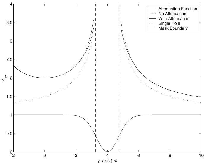
Figure 1: The attenuation function, ${}_{1}B=1-\exp(-\ell_{1}^{4}/2\sigma^{2})$, used to calculate our initial data solutions. To indicate the effect of the attenuation function in a binary black hole system, we also plot the the background metric function $\tilde{g}_{yy}$ in the vicinity of one hole with and without attenuation. The Schwarzschild black holes are placed along the $y$-axis at $\pm 4m$. Here $\ell_{1}$ is the coordinate distance from the center of the second black hole, and the attenuation function width is $\sigma=m^{2}$.

A small volume containing the singularity is masked from the computational domain. This volume is specified by choosing a threshold value for the Ricci scalar, typically for $|R|\geq 2/m^{2}$. For a single Schwarzschild black hole, this gives a spherical mask with a radius $r\simeq 0.73~{}m$. In all cases the masked region lies well within apparent horizons in the solved data. In practice we find that a small attenuation region (also inside the apparent horizon) is necessary to achieve a smooth solution of the elliptic initial data equations near the mask; see Section II.D below. Figures 2 and 3 show the Hamiltonian and momentum constraints for the background space with and without attenuation. We have not varied the masking condition to determine what effect the size of the mask has on the global solution. As mentioned below, Pfeiffer et al. have investigated this point Pfeiffer2 .

Figure 2: The Hamiltonian constraint (units $m^{-2}$) calculated for the background space for two identical Schwarzschild black holes. The black holes are located on the $y$-axis at $y=\pm 4$ m, and have zero initial velocity. The solid curve is the background behavior of the constraint without using attenuation functions, and the dashed curve is the constraint with attenuation and $\sigma=m^{2}$. The masked region is within the radius $r~{}~{}\widetilde{<}~{}~{}0.73m$. It can be seen that attenuation does not necessarily reduce the constraint, but does smooth it.

Figure 3: The $y$-component of the momentum constraint (units $m^{-2}$) calculated for the background space of two identical Schwarzschild black holes. The black holes are located on the $y$-axis at $y=\pm 4~{}m$, and have zero initial velocity. The solid curve is the background behavior of the constraint without using attenuation functions, and the dashed curve is the constraint with attenuation and $\sigma=m^{2}$.

III.4 Generating the physical spacetime

The superposition of Kerr-Schild data described in the previous section does not satisfy the constraints, Eqs. (2)–(3), and hence are not physical. A physical spacetime can be constructed by modifying the background fields with new functions such that the constraints are satisfied. We adopt the conformal transverse-traceless method of York and collaborators YP which consists of a conformal decomposition and a vector potential that adjusts the longitudinal components of the extrinsic curvature. The constraint equations are then solved for these new quantities such that the complete solution fully satisfies the constraints.

The physical metric, $g_{ij}$, and the trace-free part of the extrinsic curvature, $A_{ij}$, are related to the background fields through a conformal factor

$$g_{ij} = \phi^{4}\tilde{g}_{ij},$$ (27)

$$A^{ij} = \phi^{-10}(\tilde{A}^{ij}+\tilde{(lw)}^{ij}),$$ (28)

where $\phi$ is the conformal factor, and $\tilde{(lw)}^{ij}$ will be used to cancel any possible longitudinal contribution to the superposed background extrinsic curvature. $w^{i}$ is a vector potential, and

$$\tilde{(lw)}^{ij}\equiv\tilde{\nabla}^{i}w^{j}+\tilde{\nabla}^{j}w^{i}-\frac{2}{3}\tilde{g}^{ij}\tilde{\nabla_{k}}w^{k}.$$ (29)

The trace $K$ is taken to be a given function

$$K=\tilde{K}.$$ (30)

Writing the Hamiltonian and momentum constraint equations in terms of the quantities in Eqs. (27)–(30), we obtain four coupled elliptic equations for the fields $\phi$ and $w^{i}$ YP :

$$\tilde{\nabla}^{2}\phi = (1/8)\big{(}\tilde{R}\phi+\frac{2}{3}\tilde{K}^{2}\phi^{5}-$$ (31)

$$\phi^{-7}(\tilde{A}{{}^{ij}}+(\tilde{lw})^{ij})(\tilde{A}_{ij}+(\tilde{lw})_{ij})\big{)},$$

$$\tilde{\nabla}_{j}(\tilde{lw})^{ij} = \frac{2}{3}\tilde{g}^{ij}\phi^{6}\tilde{\nabla}_{j}K-\tilde{\nabla}_{j}\tilde{A}{{}^{ij}}.$$ (32)

III.5 Boundary Conditions

A solution of the elliptic constraint equations requires that boundary data be specified on both the outer boundary and the surfaces of the masked regions. This contrasts with the hyperbolic evolution equations for which excision can in principle be carried out without setting inner boundary data since no information can propagate out of the holes. Boundaries in an elliptic system, on the other hand, have an immediate influence on the entire solution domain. Using the attenuation functions, we can choose simple conditions, $\phi=1$ and $w^{i}=0$, on the masked regions surrounding the singularities. In practice this inner boundary condition is not completely satisfactory because it generates small discontinuities in the solution at this boundary. These discontinuities are small relative to the scales in the problem, and are contained within the horizon. We have made no attempt to determine their global effect on the solution. Pfeiffer et al. Pfeiffer2 report a similar observation, and note that the location of the boundary does affect some aspects of the solution, though it has little effect on the fractional binding energy or the location of the ISCO.

The outer boundary conditions are more interesting. Several physical quantities of interest, e.g., the ADM mass and momenta, are global properties of the spacetime, and are calculated on surfaces near the outer boundary of the computational grid. Hence the outer boundary conditions must be chosen carefully to obtain the proper physics. We base our outer boundary conditions on an asymptotic expansion of the Kerr-Schild metric, which relies on the ADM mass and momentum formulæ to identify the physically relevant terms at the boundaries. We first review these expansions and formulæ.

An asymptotic expansion of the Kerr-Schild metric ($\rho\gg m$) gives

$$r = \rho\left(1+{\rm O}(\rho^{-2})\right),$$ (33)

$$H = m/\rho\left(1+{\rm O}(\rho^{-2})\right),$$ (34)

$$l_{i} = n_{i}+\frac{a^{c}\epsilon_{ijc}n^{j}}{\rho}+{\rm O}(\rho^{-2}),$$ (35)

where $n_{i}=n^{i}=x^{i}/\rho$. (This is the only place where we do not use the 3-metric to raise and lower indices, and $n_{i}n^{i}=1$). $a^{c}$ is the Kerr spin parameter with a general direction: $a^{c}=a\hat{a}^{c}$. The shift (Eq. 12) is asymptotically

$$\beta_{i}=\frac{2m}{\rho}\left(n_{i}+a^{c}\frac{\epsilon_{ijc}n^{j}}{\rho}\right)+{\rm O}(\rho^{-3}).$$ (36)

The asymptotic expansion of the extrinsic curvature in the stationary Kerr-Schild form (cf. Eq. (14)) is

$$\alpha K_{ab} = \frac{2m}{\rho^{2}}\left(-2n_{a}n_{b}+\delta_{ab}\right)$$ (37)

$$\hskip 2.84544pt-\frac{3m}{\rho^{3}}a^{c}\left(\epsilon_{ajc}n_{b}+\epsilon_{bjc}n_{a}\right)n_{j}$$

$$\hskip 2.84544pt+\frac{6m^{2}}{\rho^{3}}\left(n_{a}n_{b}-\frac{2}{3}\delta_{ab}\right)+{\rm O}(\rho^{-4}).$$

The terms proportional to $a^{c}/\rho^{3}$ in this expression arise from the transverse components of $\beta^{a}$ ($\beta_{a}n^{a}=0$); the terms of ${\rm O}(\rho^{-3})$ independent of $a^{c}$ arise from the affine connection. Note that $\alpha=1+{\rm O}(\rho^{-1})$, and will not affect the ADM estimates below.

The ADM formulæ are evaluated in an asymptotically flat region surrounding the system of interest, and in Cartesian coordinates they are

$$M_{{\rm ADM}} = \frac{1}{16\pi}\oint\left(\frac{\partial g_{ji}}{\partial x^{j}}-\frac{\partial g_{jj}}{\partial x^{i}}\right){\rm d}S^{i},$$ (38)

$$P^{{\rm ADM}}_{k} = \frac{1}{8\pi}\oint\left(K_{ki}-K^{b}{}_{b}\delta_{ki}\right){\rm d}S^{i},$$ (39)

$$J^{{\rm ADM}}_{ab} = \frac{1}{8\pi}\oint\left(x_{a}K_{bi}-x_{b}K_{ai}\right){\rm d}S^{i},$$ (40)

for the mass, linear momentum, and angular momentum of the system respectively Wald ; note4 . (All repeated indices are summed.) The mass and linear momentum together constitute a 4-vector under Lorentz transformations in the asymptotic Minkowski space, and the angular momentum depends only on the trace-free components of the extrinsic curvature.

To compute the ADM mass and momentæfor a single, stationary Kerr-Schild black hole, we evaluate the integrals on the surface of a distant sphere. The surface element then becomes $dS^{i}=n^{i}\rho^{2}{\rm d}\Omega$, where $n^{i}$ is the outward normal and ${\rm d}\Omega$ is the differential solid angle. we need to evaluate the metric only to order ${\rm O}(\rho^{-1})$; the differentiation in Eq. (38) guarantees that terms falling off faster than $\rho^{-1}$ do not contribute to the integration. The integrand is then $\frac{4m}{\rho^{2}}n_{i}\rho^{2}n^{i}\,{\rm d}\Omega$ and the integration yields the expected ADM mass $M_{ADM}=m$. The ADM linear momentum requires only the leading order of of $K_{ab}$, ${\rm O}(\rho^{-2})$; terms falling off faster than this do not contribute. The integrand of Eq. (39) then becomes $-\frac{4m}{\rho^{2}}n_{a}n_{b}n^{b}\rho^{2}\,{\rm d}\Omega,$ yielding zero for the 3-momentum, as expected for a non-moving black hole.

At first blush, the integral for the ADM angular momentum Eq. (40) appears warrant some concern: To leading order $K_{ab}$ is ${\rm O}({\rho^{-2}})$, and the explicit appearance of $x_{a}$ in the integrand suggests that it grows at infinity as ${\rm O}(\rho)$, leading to a divergent result. However, inserting the leading order term of $K_{ab}$ for a single, stationary Kerr-Schild black hole into the integrand of Eq. (40), we find that the integrand is identically zero. The ${\rm O}({\rho^{-2}})$ terms of $K_{ab}$ contain the quantities $n_{a}n_{b}$ and $\delta_{ab}$, which separately cancel because of the antisymmetric form of Eq. (40), and a divergent angular momentum is avoided. Including the ${\rm O}(\rho^{-3})$ terms of $K_{ab}$, we find $J^{\rm ADM}_{ab}=\epsilon_{abc}a^{c}m$; the symmetry of the other ${\rm O}(m^{2}\rho^{-3})$ terms again means they do not contribute. This result for $J^{\rm ADM}_{ab}$ thus depends on terms in the integrand proportional to $a$ that arise from corresponding terms in $\beta^{i}$ proportional to $q^{i}$ where $q^{a}$ is a unit vector transverse to the radial direction, $q^{a}n_{a}=0$. Only these terms contribute to the angular momentum integral; in particular those terms in $\beta^{i}$ proportional to $n^{i}/\rho$ do not contribute.

The ADM mass and momenta are Lorentz invariant. For a single, boosted black hole, we naturally obtain $M_{\rm ADM}=\gamma m$ and $P_{\rm ADM}=\gamma mv$. The background spacetime for multiple black holes is constructed with a superposition principle, and the ADM quantities are linear in deviations about flat space at infinity. Thus the ADM formulæ, evaluated at infinity in the superposition, do yield the expected superposition. For example, given two widely separated black holes boosted in the $x$-$y$ plane with spins aligned along the $z$-axis, we have

$$\tilde{M}_{\rm ADM} = {}_{1}\gamma{}_{1}m+{}_{2}\gamma{}_{2}m,$$ (41)

$$\tilde{P}^{\rm ADM}_{i} = 0,$$ (42)

$$\tilde{J}^{\rm ADM}_{12} = {}_{1}\gamma\left({}_{1}m{}_{1}v{}_{1}b+{}_{1}m{}_{1}a\right)+{}_{2}\gamma\left({}_{2}m{}_{2}v{}_{2}b+{}_{2}m{}_{2}a\right),$$ (43)

where ${}_{1}b$ and ${}_{2}b$ are impact parameters note1 , and the tilde ( $\tilde{}$ ) superscript indicates that these quantities are calculated with the background tensors $\tilde{g}_{ab}$ and $\tilde{K}_{ab}$. This superposition principle for the ADM quantities in the background data is one advantage of conformal Kerr-Schild initial data. (Note, in choosing the center of momentum frame for the computation, $P^{{\rm ADM}}_{i}=0$ is a condition for setting the background data.)

Consider now the ADM integrals for the solved data. The Hamiltonian constraint becomes an equation for the conformal factor, $\phi$. As this equation is a nonlinear generalization of Poisson’s equation, asymptotic flatness in the full, solved metric requires that

$$\phi\longrightarrow 1+\frac{C}{2\rho}+{\rm O}(\rho^{-2}),$$ (44)

where $C$ is a (finite) constant. This leads to our outer boundary condition for $\phi$, namely

$$\partial_{\rho}\left(\rho(\phi-1)\right)|_{\rho\rightarrow\infty}=0.$$ (45)

Furthermore, the linearity of the ADM mass integral gives

$$M_{\rm ADM}\mbox{(solved)}={}_{1}\gamma{}_{1}m+{}_{2}\gamma{}_{2}m+C.$$ (46)

(Here the absence of a tilde ( $\tilde{}$ ) indicates that this mass is calculated using the solved $g_{ab}$.) At this point we cannot predict even the sign of $C$, though $|C|$ is expected to be small for widely separated holes. If $|C|\to\infty$, then the boundary condition Eq. (45) would fail. The existence of solutions using this condition, however, provides evidence that this possibility does not occur.

The boundary condition for $w^{i}$ is more subtle. A priori, we expect $w^{i}\rightarrow 0$ at infinity, but a physically correct solution on a finite domain requires that we understand how $w^{i}$ approaches this limit at infinity. We construct our boundary conditions on $w^{k}$ by demanding that the ADM angular momentum of the full (solved) system be only finitely different from that of the background (superposed) data. That is, given that $\{\tilde{g}_{ab},\tilde{K}_{ab}\}$ and $\{g_{ab},K_{ab}\}$ have finite differences at infinity, we demand that $J_{ab}-\tilde{J}_{ab}$ also be finite. Using (Eq. (28)) and (Eq. (40)), we find for the difference in angular momentum

$$J_{ab}-\tilde{J}_{ab}=\frac{1}{8\pi}\oint\left(x_{a}\nabla_{(b}w_{i)}-x_{b}\nabla_{(a}w_{i)}\right){\rm d}S^{i}\,.$$ (47)

($\phi\to 1$ at infinity, and there is no difference at this order between conformal and physical versions of $w^{i}$ and $g_{ab}$ at infinity.)

We have already evaluated an integral of this form, in the discussion of the Kerr angular momentum (see Eq. (40) and Eq. (37)), where we expressed $K_{ab}$ in terms of the Kerr-Schild shift vector. In that analysis, we noted that falloff of the form

$$w_{i}\longrightarrow\frac{C_{1}}{\rho}n_{i}+\frac{C_{2}}{\rho^{2}}q_{i}+{\rm O}(\rho^{-3}),$$ (48)

with $C_{1}$ and $C_{2}$ constant, and $q_{i}n^{i}=0$, will give a finite contribution to the angular momentum. We therefore take as boundary conditions:

$$\partial_{\rho}(\rho w^{i}n_{i})=0$$ (49)

$$\partial_{\rho}\left(\rho^{2}w^{i}(\delta_{ij}-n_{i}n_{j})\right)=0\,.$$ (50)

Figures (4)–(6) display $\phi$ and $w^{i}$ for a simple configuration. In this case the elliptic equations were solved on a domain of $\pm 10~{}m$ along each axis with resolution $\Delta x=m/8$. As can be seen in these figures, the functions $\phi$ and $w^{i}$ actually result in little adjustment to the background configurations. Also note that the radial component of $w^{i}$, $w^{i}n_{i}$, is the dominant function. In the graphs plotted here, which give the functions along the $y$-axis, we find of $||w^{y}||_{\infty}\approx 0.03$, while $||w^{x}||_{\infty}\approx 3\times 10^{-3}$, and $||\phi-1||_{\infty}\approx 0.013$. Because of the symmetry of the configuration, $||w^{z}||_{\infty}$ is much smaller. Analytically, $w^{z}=0$ on the $y$-axis; computationally we find $||w^{z}||_{\infty}\approx 5\times 10^{-7}$. In fact we find in general that the radial component of $w^{i}$ is the dominant function in all directions, consistent with our boundary conditions, and consistent with the finding that solution of the constraints has small effect on the computed angular momentum. Of course the corrections $\phi$ and $w^{i}$ would be expected to be larger, for data describing holes closer together. We show below that this data setting method leads to generically smaller corrections than found in other methods, thus allowing closer control of the physical content of the data.

Figure 4: $\phi$ along the y-axis connecting two nonspinning holes with orbital angular momentum. The holes are boosted in the $\pm$ x direction with $v=0.196$ and are separated by $10$ M. Note that $\phi$ is very close to unity everywhere.

Figure 5: $w^{x}$ for the same configuration as in Figure 4.

Figure 6: $w^{y}$ for the same configuration as in Figure 4. $w^{z}$ is numerically zero as expected by symmetry.

IV Binding Energy in Initial Data

As a first step towards understanding the physical content of initial data sets, we examine in this section the effect of the presence of a second hole on the horizon areas of a first hole and on global features such as the ADM integrals and the binding energy of the pair. This analysis is carried out for non-spinning holes to first order in the binding energy. A comparison to the Newtonian result indicates that the Kerr-Schild background superposition data contain the appropriate physical information at this level. We then consider possible spin-related phenomena, estimate their magnitude, and discuss their possible effect near the ISCO.

IV.1 Binding energy in Brill-Lindquist data

Before discussing the conformal Kerr-Schild data, we first consider Brill-Lindquist data for two non-moving Schwarzschild black holes Brill . These data are conformally flat, and $K_{ab}=0$. The momentum constraints are trivially satisfied, and the Hamiltonian constraint is solved for a conformal factor: $\phi=1+m/(2r)+m^{\prime}/(2r^{\prime})$. Here the two mass parameters are $m$, and $m^{\prime}$, and $r$ and $r^{\prime}$ are the distances in the flat background from the holes $m$ and $m^{\prime}$.

We find that the apparent horizon areas in the solved data correspond to

$$M_{\rm AH}+M_{\rm AH}^{\prime}=m+m^{\prime}+\frac{mm^{\prime}}{\ell}+{\rm O}(\ell^{-2}).$$ (51)

The subscript “$\rm AH$” indicates masses computed from apparent horizon areas, and the separation in the flat background space is $\ell$ cadez . We assume that this mass (computed from apparent horizons) is close to the total intrinsic mass of the black holes (which is given by a knowledge of the spin—here zero—and the area of the event horizon). The binding energy, ${E_{b}}$, can be computed as the difference of the ADM mass observed at infinity and the sum of the horizon masses:

$${E_{b}}=M_{{\rm ADM}}-M_{\rm AH}-M^{\prime}_{\rm AH}.$$ (52)

For Brill-Lindquist data $M_{{\rm ADM}}=m+m^{\prime}$, so that

$${E_{b}}=-\frac{Gmm^{\prime}}{\ell}+{\rm O}(\ell^{-2})\,,$$ (53)

which is the Newtonian result.

IV.2 Binding Energy in Superposed Kerr-Schild Data

We now calculate the binding energy in superposed Kerr-Schild data (set according to our conformal transverse-traceless approach) for a non-moving Schwarzschild black hole at the origin, and a second such hole at coordinate distance $\ell$ away. ($\ell$ is measured in the flat space associated with the data construction.) We compute the area of the hole at the origin to first order and find that the Newtonian binding energy already appears in the the background data prior to solving the constraints. Thus, we have an argument justifying the result noted at the end of Section III.5: solving the elliptic constraint equations leads to small corrections to the Kerr-Schild background data.

Let both holes be placed on the $z$-axis; the first hole with mass parameter $m$ at the origin, and a second hole with mass parameter $m^{\prime}$ at $z=\ell$. The holes are well separated, and we expand all quantities about the origin in powers of $\epsilon\equiv m^{\prime}/\ell$ with $\epsilon\ll 1$. Using Schwarzschild coordinates labeled $(r,\theta,\phi)$ (cf. Eq. (4)–Eq. (9) for $a=0$), the background metric tensor is

$$\tilde{g}_{rr} = 1+\frac{2m}{r}+2\epsilon\cos^{2}\theta,$$ (54)

$$\tilde{g}_{r\theta} = -2\epsilon r\sin\theta\cos\theta,$$ (55)

$$\tilde{g}_{\theta\theta} = r^{2}+2\epsilon r^{2}\sin^{2}\theta,$$ (56)

$$\tilde{g}_{\phi\phi} = r^{2}\sin^{2}\theta,$$ (57)

with all other components zero. The extrinsic curvature of the second hole, ${}_{2}K_{ab}$, is of ${\rm O}(\epsilon^{2})$ at the origin, and we have simply $\tilde{K}_{ab}={}_{1}K_{ab}$. Similarly, the trace of the extrinsic curvature is $\tilde{K}={}_{1}K$. Finally, the non-zero components of $\tilde{A}_{ab}$ are

$$\tilde{A}_{rr} = -\frac{2c_{2}}{r^{2}}\left(1+2\frac{m}{r}+2\epsilon\cos^{2}\theta\right),$$ (58)

$$\tilde{A}_{r\theta} = \epsilon\frac{c_{2}}{r}\sin\theta\cos\theta,$$ (59)

$$\tilde{A}_{\theta\theta} = c_{2}\left(1+2\epsilon\sin^{2}\theta\right),$$ (60)

$$\tilde{A}_{\phi\phi} = c_{2}\sin^{2}\theta.$$ (61)

where

$$c_{2}\equiv\frac{2M}{3}\sqrt{\frac{\rho}{\rho+2M}}\frac{(2r+3m)}{(r+2m)}.$$ (62)

While $\tilde{K}_{ab}$ is not a function of $\epsilon$, and hence contains no information about the second hole, perturbative quantities do appear in $\tilde{A}_{ab}$. This perturbation in $\tilde{A}_{ab}$ arises because we sum the mixed-index components of ${}_{A}A^{c}_{b}$, and because the full background metric, involving terms from each hole, is involved in the symmetrization in Eq. (23).

To calculate the binding energy we first find the apparent horizon area of the local hole. For a single Schwarzschild hole, the horizon is spherical and located at $\rho_{{\rm H}}=2m$; the area of the horizon is $16\pi m^{2}$. The effect of the second hole is to distort the horizon along the $z$-axis connecting them, and we define a trial apparent horizon surface as $f=0$, where

$$f=\rho-2m-\sum_{l}a_{l}P_{l}(\cos\theta)\,.$$ (63)

The expansion of $f$ in Legendre polynomials, $P_{l}$, expresses the distortion of the local horizon away from the zero-order spherical result. This expansion includes a term describing a constant “radial” offset in the position of the apparent horizon, $a_{0}P_{0}$. This and the other terms defining the surface have the expected magnitude, $a_{l}={\rm O}(m\epsilon)$. We solve for the horizon by placing this expression for the surface into the apparent horizon equation

$$\nabla_{i}s^{i}+A_{ab}s^{a}s^{b}-\frac{2}{3}K=0,$$ (64)

where $s^{i}$ is the unit normal to the trial surface

$$s_{i}=\frac{f_{,i}}{\sqrt{g^{ab}f_{,a}f_{,b}}}.$$ (65)

The apparent horizon equation is solved to first order, ${\rm O}(\epsilon)$. One must evaluate the equation at the new (perturbed) horizon location. Let $F$ represent the left-hand side of the apparent horizon equation (Eq. (64)), $\rho_{0}=2m$ is the horizon surface of the single, unperturbed hole, and $\rho_{\rm H}(\theta)$ is the new perturbed horizon. We expand $F$ to first order as

$$F(\rho_{\rm H}(\theta))=F_{0}(\rho_{0})+\frac{\partial F}{\partial\rho}\biggr{|}_{\rho_{0}}\sum a_{l}P_{l}\,=0.$$ (66)

Solving (Eq. (64)), the only nonzero coefficients in Eq.(63) are $a_{0}=mm^{\prime}/(3\ell),$ $a_{2}=-mm^{\prime}/(2\ell)$. Integrating the determinant of the perturbed metric over the horizon surface, $\rho=2m+\sum_{l}a_{l}P_{l}(\cos\theta)$, we find the area of the apparent horizon to be

$$A_{\rm H}=16\pi\left(m+\frac{mm^{\prime}}{2\ell}\right)^{2}+{\rm O}\left(m^{2}(m^{\prime}/\ell)^{2}\right),$$ (67)

corresponding to a horizon mass of $M_{\rm H}=m+mm^{\prime}/(2\ell)$ to Newtonian order, ie to order ${\rm O}(\epsilon)={\rm O}(\ell^{-1})$.

In this nonmoving case the total ADM mass is just $M_{\rm ADM}=m+m^{\prime}$. This leads to the Newtonian binding energy at this order

$${E_{b}}=-\frac{mm^{\prime}}{\ell}.$$ (68)

Because we work only to lowest order in $\epsilon$, Eq. (68) had to result in an expression of ${\rm O}(m\epsilon)$, but it did not have to have a coefficient of unity. Both the conformally flat and conformally Kerr-Schild data contain the Newtonian binding energy. However, this result is obtained in the superposed background Kerr-Schild metric, while the Brill-Lindquist and Čadež data give the correct binding energy only after solving the elliptic constraints. This is consistent with the small corrections introduced by $\phi$ and $w^{i}$ ($\phi\sim 1$, $|w^{i}|\ll 1$) in the solved Kerr-Schild data (see Section III.5). This fact—that for a superposed Kerr-Schild background the solution of the full elliptic problem modifies the data (and the mass/angular momentum computations) only slightly—demonstrates how powerful this choice of data can be.

Furthermore, the Newtonian form of the binding energy ($\epsilon\ll 1$) means the correct classical total energy is found for orbiting situations. If the holes have nonrelativistic motion, their individual masses are changed by order $\gamma\approx 1+{\rm O}(v^{2})=1+{\rm O}(\epsilon)$. The binding energy, which is already ${\rm O}(\epsilon)$ and is proportional to the product of the masses, is changed only at order ${\rm O}(\epsilon^{2})$. The ADM mass, on the other hand, measures $\gamma m$, and $M_{\rm ADM}$ will be increased by $mv^{2}/2$ (an ${\rm O}(\epsilon)$ increase) for each hole, leading to the correct Newtonian energetics for the orbit.

The apparent horizon is the only structure available to measure the intrinsic mass of a black hole. Complicating this issue is the intrinsic spin of the black hole; the relation is between horizon area and irreducible mass:

$$A_{\rm H}=16\pi m_{irr}^{2}=8\pi m\left(m+\sqrt{(m^{2}-a^{2})}\right)$$ (69)

As Eq. (69) shows, the irreducible mass is a function of both the mass and the spin, and in general we cannot specify the spin of the black holes. For axisymmetric cases Ashtekar’s isolated horizon paradigm Dreyer gives a way to measure the spin locally. We do not pursue the point here since we investigate generic and typically non-axisymmetric situations.

IV.3 Spin effects in Approximating Inspiral With Initial Data Sequences

We have seen that the initial data contain the binding energy in a multiple black hole spacetime. This information can be used to deduce some characteristics of the orbital dynamics, particularly the radius of the circular orbit, $\ell$, and the orbital frequency, $\omega$. Given a sequence of initial data slices with decreasing separations, we determine ${E_{b}}$ for each slice. The circular orbit is found where

$$\frac{\partial{E_{b}}}{\partial\ell}\biggr{|}_{J}=0.$$ (70)

The separation at the ISCO orbit, $\ell_{\rm ISCO}$, lies at the boundary between binding energy curves which have a minimum, and those that do not. The curve for the ISCO has an inflection point:

$$\frac{\partial^{2}{E_{b}}}{\partial\ell^{2}}\biggr{|}_{J}=0.$$ (71)

The angular frequency is given by

$$\omega_{\rm ISCO}=\frac{\partial{E_{b}}}{\partial J}.$$ (72)

The attempt to model dynamical inspiral seems secure for large separation ($\ell>15m$), though surprises appear even when the holes are very well separated. For instance, Eq. (67) above shows that compared to the bare parameter values, the mass increase is equal for the two holes in a dataset. Thus the smaller hole is proportionately more strongly affected than the larger one is.

The physically measurable quantity in question is the frequency (at infinity) Eq. (72) associated with the last orbit prior to the plunge, the ISCO. This may be impossible to determine by the initial data set method.

To begin with, isolated black holes form a 2-parameter set (depending on the mass parameter $m$, and the angular momentum parameter, $j=ma$). For isolated black holes without charge the parameters $\{m,j\}$ uniquely specify the hole. They are equal, respectively, to the physical mass and angular momentum. Every method of constructing multiple black hole data assigns parameter values ${}_{B}m$ and ${}_{B}j$ to each constituent ${}_{B}(hole)$ in the data set.

There is substantial ambiguity involving spin and mass in setting the black hole data. One must consider the evolutionary development of the black hole area and spin. This is a real physical phenomenon which contradicts at some level the usual assumption of invariant mass and spin. A related concern arises because it is only the total ADM angular momentum that is accessible in the data, whereas one connects to particle motion via the orbital angular momentum.

Consider the behavior of the individual black hole spin and mass in an inspiral. For widely separated holes, because the spin effects fall off faster with distance than the dominant mass effects do, we expect the spin to be approximately conserved in an inspiral. Therefore it should also be constant across the initial data sets representing a given sequence of orbits. But when the holes approach closely, the correct choice of spin parameter becomes problematic also.

Newtonian arguments demonstrate some of the possible spin effects. In every case they are a priori small until the orbits approach very closely. However, at estimates for the ISCO, the effects begin to be large, and result in ambiguities in setting the data (see Price and Whelan P+W ). We will consider these effects in decreasing order of their magnitude.

For two holes, each of mass $m$ in Newtonian orbit with a total separation of $\ell$, the orbital frequency is

$$m\omega=\sqrt{2}(m/\ell)^{(3/2)}.$$ (73)

From recent work by Pfeiffer et al. Pfeiffer , the estimated ISCO frequency is of order $m\Omega=0.085$, corresponding to $\ell\approx 6.5\,m$ in this Newtonian approach.

To compare this frequency, Eq. (73), to an intrinsic frequency in the problem, we take the lowest (quadrupole) quasi-normal mode of the final merged black hole (of mass $2m$) which has frequency $2m\omega_{0}\approx 0.37$; the quadrupole distortion is excited at twice the orbital frequency. (We are using the values for a Schwarzschild black hole in this qualitative analysis.) The driving frequency equals the quasi-normal mode frequency when $\ell\approx 4\,m$, as might be expected.

To consider effects linked to the orbital motion on the initial configurations, we can first treat the effect of imposing corotation. While we show below that corotation is not physically enforced except for very close orbits, it is a fact that certain formulations, for instance versions of the “thin sandwich” with a helical Killing vector, require corotation in their treatment. For any particular initial orbit, corotation is certainly a possible situation.

In corotation, then, with Eq. (73), for each hole:

$$J=ma=I\omega=4m^{2}(m\omega).$$ (74)

The result for the moment of inertia $I=4m^{3}$ is the Schwarzschild value MTW ; membrane . Thus

$$a=4m\sqrt{2}(m/\ell)^{(3/2)}.$$ (75)

Assume $a/m\ll 1$, and compute the area of this black hole MTW :

$$A=8\pi m(m+\sqrt{m^{2}-a^{2}})\\ \approx 16\pi m^{2}(1-(a/m)^{2}/4).$$ (76)

The horizon mass computed from this area is

$$\sqrt{A/(16\pi)}\approx m(1-4(m/\ell)^{3}).$$ (77)

At our estimate of the ISCO orbit, $\ell_{\rm ISCO}\approx 6\,m$, this effect is of order of 10% of the Newtonian binding energy, distinctly enough to affect the location of the ISCO.(At $\ell_{\rm ISCO}\approx 6\,m$, $a/m\approx 0.3$ for corotation).

Two more physical effects are not typically considered in setting data. They are frame dragging, and tidal torquing. Within our Newtonian approximations, we will find that these effects are small, but not zero as the orbits approach the ISCO. In full nonlinear gravity these effects could be substantial precisely at the estimated ISCO.

The frame dragging is the largest dynamical effect. The orbiting binary possesses a net angular momentum. For a rotating mass (here the complete binary system) the frame dragging angular rate is estimated as the rotation rate times the gravitational potential at the measurement point MTW . Hence

$$m\Omega_{\rm{drag}}=m\omega\left(\frac{2m}{\ell}\right)\approx\left(\frac{m}{\ell}\right)^{\frac{5}{2}}\approx\frac{a}{4m}.$$ (78)

This is $a/m$ of order 1% at $\ell=10m$; of order 4% at $\ell=6m$.

The tidal torquing and dissipative heating of the black holes can be similarly estimated. As the two holes spiral together, the tidal distortion from each hole on the other will have a frequency which is below, but approaching the quasi-normal frequency. Just as for tidal effects in the solar system, there will be lag in the phase angle of the distortion, which we can determine because the lowest quasi-normal mode is a dissipative oscillator, driven through the tidal effects at twice the orbital frequency:

$$\ddot{q}+2\gamma\dot{q}+\omega_{0}^{2}q=F(\omega).$$ (79)

Here $m^{2}q$ is the quadrupole moment of the distorted black hole. The parameter $\gamma$ is (for a Schwarzschild hole of mass $2m$)) about $2m\gamma=0.089$. In Eq. (79) the driving acceleration $F(\omega)$ is identified with the tidal distortion acceleration. We evaluate it at zero frequency:

$$q = F(\omega=0)/\omega_{0}^{2}$$ (80)

$$\approx \frac{m}{\ell^{3}}.$$ (81)

The lagging phase, for driving frequency $2\omega\ll\omega_{0}$, is easily computed to be

$$\phi \approx 4\gamma\frac{\omega}{\omega_{0}^{2}}$$ (82)

$$= 4\left(\frac{\gamma}{\omega_{0}}\right)\left(\frac{\omega}{\omega_{0}}\right)$$ (83)

This lagging tidal distortion will produce a tidal torque on the black hole, which we can approximate using a combination of Newtonian and black hole ideas. The most substantial approximation is that the torque arises from a redistribution of the mass in the “target” black hole, of amount $\Delta m=mm^{2}q=m(m/\ell)^{3}$. This mass has separation $\approx 4m$. Thus the torque on the hole is

$$\tau = \sin\phi\times(\mbox{lever arm})\times\Delta F$$

$$= \sin\phi\times(4m)\times(\Delta m2m^{2}/\ell^{3})$$

$$= 8\sin\phi m(m/\ell)^{6}$$

$$\approx 32(\gamma/\omega_{0})(\omega/\omega_{0})m(m/\ell)^{6}$$

$$\approx 60m(m/\ell)^{15/2}.$$

What is most important is the effect of this torque on the angular momentum of the hole over the period of time it takes the orbit to shrink from a very large radius. To accomplish this, we use the inspiral rate (calculated under the assumption of weak gravitational radiation from the orbit; see MTW ):

$$\frac{d\ell}{dt}=-\frac{128}{5}\left(\frac{m}{\ell}\right)^{3}$$ (85)

Thus

$$\frac{dJ}{d\ell} = \tau\frac{dt}{d\ell}$$ (86)

$$= -\frac{5\tau}{128}\left(\frac{m}{\ell}\right)^{-3}$$ (87)

$$\approx -2m\left(\frac{m}{\ell}\right)^{9/2},$$ (88)

and

$$J(\ell)\approx m^{2}\left(\frac{m}{\ell}\right)^{7/2};$$ (89)

assuming that there is minimal mass increase from the associated heating (which we discuss just below), this identifies the induced spin parameter $a=m(m/\ell)^{7/2}$ for an inspiral from infinity.

The estimate $a=m(m/\ell)^{7/2}$ for an inspiral from infinity assumes the mass of the hole has not changed significantly in the inspiral. By considering the detailed behavior of the shear induced in the horizon by the tidal perturbation, the growth in the black hole mass can be estimated membrane as

$$\frac{dm}{dt} = \omega\frac{dJ}{dt},$$ (90)

leading to a behavior

$$\Delta m(\ell)\approx 5m\left(\frac{m}{\ell}\right)^{5};$$ (91)

Consequently, the change in mass can be ignored until the holes are quite close. However, the point is that these Newtonian estimates lead to possible strong effects just where they become unreliable, and just where they would affect the ISCO.

These results are consistent with similar ones of Price and Whelan P+W , who estimated tidal torquing using a derivation due to Teukolsky TeukThesis . That derivation assumes the quadrupole moment in the holes arises from their Kerr character, which predicts specific values for the quadrupole moment, as a function of angular momentum parameter $a$.

Finally we consider an effect on binding energy shown by Wald and also by Dain. Wald directly computes the force for stationary sources with arbitrarily oriented spins. He considered a small black hole as a perturbation in the field of a large hole. The result found WaldPRD was

$${E_{b}}=-\frac{mm^{\prime}}{\ell}-\left(\frac{\vec{S}\cdot\vec{S^{\prime}}-3(\vec{S}\cdot\hat{n})(\vec{S^{\prime}}\cdot\hat{n})}{\ell^{3}}\right).$$ (92)

Here, $\vec{S}$, $\vec{S}^{\prime}$ are the spin vectors of the sources and $\hat{n}$ is the unit vector connecting the two sources. Dain Dain , using a definition of intrinsic mass that differs from ours, finds binding energy which agrees with Wald’s Eq. (92) at ${\rm O}(\ell^{-3})$. This is discussed further in Section V.2.

V Numerical Results

We now turn to computational solutions of the constraint equations to generate physical data using the superposed Kerr-Schild data. We first discuss the computational code and tests, as well as some of the limitations of the code. Finally, we consider physical conclusions that can be drawn from the results.

V.1 Code Performance

The constraint equations are solved (Eq. (32)) with an accelerated SOR solver NumRecepies . The solution is iterated until the $L_{2}$ norms of the residuals of the fields are less than $10^{-10}$, far below truncation error. Discrete derivatives are approximated with second order, centered derivatives. We are limited to fairly small domains, e.g., $x^{i}\in[-12m,12m]$ for a typical $m/8$ resolution using $193^{3}$ points.

To verify the solution of the discrete equations, we have examined the code’s convergence in some detail. The constraints have known analytical solutions—they should be zero—which allows us to determine the code’s convergence using a solution calculated at two different resolutions. Let $S_{1}$ be a solution calculated with resolution $h_{1}$, and $S_{2}$ be a solution calculated with $h_{2}$, then the convergence factor $c_{12}$ is

$$c_{12}=\frac{\log\left(\frac{||S_{1}||}{||S_{2}||}\right)}{\log\left(\frac{h_{1}}{h_{2}}\right)}$$ (93)

We constructed a conformal background spacetime with two $m=1$ non-spinning black holes separated by $6m$ on the $y$-axis. The elliptic equations were then solved on grids with resolutions of $m/6$, $m/8$, $m/10$ and $m/12$. Tables 1–2 show the convergence factors as a function of resolution for the Hamiltonian constraint and the $x$-component of the momentum constraint, ${\cal C}^{x}$. The convergence for ${\cal C}^{y}$ is nearly identical to ${\cal C}^{x}$, and as the $y$-axis is an axis of symmetry, ${\cal C}^{z}$ is identical to ${\cal C}^{x}$. Figures 7–9 show the convergence behavior of the constraints along coordinate lines. The constraints calculated at lower resolutions are rescaled to the highest resolution by the ratio of resolutions squared. We see second order for all components with the exception of the points nearest to the inner boundary.

Convergence $(c_{ab})$
	$a=m/6$	$a=m/8$	$a=m/10$
$b=m/8$	1.70
$b=m/10$	1.77	1.86
$b=m/12$	1.79	1.86	1.85

Table 1: Convergence data for the Hamiltonian constraint, ${\cal C}^{0}$, for a solution with two $m=1$, non-spinning holes at $x^{i}=(0,\pm 3m,0)$ in the conformal background, and outer boundaries at $x^{i}=\pm 6m$. The solution was calculated at resolutions $m/6$, $m/8$, $m/10$, and $m/12$. The $L_{2}$ norms of ${\cal C}^{0}$ were calculated over the entire volume of the domain using a mask of radius $1m$ around each hole, while the computational mask has a radius of approximately $0.75~{}m$. This larger mask was used to compensate for the slight difference of physical location of the mask at different resolutions. The norms are as follows: $||{\cal C}^{0}(m/6)||_{2}=0.00389054$, $||{\cal C}^{0}(m/8)||_{2}=0.00238321$, $||{\cal C}^{0}(m/10)||_{2}=0.00157387$ and $||{\cal C}^{0}(m/12)||_{2}=0.00112328$.

Convergence $(c_{ab})$
	$a=m/6$	$a=m/8$	$a=m/10$
$b=m/8$	1.93
$b=m/10$	1.99	2.06
$b=m/12$	1.99	2.03	1.99

Table 2: Convergence data for the $x$-component of the momentum constraint, for the same configuration as Table 1. The norms of ${\cal C}^{x}$ are as follows: $||{\cal C}^{x}(m/6)||_{2}=0.00541231$, $||{\cal C}^{x}(m/8)||_{2}=0.00310937$, $||{\cal C}^{x}(m/10)||_{2}=0.00196156$ and $||{\cal C}^{x}(m/12)||_{2}=0.00136514$. Convergence factors were also calculated for ${\cal C}^{y}$ and ${\cal C}^{z}$, and found to be essentially identical to the data shown here, and thus are not given separately.

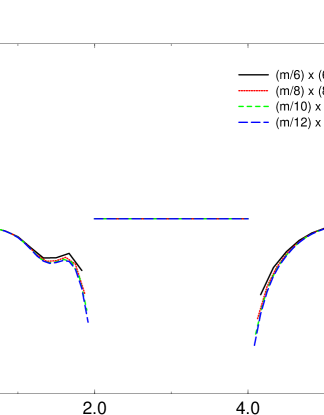
Figure 7: The Hamiltonian constraint (units $m^{-2}$) along $y$-axis after solving the elliptic equations for 4 different levels of resolution. The constraints are rescaled by the ratio of the resolutions squared, showing second order convergence. The two non-spinning, instantaneously stationary holes of $m=1$ are positioned at $\pm 3$ on the $y$-axis.

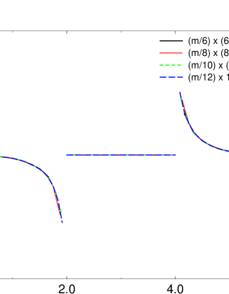
Figure 8: $y$-component of momentum constraint (units $m^{-2}$) along the $y$-axis after solving the elliptic equations for 4 different levels of resolution, showing second order convergence. The background physical situation is the same as in Figure (7). The other momentum constraint components evaluated on this axis are zero by symmetry, both analytically, and computationally (${\rm O}(10^{-12})$).

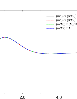
Figure 9: $z$-component of momentum constraint (units $m^{-2}$) along the $z$-axis after solving the elliptic equations for 4 different levels of resolution, showing second order convergence. Other components of the momentum constraint evaluated along this line are zero by symmetry, both analytically and computationally (${\rm O}(10^{-12})$). The background physical situation is the same as in Figure (7). The behavior of the $x$-momentum constraint along the $x$-axis is identical to this Figure, as required by the symmetry of the problem.

Domain	$M_{ADM}$
$\pm$ 8 m	1.942 m
$\pm$ 10 m	1.964 m
$\pm$ 11 m	1.974 m
$\pm$ 12 m	1.980 m

Table 3: Total ADM Mass for two instantaneously stationary, non-spinning holes separated by $6m$ on a grid of discretization $\Delta x=m/8$ for four different domain sizes.

Solutions of elliptic equations are well-known to be dependent on all boundary data. The outer boundary is an artificial boundary, as the the physical spacetime is unbounded. Boundary data for this outer boundary are derived from the asymptotic behavior of a single Kerr black hole. On very large domains these conditions should closely approximate the expected field behavior, but on small domains these boundary data may only crudely approximate the real solution. This error in the boundary data then contaminates the entire solution, as expected for elliptic solutions. Additional error arises in the calculation of the ADM quantities, as spacetime near the outer boundary does not approach asymptotic flatness. As an indication of the error associated with the artificial outer boundaries, we calculated solutions with the same physical parameters on grids of differing sizes. The boundary effects in the $M_{\rm ADM}$ are given in Table 3, and Fig. 10 shows a contour plot of $\phi$ for equal mass, nonspinning, instantaneously stationary black holes with the outer boundaries at $x^{i}=\pm 12m$. As a further demonstration of boundary effects in our solutions, Fig. 11 shows $\phi$ for a configuration examined by Pfeiffer et al. Pfeiffer2 . Their solution, shown in Fig. 8 of Pfeiffer2 , was computed on a much larger domain via a spectral method Kidder . Thus, while we achieve reasonable results, it is important to remember that the boundary effects may be significant. Moreover, we have only considered the effect of outer boundaries, while errors arising from the approximate inner boundary condition have not been examined.

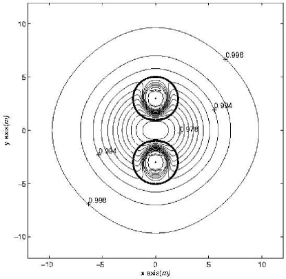
Figure 10: Contour plot of $\phi$ for two instantaneously stationary, non-spinning holes of mass parameter $m=1$. The holes are separated by $6~{}m$ along the y-axis. The bold circles indicate the apparent horizons.

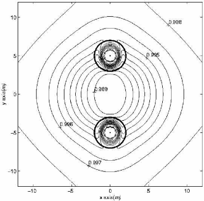
Figure 11: Contour plot representing the same configuration as Fig. 10 but with the holes separated by $10$ m along the y-axis. Compare to Figure 8 in ref. Pfeiffer2

.

Figure 12: The total ADM energy for two momentarily stationary non-spinning black holes separated by $6m$ at various resolutions. The results exhibit second order convergence.

Figure 13: The total ADM angular momentum for two non-spinning holes boosted in the $\pm$ x direction with $v=0.3162$ and separated by $6m$ at various resolutions (background angular momentum $\tilde{J}^{ADM}_{12}=2.0m^{2}$).

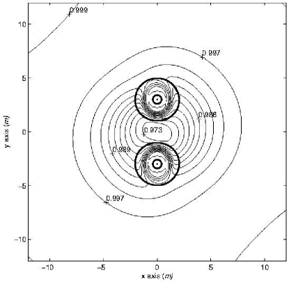
Figure 14: Conformal factor $\phi$ for two instantaneously stationary holes separated by $6m$ with spin parameter $a=0.5$. The spins are parallel and pointed out of the page. Compare to Fig. 10. Also notice the boundary effect on the outermost contour, labeled $0.999$.

Figure 15: Conformal factor $\phi$ for the same configuration as Fig. 14 except the spins are anti-parallel: the the spin of the hole at $(0,-3,0)$ points into the page.

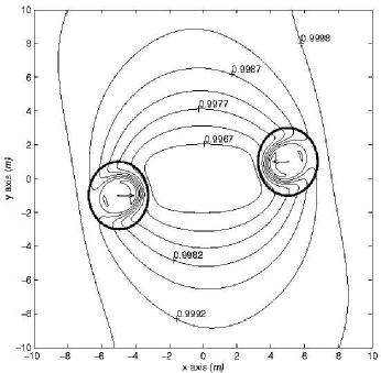
Figure 16: $\phi$ for a grazing collision between two equal mass, non-spinning holes. The holes are centered at $y=\pm 1m$ and boosted toward each other with $v_{x}=\mp 0.5c$, respectively.

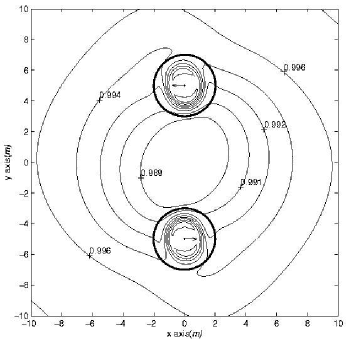
Figure 17: $\phi$ for two non-spinning holes boosted perpendicularly to their separation. The holes are separated by $10m$ and boosted with $v_{x}=\pm 0.196$, giving the system a background angular momentum of $\tilde{J}^{ADM}_{12}=2.0m^{2}$. The calculated $J^{ADM}_{12}=1.91m^{2}$ and $M_{ADM}=1.970m^{2}$. The Newtonian data correspond to an elliptic orbit at apastron.

Other derived quantities also show convergence: Fig. 12 shows the ADM mass $M_{{\rm ADM}}$ for two nonspinning black holes at $6m$ separation, and different resolutions. The fit is

$$M_{ADM}=\left(1.941+0.067\left(\frac{\Delta x}{m}\right)-0.422\left(\frac{\Delta x}{m}\right)^{2}\right)m.$$ (94)

showing good second order convergence. The angular momentum calculation is less robust, but exhibits approximately first order convergence. The fit to Figure 13, which shows $J^{ADM}$ for two nonspinning holes with orbital angular momentum, gives:

$$J^{ADM}_{12}=\left(1.837-0.121\left(\frac{\Delta x}{m}\right)+0.237\left(\frac{\Delta x}{m}\right)^{2}\right)\epsilon_{12}m^{2}.$$ (95)

Compare this to the angular momentum computed for the background: $\tilde{J}^{ADM}_{12}=2.0m^{2}$.

V.2 Physics Results

The small computational domain does not negate the utility of these solutions as initial data for the time-dependent Einstein equations. For instance, Figures 16 and 17 show data for grazing and elliptical orbits. They are currently being incorporated into the Texas binary black hole evolution code. While the small domains do mean that that our data do not represent the best asymptotically flat results available from this method, we can still verify some of the qualitative analytical predictions of the previous section. In particular, Figures 10, 14, and 15 show the conformal factor $\phi$ for holes instantaneously at rest at a separation of $6m$. In Figure 10 they are non-spinning; in Figures 14 and 15, each has Kerr parameter $a=0.5m$. In one case (Fig. 14) the spins are aligned; in the other (Fig. 15) they are antialigned. Table 4 gives the values of the apparent horizon area of each hole, the ADM mass, and the binding energy fraction for these configurations. The binding energy is consistent with the analytic estimates of Wald WaldPRD in Section IV.3.

Wald’s computation of the binding energy for spinning holes, Eq. (92), gives for parallel or antiparallel spins orthogonal to the separation (as in our computational models):

$${E_{b}}=-\left(\frac{mm^{\prime}}{\ell}+\frac{\vec{S}\cdot\vec{S^{\prime}}}{\ell^{3}}\right)$$ (96)

with oppositely directed spins showing less binding energy. For our $S=0.5~{}m^{2}$, $\ell=6~{}m$ configuration, this is a change of order ${\rm O}(2\times 10^{-3})$ between the parallel and the antiparallel cases. For the spinning cases we compute a change in binding energy between parallel and antiparallel spins of roughly half that, with the correct sign. This rough correspondence to the analytic result is suggestive. However, the nonspinning case deviates from the expectation that its binding energy should be between that of the spinning cases. Based on the scatter in the binding energies shown here, we estimate that we have achieved about $3\%$ accuracy in the binding energy. With the accuracy of our solution and the size of our domain, we are unable to present a clearer dependence of binding energy on spin.

	$A^{{\dagger}}_{AH}$	$M_{ADM}$	$M^{{\dagger}}_{AH}$	Binding Energy
Parallel Spin	53.20	1.973	1.065	-0.157 = -0.147 $\times M_{AH}$
Antiparallel Spin	53.17	1.974	1.065	-0.156 = -0.146 $\times M_{AH}$
Zero Spin	57.10	1.980	1.066	-0.151 = -0.142 $\times M_{AH}$

Table 4: $M_{ADM}$, $A_{AH}$ and associated quantities calculated for two holes with $m=1.0$ on a grid $(24~{}m)^{3}$ with resolution $\Delta x=m/8$.
^†: Quantity for a single hole.

VI Outlook

To an extent, the difficulty in setting data will become less relevant, as good evolutions are eventually achieved. Then data can be set for initial configurations with very large separation, and the subsequent evolution will tell us the future dynamics. In the shorter term, the iBBH program of Thorne and collaborators Brady will give us an indication of the evolution of the black hole parameters in the inspiral, and will allow a closer identification of the corresponding initial data sequence. To point out a couple of additional physical effects, note that, besides the historical component associated with a lagging tidal distortion, there is the familiar fact that most data setting methods are incapable of accounting for the previously emitted gravitational radiation. One can then expect that data describing hyperbolic encounters will be more accurate than data sets describing circular motion. This is because, in hyperbolic encounters, which are set as distant initial configurations, the radiation is more planar, and confined to near each hole. The radiation should then both be better defined, and should have less effect on the subsequent evolution than in the more distorted orbiting data set. In any case, the understanding of these problems is extremely significant in understanding the physical content of the configurations we must solve to provide waveforms for the new generation of gravitational wave detectors. For more accurate computational results, we are undertaking a both multigrid approach Klasky , and a spectral approach Pfeiffer2 ; GGB1 and expect to have extended results soon comparable to those of Pfeiffer2 ; Kidder . An ultimate goal of such a solver is to be able to carry out elliptic solutions at every integration time step, to enable fully constrained evolutions.

References

- (1) G. B. Cook, Phys. Rev. D50, 5025 (1994).
- (2) H. P. Pfeiffer, S. A. Teukolsky and G. B. Cook Phys. Rev. D62, 104018 (2000).
- (3) T. Baumgarte Phys. Rev. D62, 024018 (2000).
- (4) E. Gourgoulhon, P. Grandclement and S. Bonazzola, Phys. Rev. D65, 044020 (2002).
- (5) P. Grandclement, E. Gourgoulhon and S. Bonazzola, Phys. Rev. D65, 044021 (2002), and references therein.
- (6) E. Gourgoulhon, P. Grandclement and S. Bonazzola, Int. J. Mod. Phys. A17 2689–94 (2002).
- (7) G. B. Cook Phys. Rev. D65 084003 (2002).
- (8) H. P. Pfeiffer, G. B. Cook, and S. A. Teukolsky Phys. Rev. D66 024047 (2002).
- (9) G. B. Cook, Living Rev. Rel. 3, 5 (2000).
- (10) P. Peters and J. Matthews, Phys. Rev. 131,435 (1963).
- (11) T. Mora and C. Will, Phys. Rev. D66, 101501 (2002).
- (12) D. Shoemaker, M. F. Huq and R. A. Matzner Phys. Rev. D62, 124005 (2000).
- (13) M. F. Huq, M. Choptuik and R. A. Matzner, Phys. Rev. D66, 084024 (2002). [arXiv:gr-qc/0002076].
- (14) O. Dreyer, B. Krishnan, E. Schnetter, and D. Shoemaker, Phys. Rev. D67, 024018 (2003), and references therein.
- (15) Scott A. Caveny, PhD Dissertation, University of Texas at Austin (2002).
- (16) Scott A. Caveny, Matthew Anderson and Richard A. Matzner “Tracking Black Holes in Numerical Relativity”, submitted to Phys. Rev. (2003). [arXiv:gr-qc/0303099].
- (17) R. Arnowitt, S. Deser, and C. Misner in Witten, Gravitation, an Introduction to Current Research (Wiley, New York 1962).
- (18) J. York and T. Piran “The Initial Value Problem and Beyond”, Spacetime and Geometry: The Alfred Schild Lectures, R. Matzner and L. Shepley Eds. University of Texas Press, Austin, Texas. (1982); G. Cook, “Initial Data for the Two-Body Problem of General Relativity”, Ph.D. Dissertation, The University of North Carolina at Chapel Hill (1990).
- (19) N. Ó. Murchadha and J. W. York, Jr., Phys. Rev. D10, 428 (1974); N. Ó. Murchadha and J. W. York, Jr., Phys. Rev. D10, 437 (1974); N. Ó. Murchadha and J. W. York, Jr., Gen. Relativ. Gravit. 7 257 (1976).
- (20) J. W. York, Jr., Phys. Rev. Lett. 82, 1350 (1999).
- (21) J. R. Wilson and G. J. Mathews, Phys. Rev. Lett. 75, 4161 (1995); J. R. Wilson and G. J. Mathews, and P. Marronetti, Phys. Rev. D54, 1317 (1996)
- (22) J. Bowen and J. W. York, Phys. Rev. D21, 2047 (1980).
- (23) A. Garat and R. H. Price, Phys. Rev. D61, 124011 (2000) [arXiv:gr-qc/0002013].
- (24) N. Jansen, P. Diener, A. Khokhlov and I. Novikov, “Local and global properties of conformally flat initial data for black hole collisions,” Class. Quant. Grav. 20 51 (2003) [arXiv:gr-qc/0103109].
- (25) R. Matzner, M. F. Huq and D. Shoemaker, Phys. Rev. D59, 024015 (1999)[arXiv:gr-qc/9805023].
- (26) R. Kerr and A. Schild, “Some Algebraically Degenerate Solutions of Einstein’s Gravitational Field Equations,” in Applications of Nonlinear Partial Differential Equations in Mathematical Physics, Proc. of Symposia B Applied Math., Vol XVII (1965); “A New Class of Solutions of the Einstein Field Equations”, Atti del Congresso Sulla Relitivita Generale: Problemi Dell’Energia E Onde Gravitazionala G. Barbera, Ed. (1965).
- (27) C. W. Misner, K. S. Thorne, and J. A. Wheeler, Gravitation (W.H. Freeman, New York, 1970).
- (28) P. Marronetti, M. Huq, P. Laguna, L. Lehner, R. Matzner and D. Shoemaker, Phys. Rev. D62, 024017 (2000) [gr-qc/0001077].
- (29) P. Marronetti and R. A. Matzner Phys. Rev. Lett. 85 5500 (2000).
- (30) R. Wald, General Relativity (University of Chicago Press, Chicago, 1984).
- (31) For consistency of notation we use the superscript “ADM” to decorate the angular momentum . We are not certain where the formula (40) was first written. It does not appear in ADM . Expressions equivalent to it appear in Weinberg and in MTW , and were promulgated in notes by Misner (unpublished) in the mid-60s, arising from the long history of conservation law/pseudo-tensor studies in General Relativity. The form here was taken from Wald ; see also the very thorough development in Brown . Further, objections have been raised to our use of the symbol , rather than in Eq. (38). For a moving source, Eq. (38) would yield times the result for the same source not moving (a calculation facilitated by the Kerr-Schild structure); see the discussion around Eq. (43) below. We urge the reader to carefully follow our notation.
- (32) S. Weinberg, Gravitation and Cosmology (Wiley and Sons, New York, 1972)
- (33) J. D. Brown and J. W. York, Phys. Rev. D47, 1407 (1993).
- (34) Spatial components of angular momentum (e.g. spin) perpendicular to the motion transform with one power of and stay perpendicular to the motion. The orbital angular momentum also contains one power of in . Hence contains one power of . See Landau and Lifshitz, Classical Theory of Fields revised second edition, (Pergamon Press, Oxford, 1962), p. 46.
- (35) D. Brill and R. W. Lindquist Phys. Rev. 131 471 (1963).
- (36) This was apparently first noticed as a computational result; see A. Čadež, Ann. Phys. (NY) 83 449 (1974). Čadež considered both the Brill-Lindquist Brill and Misner Misner data. For Brill-Lindquist data the apparent horizon areas are easy to compute to , because the lowest order effect of the distant hole on the local one is a constant, isotropic addition to the local value of the conformal factor.
- (37) C. Misner, Phys. Rev. 118, 1110 (1960).
- (38) R. H. Price and J. T. Whelan, Phys. Rev. Lett. 87, 231101 (2001) [arXiv:gr-qc/0107029].
- (39) Black Holes, the Membrane Paradigm, K. S. Thorne, R. H. Price, D .A. Macdonald, editors. (Yale University Press, New Haven, 1986), Section VIII B 1.
- (40) S. A. Teukolsky, PhD Dissertation, California Institute of Technology, (1973).
- (41) R. Wald, Phys. Rev. D6, 406 (1972).
- (42) S. Dain Phys. Rev.D66 084019 (2002).
- (43) W. H. Press, S. A. Teukolsky, W. T. Vetterling, and B. P. Flannery, Numerical Recipies in Fortran, Second Edition (Cambridge University Press, Cambridge, 1992).
- (44) H. Pfeiffer L. Kidder, M. Scheel and S. A. Teukolsky [arXiv:gr-qc 0202096].
- (45) P. Brady, J. Creighton and K. S. Thorne, Phys. Rev. D58, 061501 (1998).
- (46) S. Klasky, PhD Dissertation, University of Texas at Austin, (1966).