Dynamical system approach to FRW models in higher-order gravity theories

Abstract

We study the late time evolution of positively curved FRW models with a scalar field which arises in the conformal frame of the $R+\alpha R^{2}$ theory. The resulted three-dimensional dynamical system has two equilibrium solutions corresponding to a de Sitter space and an ever expanding closed universe. We analyze the structure of the first equilibrium with the methods of the center manifold theory and, for the second equilibrium we apply the normal form theory to obtain a simplified system, which we analyze with special phase plane methods. It is shown that an initially expanding closed FRW spacetime avoids recollapse.

1 Introduction

A central question in relativistic cosmology is that of deciding about the past and future asymptotic states of cosmological models [1]. However, general relativity leads to singularities in the spacetimes of all known cosmological models with ordinary matter. Higher order curvature corrections in the gravitational action may rectify the problem and lead to cosmological models free from such pathologies, at the cost of diverging from a FRW behavior at late times [2]. There is a resurgence of interest in such theories which naturally arise in string-theoretic considerations (cf. brane models with Gauss-Bonett terms [3, 4, 5, 6]). An interesting feature of higher order theories is that inflation emerges in these theories in a most direct way. In one of the first inflationary models, proposed in 1980 by Starobinsky [7], inflation is due to the $R^{2}$ correction term in a gravitational Lagrangian $L=R+\alpha R^{2}$ where $\alpha$ is a constant. The dynamics of higher order cosmologies is closely related to scalar-field cosmologies in general relativity because of their conformal equivalence [8, 9]. There are certain limitations to this procedure related to the issue of physical reality of the two metrics involved [10] and to the fact that the conformal transformation may fail to be regular at all points of the spacetime. Nevertheless, it is practically useful and investigations in the conformal frame have given some interesting results, e.g. the cosmic no-hair theorem in quadratic cosmologies [11, 12].

Most of the studies of scalar-field cosmologies with the dynamical systems methods are restricted to FRW models (see for example [13, 14] and references therein), although there are important investigations in spatially homogeneous Bianchi cosmologies with an exponential potential [15]. In particular, for flat FRW models with a scalar field there are some general results which do not rely on the particular properties of the potential [16, 17]. However, the situation is more delicate for positively curved FRW models with a scalar field having a potential with a zero local minimum. The main problem which confronts us is the following: Can a closed universe filled with ordinary matter and a scalar field avoid recollapse?

In this paper we investigate the evolution of positively curved FRW models with a scalar field having the potential which arises in the conformal frame of the $R+\alpha R^{2}$ theory in vacuum [8, 11]. The motivation for this choice is presented in Section III. The dimension of the dynamical systems involved in such models is greater than two and the usual methods of phase plane analysis cannot be applied. In particular, for nonhyperbolic equilibrium points the linearization theorem does not yield any information about the stability of the equilibria and therefore, more powerful methods are needed. The center manifold theorem shows that the qualitative behavior in a neighborhood of a nonhyperbolic equilibrium point $\mathbf{q}$ is determined by its behavior on the center manifold near $\mathbf{q\,.}$ Since the dimension of the center manifold is generally smaller than the dimension of the dynamical system, this greatly simplifies the problem. The other general method for simplifying the dynamical system is the normal form theory, which consists in a nonlinear coordinate transformation that allows to simplify the nonlinear part of the system. Both methods are used in Sections III and IV respectively.

The plan of the paper is as follows. In the next Section we write down the field equations assuming an arbitrary potential, as a constrained four-dimensional dynamical system. In Section III, we use the constraint equation to reduce the dimension of the system to three and after a suitable change of variables we find the equilibrium points of the system and discuss the physical meaning of these particular solutions. In particular we show using the methods of the center manifold theory that, the equilibrium corresponding to the de Sitter solution is asymptotically unstable. In Section IV we find the so-called normal form of the dynamical system, which greatly simplifies the problem, since two of the equations decouple. We study the qualitative behavior of the resulted two-dimensional system and analyze the late time evolution of the model. We show that an initially expanding universe avoids recollapse. In Section V we apply the same techniques to flat FRW spaces filled with a barotropic fluid in the conformal frame of the $R+\alpha R^{2}$ theory and study the detailed evolution of the models.

2 Scalar-field cosmologies

In general relativity the evolution of FRW models with a scalar field (ordinary matter is described by a perfect fluid with energy density $\rho$ and pressure $p$) are governed by the Friedmann equation,

$$\left(\frac{\dot{a}}{a}\right)^{2}+\frac{k}{a^{2}}=\frac{1}{3}\left(\rho+\frac{1}{2}\dot{\phi}^{2}+V\left(\phi\right)\right),$$ (1)

the Raychaudhuri equation,

$$\frac{\ddot{a}}{a}=-\frac{1}{6}\left(\rho+3p+2\dot{\phi}^{2}-2V\right),$$ (2)

the equation of motion of the scalar field,

$$\ddot{\phi}+3\frac{\dot{a}}{a}\dot{\phi}+V^{\prime}\left(\phi\right)=0$$ (3)

and the conservation equation,

$$\dot{\rho}+3\left(\rho+p\right)\frac{\dot{a}}{a}=0.$$ (4)

We adopt the metric and curvature conventions of Ref. [1]. Here, $a\left(t\right)$ is the scale factor, an overdot denotes differentiation with respect to time $t$ and units have been chosen so that $c=1=8\pi G.$

From Eqs. (1)-(4) we see that the state $\left(a,\dot{a},\rho,\phi,\dot{\phi}\right)\in\mathbb{R}^{5}$ of the system lies on the hypersurface defined by the constraint, (1), and the remaining field equations can be written as a five-dimensional dynamical system. In vacuum, $\rho=0,$ the dimension of the dynamical system reduces to four.

In the literature of scalar-field cosmologies the exponential potential function viz. $V\left(\phi\right)=V_{0}e^{-\lambda\phi}$, is the most popular not only because of the variety of alternative theories of gravity which predict exponential potentials, but also due to the fact that this potential has the nice property that $V^{\prime}\propto V$ which allows the introduction of normalized variables according to the formalism of Wainwright et al [1]. In flat, $k=0$ FRW models for example with a scalar field having an exponential potential, introducing the variables $x\sim\dot{\phi}/H,\;y\sim\sqrt{V}/H$ and the time coordinate $\tau=\ln\left(a/a_{0}\right)$, enables the evolution equations to be written as a two-dimensional dynamical system (cf. [18]) and in more general homogeneous cosmologies associated with a scalar field, the dimension of the dynamical system reduces by one if the potential function is exponential.

If we set $\dot{\phi}=y,\,\;\dot{a}/a=H$ the evolution equations (2)-(4) in vacuum become

$$\dot{a} =Ha$$

$$\dot{\phi} =y,$$

$$\dot{y} =-3Hy-V^{\prime}\left(\phi\right),$$

$$\dot{H} =-\frac{1}{2}y^{2}+k/a^{2},$$ (5)

subject to the constraint

$$3H^{2}+3k/a^{2}=\frac{1}{2}y^{2}+V\left(\phi\right).$$ (6)

Therefore, the phase space of the dynamical system (5) is the set

$$\left\{\left(a,\phi,y,H\right)\in\mathbb{R}^{4}:3H^{2}+3k/a^{2}=\frac{1}{2}y^{2}+V\left(\phi\right)\right\}.$$

3 Curved FRW in $R+\alpha R^{2}$ theory: Equilibria

In the remainder of the paper we assume that the potential function of the scalar field is

$$V\left(\phi\right)=V_{\infty}\left(1-e^{-\sqrt{2/3}\phi}\right)^{2}$$ (7)

which arises in the conformal frame of the $R+\alpha R^{2}$ theory [8, 11]. This potential has a long and flat plateau. For large values of $\phi,$ the potential, $V,$ is almost constant, $V_{\infty}=\lim_{\phi\rightarrow+\infty}V\left(\phi\right),$ thus $V$ has the general properties for inflation to commence. In [12] it was proved a cosmic no-hair theorem, i.e. Bianchi models with ordinary matter satisfying the strong energy condition and a scalar field with potential (7), asymptotically isotopize. According to this picture, the universe started in a homogeneous state and during inflation it had enough time to isotropize.

In order to reduce the dimension of the dynamical system (5) we use the constraint (6) to eliminate $a.$ The evolution equations become

$$\dot{\phi} =y,$$

$$\dot{y} =-3Hy-V^{\prime}\left(\phi\right),$$

$$\dot{H} =-H^{2}-\frac{1}{3}y^{2}+\frac{1}{3}V\left(\phi\right).$$ (8)

Linearization of (8) near the equilibrium point $\left(0,0,0\right)$ shows that the Jacobian matrix at that point has one zero and two purely imaginary eigenvalues. Consequently the Hartman-Grobman theorem does not apply. Therefore, we cannot draw any conclusions about the stability of the equilibrium from an examination of the Jacobian.

We simplify the system by rescaling the variables by the equations

$$\phi \rightarrow\sqrt{2/3}\phi,$$

$$y \rightarrow\sqrt{4V_{\infty}/3}\,\,y,$$

$$H \rightarrow\frac{\sqrt{2V_{\infty}}}{3}H,$$

$$t \rightarrow\frac{1}{\sqrt{2V_{\infty}}}t.$$

In order to take account of the equilibrium point corresponding to the point at “infinity” and to remove the transcendental functions, it is convenient to introduce the variable $u$ defined by

$$u:=e^{-\phi},$$ (9)

to obtain finally

$$\dot{u} =-uy,$$

$$\dot{y} =-Hy-u\left(1-u\right),$$

$$\dot{H} =-\frac{1}{3}H^{2}-\frac{2}{3}y^{2}+\frac{1}{2}\left(1-u\right)^{2}.$$ (10)

Note that under the transformation (9), the resulted three-dimensional dynamical system (10) is quadratic. In view of (6) we have $3H^{2}-\frac{1}{2}y^{2}-V\left(\phi\right)>0,$ hence, the phase space of the system (10) is the set

$$\Sigma:=\left\{\left(u,y,H\right)\in\mathbb{R}^{3}:H^{2}-y^{2}-\frac{3}{2}\left(1-u\right)^{2}>0\right\}.$$ (11)

The equilibrium points of (10) are:

A: $\left(u=1,y=0,H=0\right).$ This corresponds to the limiting state of an ever-expanding universe with $H\rightarrow 0$ while the scalar field approaches the minimum of the potential and the scale factor goes to infinity. Equality in (11) which arises from the flat, $k=0,$ case defines a set on the boundary of $\Sigma.$ We conclude that the point A which corresponds to the Minkowski solution, is located on this boundary. The detailed structure of this equilibrium will be analyzed in the next Section.

B: $\left(u=0,y=\pm\sqrt{3}/2,H=0\right).$ These lie outside of the phase space and, therefore, are unphysical.

C: $\left(u=0,y=0,H=\pm\sqrt{3/2}\right).$ In the next Section we show that only the point with the $+$ sign can be approached by a trajectory starting with a $H>0.$ It corresponds to the de Sitter universe with a cosmological constant equal to $\sqrt{V_{\infty}}$. Regarding the stability of this equilibrium, it is easy to see that the Jacobian matrix of (10) at $\mathbf{q}=\left(0,0,\sqrt{3/2}\right)$ has one zero and two negative eigenvalues. The center manifold theorem implies that there exists a local 2-dimensional stable manifold through $\mathbf{q}$ (see for example [19]). That means that all trajectories asymptotically approaching $\mathbf{q}$ as $t\rightarrow\infty,$ lie on a 2-dimensional invariant manifold. Since $\mathbf{q}$ is a nonhyperbolic fixed point, the topology of the flow near $\mathbf{q}$ is nontrivial and is characterized by a one-dimensional local center manifold intersecting $\mathbf{q}.$ In the Appendix we prove the following result.

Proposition 1

The equilibrium point $\mathbf{q}=\left(0,0,\sqrt{3/2}\right)$ of (10) is locally asymptotically unstable.

4 Late time evolution

It is easy to see that at the equilibrium point, $\left(u=1,y=0,H=0\right),$ the eigenvalues of the Jacobian of (10) are $\pm i,0$ and therefore, we cannot infer about the stability of the equilibrium. Nevertheless, it is the most interesting case, because in all other equilibria the scalar field reaches the flat plateau, which is impossible if we restrict ourselves to initial values of $H$ smaller than $\sqrt{V_{\infty}}$. The study of the qualitative behavior of a dynamical system near a nonhyperbolic equilibrium point is difficult even in two dimensions. We find the so-called normal form (cf. [19] for a brief introduction) of the system (10) near the equilibrium point $\left(u=1,y=0,H=0\right).$ The idea of the normal form theory is the following: Given a dynamical system with equilibrium point at the origin, $\mathbf{\dot{x}}=A\mathbf{x}+\mathbf{f}\left(\mathbf{x}\right),$ where $A$ is the Jordan form of the linear part and $\mathbf{f}\left(\mathbf{0}\right)=\mathbf{0}$, perform a non-linear transformation $\mathbf{x}\rightarrow\mathbf{x}+\mathbf{h}\left(\mathbf{x}\right),$ where $\mathbf{h}\left(\mathbf{x}\right)=O\left(\left|\mathbf{x}\right|^{2}\right)$ as $\left|\mathbf{x}\right|\rightarrow 0,$ such that the system becomes “as simple as possible”.

To write the system in a form suitable for the application of the normal form theory, we shift the fixed point to $\left(0,0,0\right)$ by setting $x=u-1$ and the system becomes

$$\dot{x} =-y-xy,$$

$$\dot{y} =x+x^{2}-Hy,$$

$$\dot{H} =\frac{1}{2}x^{2}-\frac{2}{3}y^{2}-\frac{1}{3}H^{2}.$$ (12)

We now perform the non-linear transformation

$$x \rightarrow x-y^{2}+\frac{1}{4}Hy,$$

$$y \rightarrow y+xy+\frac{1}{4}Hx,$$

$$H \rightarrow H+\frac{7}{12}xy,$$

and keeping only terms up to second order we obtain the system

$$\dot{x} =-y-\frac{1}{2}Hx,$$

$$\dot{y} =x-\frac{1}{2}Hy,$$

$$\dot{H} =-\frac{1}{12}\left(x^{2}+y^{2}\right)-\frac{1}{3}H^{2}.$$ (13)

Note that the results are valid only near the origin.

Passing to cylindrical coordinates $\left(x=r\cos\theta,y=r\sin\theta,H=H\right),$ we have

$$\dot{r} =-\frac{1}{2}rH,\;$$

$$\;\dot{\theta} =1,$$

$$\dot{H} =-\frac{1}{12}r^{2}-\frac{1}{3}H^{2}\;.$$ (14)

We note that the $\theta$ dependence of the vector field has been eliminated, so that we can study the system on the $r-H$ plane. The equation $\dot{\theta}=1$ means that the trajectory in the $x-y$ plane spirals with angular velocity $1.$ It is convenient to rescale the variables by

$$r\rightarrow 6r,\;\;H\rightarrow 3H$$ (15)

so that the projection of (14) on the $r-H$ plane is

$$\dot{r} =-\frac{3}{2}rH,\;$$

$$\dot{H} =-r^{2}-H^{2}\;.$$ (16)

This system belongs to a family of systems studied in 1974 by Takens [20].

It is easy to obtain the phase portrait of (16) via numerical integration. However, we can analyze the qualitative behavior of the trajectories using theoretical arguments. Firstly, (16) is invariant under the transformation $t\rightarrow-t,$ $H\rightarrow-H$ (which implies that all trajectories are symmetric with respect to the $r$ axis) and the line $r=0$ is invariant. Secondly, the system (16) has invariant lines $H=cr$. To see this, write

$$\frac{dH}{dr}=c=\frac{-r^{2}-c^{2}r^{2}\;}{-\frac{3}{2}cr^{2}}=\frac{-1-c^{2}\;}{-\frac{3}{2}c}\Rightarrow c=\pm\sqrt{2}.$$ (17)

Taking the dot product of the vector field $\left(-\frac{3}{2}rH,-r^{2}-H^{2}\right)^{\perp}$ with the radial vector $\left(r,H\right)^{\perp}$ along the line $H=cr$ we find that it is negative for $H>0$ and positive for $H<0.$ Therefore, the direction of the flow along $H=cr$ in the first quadrant is towards the origin and goes away from the origin in the second quadrant. Note that $H$ is always decreasing along the orbits while $r$ is decreasing in the first quadrant. Since no trajectory can cross the line $H=cr,$ all trajectories starting above this line, approach the origin asymptotically. On any orbit starting in the first quadrant below the line $H=cr,$ $H$ becomes zero at some time and the trajectory crosses vertically the $r-$axis. Once the trajectory enters the second quadrant, $r$ increases and $H$ decreases. The phase portrait is shown in Figure 1.

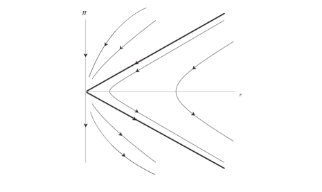
Figure 1: The phase portrait of (16). The invariant trajectories $H=\pm\sqrt{2}r$ are shown with thicker lines. For expanding models only trajectories above the line $H=\sqrt{6}r$ belong to the phase space of the system.

At first sight, it seems probable that an initially expanding universe may recollapse. However, the phase space of the dynamical system (16) is not the whole $r-H$ plane, because of the constraint (11), which in terms of the variables (15) becomes

$$H^{2}>6r^{2}.$$ (18)

Therefore, for an expanding universe we should consider only trajectories starting above the line $H=\sqrt{6}r$ and according to the previous discussion all these trajectories asymptotically approach the origin.

We now turn to the relation of the dynamics in the $r-H$ plane to the full three-dimensional system (14), or the equivalent (13) in Cartesian coordinates. Any trajectory spirals clockwise in the $x-y$ plane while both $H$ and $x^{2}+y^{2}$ are decreasing. In physical terms this means that the scalar field oscillates around the minimum of the potential with a decreasing amplitude, $H$ is always decreasing and, in view of (6), the curvature decreases. A typical trajectory of (13) is shown in Figure 2.

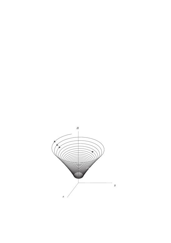
Figure 2: Trajectories of the full three-dimensional system spiral approaching the origin.

5 Comment on Flat FRW models

Consider a flat FRW model containing a barotropic fluid with an equation of state $p=(\gamma-1)\rho,$ where $0\leq\gamma\leq 2,$ and a scalar field having the potential (7). Then the system (2)-(4) reduces again to a four-dimensional dynamical system, namely

$$\dot{\phi} =y,$$

$$\dot{y} =-3Hy-V^{\prime}\left(\phi\right),$$

$$\dot{\rho} =-3\gamma\rho H,$$

$$\dot{H} =-\frac{1}{2}y^{2}-\frac{\gamma}{2}\rho,$$ (19)

subject to the constraint

$$3H^{2}=\rho+\frac{1}{2}y^{2}+V\left(\phi\right).$$ (20)

In contrast to (5d), the forth of (19) implies that $H$ is always decreasing. If we use the constraint (20) to eliminate $\rho,$ the evolution equations become

$$\dot{\phi} =y,$$

$$\dot{y} =-3Hy-V^{\prime}\left(\phi\right),$$

$$\dot{H} =-\frac{3\gamma}{2}H^{2}-\frac{2-\gamma}{4}y^{2}+\frac{\gamma}{2}V\left(\phi\right).$$ (21)

We see that the structure of (21) describing a flat FRW model with a perfect fluid and a scalar field, apart from being parameter dependent, has a striking similarity to the dynamical system (8) for the vacuum positively curved FRW with a scalar field. Proceeding as in Section IV, we end up with the following system in cylindrical coordinates

$$\dot{r} =-\frac{1}{2}rH,\;$$

$$\;\dot{\theta} =1,$$

$$\dot{H} =\frac{5\gamma-4}{8}r^{2}-\frac{\gamma}{2}H^{2}\;.$$ (22)

Although the system (22) depends only on one parameter, it is convenient to rescale the variables by

$$r\rightarrow\lambda r,\;\;H\rightarrow\mu H$$ (23)

with

$$\mu=\frac{2}{\gamma},\;\;\lambda=\sqrt{\left|\frac{16}{\gamma\left(5\gamma-4\right)}\right|},$$

so that the projection of (22) on the $r-H$ plane is

$$\dot{r} =-\frac{1}{\gamma}rH,\;$$

$$\dot{H} =br^{2}-H^{2}\;,$$ (24)

where

$$b=+1\;\mathrm{for\;}\gamma>4/5,\;\;b=-1\;\mathrm{for\;}\gamma<4/5.$$

Note that (24) has a first integral, viz.

$$I\left(r,H\right)=-\frac{1}{2\gamma}r^{-2\gamma}\left(\frac{br^{2}}{1-1/\gamma}-H^{2}\right).$$ (25)

In fact, it is straightforward to verify that $\left(\partial I/\partial r\right)\dot{r}+\left(\partial I/\partial H\right)\dot{H}=0$ along the solution curves of (24). The level curves of $I$ are the trajectories of the system (cf. Figure 3).

Invariant lines $H=cr$ exist for certain values of the parameter $\gamma.$ We find (cf. (17))

$$c=\pm\sqrt{\frac{b}{1-1/\gamma}}.$$

Case I. For $b=+1,$ invariant lines exists if $\gamma>1.$ We find that the direction of the flow along $H=cr$ in the first quadrant is towards the origin and goes away from the origin in the second quadrant. Note that in the first quadrant $r$ is decreasing along the orbits and that $\dot{H}$ vanishes along the line $H=r,$ which lies below the invariant line $H=cr.$ It can be shown that in the first quadrant a level curve of $I\left(r,H\right)$ may intersect the line $H=r$ only once (it is sufficient to consider the level curve passing through an arbitrary point $\left(r_{1},0\right)$ and compute the $r$ coordinate at the intersection with the line $H=r$). We conclude that once a trajectory crosses the line $H=r,$ it is trapped between the lines $H=r$ and $H=cr$ and, since $\dot{r}<0,$ it approaches the origin asymptotically.

Case II. $b=+1$ and $4/5<\gamma<1.$ There are no invariant lines. Similar arguments as in case I, yield the phase portrait shown in Fig.3.

Case III. $\gamma<4/5$ $\left(\Rightarrow b=-1\right).$ The analysis is exactly the same as in Section IV.

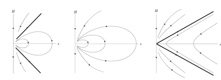
Figure 3: The phase portrait of (24) for $1<\gamma<2,$ $4/5<\gamma<1$ and $0<\gamma<4/5$ respectivelly.

In all cases we must remember that the phase space of the dynamical system (24) is not the whole $r-H$ plane, because of the constraint (11), which in terms of the variables (23) reads

$$H^{2}>\frac{6\gamma}{\left|5\gamma-4\right|}r^{2}.$$ (26)

Therefore, for an expanding universe, we should consider only trajectories starting above the line $H=\sqrt{6\gamma/\left|5\gamma-4\right|}r,$ which in case III lies always above the line $H=cr$ and according to the previous discussion all these trajectories asymptotically approach the origin.

We conclude that, in the conformal frame of the $R+aR^{2}$ theory, an initially expanding flat universe with a barotropic fluid as matter source remains ever-expanding and eventually the quadratic curvature corrections become negligible. This result, established by stability analysis, is in accordance with the general properties of all flat FRW models with a scalar field having a potential with a unique zero minimum [17].

6 Discussion

We have analyzed the qualitative behavior of a positively curved FRW model containing a scalar field with the potential (7). This model is conformally equivalent to the positively curved FRW spacetime in the simplest higher order gravity theory, namely the $R+\alpha R^{2}$ theory. We have shown that an initially expanding closed universe avoids recollapse provided that the initial value of $H$ is less than $\sqrt{V_{\infty}}.$ This result should be compared to a counterexample of the closed universe recollapse conjecture (cf. [21] where it is shown that initially expanding vacuum diagonal Bianchi IX models in purely quadratic gravity are ever-expanding). It should be of interest to investigate if a closed FRW universe filled with ordinary matter satisfying the usual energy conditions and a scalar field with the potential (7) can avoid recollapse. This is equivalent to the analysis of the qualitative behavior of the full five-dimensional system (2)-(4). A partial answer to this question for an arbitrary non-negative potential having a unique minimum $V\left(0\right)=0$ is given in [17].

Acknowledgments I thank P.G.L. Leach and S. Cotsakis for fruitful discussions during the preparation of this work. I wish to thank an anonymous referee for useful suggestions, especially for pointing me out the remarks regarding the equilibrium A after eq. (11).

Appendix A Proof of Proposition 1

In order to determine the local center manifold of (10) at $\mathbf{q},$ we have to transform the system into a form suitable for the application of the center manifold theorem. The procedure is fairly systematic and will be accomplished in the following steps.

1. The Jacobian of (10) at $\mathbf{q}=\left(0,0,\sqrt{3/2}\right)$ has eigenvalues $0,-\sqrt{2/3}$ and $-\sqrt{3/2}$ with corresponding eigenvectors $\left(-\sqrt{2/3},2/3,1\right)^{{}^{\top}},$ $\left(0,0,1\right)^{{}^{\top}}$ and $\left(0,1,0\right)^{{}^{\top}}.$ Let $T$ be the matrix having as columns these eigenvectors. We shift the fixed point to $\left(0,0,0\right)$ by setting $\widetilde{H}=H-\sqrt{3/2}$ and write (10) in vector notation as

$$\mathbf{\dot{z}}=A\mathbf{z}+\mathbf{F}\left(\mathbf{z}\right),$$ (A.1)

where $A$ is the linear part of the vector field and $\mathbf{F}\left(\mathbf{0}\right)=\mathbf{0}$.

2. Using the matrix $T$ which transforms the linear part of the vector field into Jordan canonical form, we define new variables, $\left(x,y_{1},y_{2}\right)\equiv\mathbf{x}$, by the equations

$$u =-\sqrt{\frac{2}{3}}x,$$

$$y =\frac{2}{3}x+y_{2},$$

$$\widetilde{H} =x+y_{1},$$

or in vector notation $\mathbf{z}=T\mathbf{x},$ so that (A.1) becomes

$$\mathbf{\dot{x}}=T^{-1}AT\mathbf{x}+T^{-1}\mathbf{F}\left(T\mathbf{x}\right).$$

Denoting the canonical form of $A$ by $B$ we finally obtain the system

$$\mathbf{\dot{x}}=B\mathbf{x}+\mathbf{f}\left(\mathbf{x}\right),$$ (A.2)

where $\mathbf{f}\left(\mathbf{x}\right):=T^{-1}\mathbf{F}\left(T\mathbf{x}\right).$ In components system (A.2) is

$$\left(\begin{array}[c]{c}\dot{x}\\ \dot{y}_{1}\\ \dot{y}_{2}\end{array}\right) =\left(\begin{array}[c]{ccc}0&0&0\\ 0&-\sqrt{\frac{2}{3}}&0\\ 0&0&-\sqrt{\frac{3}{2}}\end{array}\right)\left(\begin{array}[c]{c}x\\ y_{1}\\ y_{2}\end{array}\right)$$ (A.12)

$$+\left(\begin{array}[c]{l}-\frac{2}{3}x^{2}-xy_{2}\\ \frac{10}{27}x^{2}-\frac{1}{3}y_{1}^{2}-\frac{2}{3}y_{2}^{2}-\frac{2}{3}xy_{1}+\frac{1}{9}xy_{2}\\ \frac{4}{9}x^{2}-\frac{2}{3}xy_{1}-\frac{1}{3}xy_{2}-y_{1}y_{2}\end{array}\right).$$ (A.16)

3. The system (A.16) is written in diagonal form

$$\dot{x} =Cx+f\left(x,\mathbf{y}\right)$$

$$\mathbf{\dot{y}} =P\mathbf{y}+\mathbf{g}\left(x,\mathbf{y}\right),$$ (A.17)

where $\left(x,\mathbf{y}\right)\in\mathbb{R}\times\mathbb{R}^{2},$ $C$ is the zero $1\times 1$ matrix, $P$ is a square matrix with negative eigenvalues and $f,\mathbf{g}$ vanish at $\mathbf{0}$ and have vanishing derivatives at $\mathbf{0.}$ The center manifold theorem asserts that there exists a 1-dimensional invariant local center manifold $W^{c}\left(\mathbf{0}\right)$ of (A.17) tangent to the center subspace (the $\mathbf{y}=\mathbf{0}$ space) at $\mathbf{0}.$ Moreover, $W^{c}\left(\mathbf{0}\right)$ can be represented as

$$W^{c}\left(\mathbf{0}\right)=\left\{\left(x,\mathbf{y}\right)\in\mathbb{R}\times\mathbb{R}^{2}:\mathbf{y}=\mathbf{h}\left(x\right),\;\left|x\right|<\delta\right\};\;\;\;\mathbf{h}\left(0\right)=0,\;D\mathbf{h}\left(0\right)=\mathbf{0},$$

for $\delta$ sufficiently small (cf. [19], p. 155). The restriction of (A.17) to the center manifold is

$$\dot{x}=Cx+f\left(x,\mathbf{h}\left(x\right)\right).$$ (A.18)

According to Theorem 3.2.2 in [22], if the origin $x=0$ of (A.18) is stable (resp. unstable) then the origin of (A.17) is also stable (resp. unstable). Therefore, we have to find the local center manifold, i.e., the problem reduces to the computation of $\mathbf{h}\left(x\right).$

4. Substituting $\mathbf{y}=\mathbf{h}\left(x\right)$ in the second component of (A.17) and using the chain rule, $\mathbf{\dot{y}}=D\mathbf{h}\left(x\right)\dot{x}$, one can show that the function $\mathbf{h}\left(x\right)$ that defines the local center manifold satisfies

$$D\mathbf{h}\left(x\right)\left[Cx+f\left(x,\mathbf{h}\left(x\right)\right)\right]-P\mathbf{h}\left(x\right)-\mathbf{g}\left(x,\mathbf{h}\left(x\right)\right)=0.$$ (A.19)

This condition allows for an approximation of $\mathbf{h}\left(x\right)$ by a Taylor series at $x=0.$ Since $\mathbf{h}\left(0\right)=0,D\mathbf{h}\left(0\right)=\mathbf{0},$ it is obvious that $\mathbf{h}\left(x\right)$ commences with quadratic terms. We substitute

$$\mathbf{h}\left(x\right)=:\left(\begin{array}[c]{c}h_{1}\left(x\right)\\ h_{2}\left(x\right)\end{array}\right)=\left(\begin{array}[c]{c}a_{1}x^{2}+a_{2}x^{3}+O\left(x^{4}\right)\\ b_{1}x^{2}+b_{2}x^{3}+O\left(x^{4}\right)\end{array}\right)$$

into (A.19) and set the coefficients of like powers of $x$ equal to zero to find the unknowns $a_{1},b_{1},...$.

5. Since $y_{1}$ is absent from the first of (A.16), we give only the result for $h_{2}\left(x\right).$ We find $b_{1}=\frac{4}{9}\sqrt{\frac{2}{3}},$ $b_{2}=\frac{4}{81}.$ Therefore, (A.18) yields

$$\dot{x}=-\frac{2}{3}x^{2}-\frac{4}{9}\sqrt{\frac{2}{3}}x^{3}-\frac{4}{81}x^{4}+O\left(x^{5}\right).$$ (A.20)

It is obvious that the origin $x=0$ of (A.20) is asymptotically unstable (saddle point). The theorem mentioned after (A.18) implies that the origin $\mathbf{x}=\mathbf{0}$ of the full three-dimensional system is unstable. This completes the proof.

References

- [1] J. Wainwright and G.F.R. Ellis, Dynamical Systems in Cosmology, (Cambridge University Press, 1997).
- [2] A.A. Ruzmaikin and T.V. Ruzmaikina, Sov. Phys. Lett. JETP 30, 372 (1970).
- [3] J.E. Lidsey, S. Nojiri and S.D. Odintsov, JHEP 0206, 026 (2002).
- [4] C. Charmousis and J.F. Dufaux, Class. Quant. Grav. 19, 4671 (2002).
- [5] S. Mukohyama, Phys. Rev. D65, 084036 (2002).
- [6] B. Abdesselam and N. Mohammedi, Phys. Rev. D65, 084018 (2002).
- [7] A. Starobinsky, Phys. Lett. 91B, 99 (1980).
- [8] J.D. Barrow and S. Cotsakis, Phys. Lett. B214, 515 (1988).
- [9] S. Gottlöber, V. Müller, H. Schmidt and A. Starobinsky, Int. J. Mod. Phys. D2, 257 (1992).
- [10] S. Cotsakis, Phys. Rev. D47, 1437 (1993); Erratum Phys. Rev. D49, 1145; S. Cotsakis, Phys. Rev. D52, 6199 (1995).
- [11] K. Maeda, Phys. Rev. D37, 858 (1988).
- [12] S. Cotsakis and J. Miritzis, Class. Quant. Grav. 15, 2795 (1998).
- [13] E. Gunzig et al, Class. Quant. Grav. 17, 1783 (2000).
- [14] A.A. Coley, gr-qc/9910074 (1999).
- [15] A.A. Coley, J. Ibáñez and R.J. van den Hoogen, J. Math. Phys. 38, 5256 (1997).
- [16] S. Foster, Class. Quant. Grav. 15, 3485 (1998).
- [17] J. Miritzis, Scalar-field cosmologies with an arbitrary potential, gr-qc/0303014 (2003).
- [18] E.J. Copeland, A.R. Liddle and D. Wands, Phys. Rev. D57, 4686 (1998).
- [19] L. Perko, Differential Equations and Dynamical Systems, (Springer-Verlag, 1991).
- [20] F. Takens, Publ. Math. IHES, 43, 47 (1974).
- [21] S. Cotsakis, G. Flessas, P.G.L. Leach and L. Querella, Grav.Cosmol. 6, 291 (2000).
- [22] J. Guckenheimer and P. Holmes, Nonlinear Oscillations, Dynamical Systems and Bifurcations of Vector Fields, (Springer-Verlag, New York, 1983).