Critical Collapse of the Massless Scalar Field in Axisymmetry

Abstract

We present results from a numerical study of critical gravitational collapse of axisymmetric distributions of massless scalar field energy. We find threshold behavior that can be described by the spherically symmetric critical solution with axisymmetric perturbations. However, we see indications of a growing, non-spherical mode about the spherically symmetric critical solution. The effect of this instability is that the small asymmetry present in what would otherwise be a spherically symmetric self-similar solution grows. This growth continues until a bifurcation occurs and two distinct regions form on the axis, each resembling the spherically symmetric self-similar solution. The existence of a non-spherical unstable mode is in conflict with previous perturbative results, and we therefore discuss whether such a mode exists in the continuum limit, or whether we are instead seeing a marginally stable mode that is rendered unstable by numerical approximation.

I Introduction

In this paper we present results from a numerical study of critical collapse of the massless scalar field in axisymmetry. In spherical symmetry, the threshold of black hole formation was first systematically explored in choptuik , which described intriguing behavior, called critical phenomena, in solutions approaching the threshold. This behavior includes power-law scaling of the mass $M$ of black holes that form in the super-critical regime,

$$M\propto\left(p-p^{\star}\right)^{\gamma},$$ (1)

where $\gamma$ is a universal constant (i.e. independent of the initial data) called the scaling exponent. Here, $p$ is a parameter describing some aspect of the initial distribution of scalar field energy such that for $p>p^{\star}$ black holes form during evolution, while for $p<p^{\star}$ all of the scalar field disperses to infinity. Thus, $p^{\star}$ denotes the threshold of black hole formation for the particular family of initial data under consideration. The solution approached in the limit $p\rightarrow p^{\star}$, called the critical solution, was also conjectured to be universal, in that all one-parameter ($p$) families of initial data having a threshold parameter $p^{\star}$ should exhibit the same critical solution in the vicinity of collapse. In addition, the critical solution for the real scalar field is discretely self-similar, characterized by an echoing exponent $\Delta$. Since the initial discovery reported in choptuik , critical phenomena have been observed in numerous systems—see gundlach ; wang for recent review articles on the subject. Note that the particular behavior observed in the threshold solution depends upon the matter model and spacetime dimensionality.

To date, the only non-perturbative calculation of critical gravitational collapse away from spherical symmetry was carried out by Abrahams and Evans abrahams_evans , who studied the collapse of pure gravitational waves in axisymmetry (note that axisymmetry is the ‘minimal’ symmetry one can impose on gravitational waves and retain the possibility of black hole formation). In addition, the threshold of singularity formation in a non-linear sigma model in three dimensions was considered in liebling , and found to exhibit features similar to critical gravitational collapse. These studies provide evidence that critical phenomena is observed beyond spherical symmetry at the respective thresholds of these two distinct physical systems.

An explanation for critical phenomena, in particular the observed universality of the solution and departures from it in near-critical collapse, is offered by positing that the critical solution, when perturbed, has exactly one unstable mode unstable_mode . That there is only one unstable mode allows the threshold solution to be found in a numerical collapse “experiment” whereby we fine-tune a single parameter of a generic family of initial data. Furthermore, the nature of the unstable mode eventually dominates the properties of near-critical solutions; for example, the scaling exponent $\gamma$ can be shown to be equal to the inverse of the exponential growth factor $\lambda$ of the unstable mode.

The purpose of the present study is to move beyond spherical symmetry and to explore the threshold of black hole formation from the collapse of axisymmetric distributions of the massless scalar field. Linear perturbation studies of the scalar field critical solution beyond spherical symmetry were carried out by Martín-García and Gundlach martin_garcia_gundlach (a similar analysis has also been performed by Gundlach gundlach2 for the case of perfect fluid collapse). Their study found no additional growing modes beyond the one seen in spherical collapse, a result that suggests that we should expect to see the spherical critical solution emerge from our axisymmetric studies.

Having looked at a variety of initial configurations of the scalar field, some deviating significantly from spherical symmetry, we find that in all cases during the early phases of near-critical evolution, we do see a discretely self-similar solution unfold that can be described as the spherically symmetric critical solution plus perturbations. However, in contrast to the perturbation theory calculations in martin_garcia_gundlach , we find some evidence for a second, slowly growing unstable mode, with an angular dependence described by the $\ell=2$ spherical harmonic. The simulations suggest that this mode will eventually cause a near-critical solution, with some asymmetries, to “bifurcate” into two distinct echoing solutions, which, individually, would subsequently be subject to the same instability. In principle then, if we could fine tune to arbitrary precision, this bifurcate behavior would be repeated indefinitely.

The appearance of this second unstable mode is in conflict with the above-mentioned perturbative results. One possibility is that the non-spherical mode that appears unstable in our simulations is in fact damped in the continuum limit, and only grows within the context of our discrete numerical approximation. Our current code (running on the computer systems to which we have access) cannot provide the accuracy needed to conclusively determine that the growth rate of the suspect mode is positive in the continuum limit, and not dominated by truncation error effects.

The remainder of this paper is organized as follows. In Sec. II we briefly describe the relevant system of equations, the numerical code used to solve them, and various properties of the solution that we will analyze. Details of the formalism and numerical technique can be found in graxi_intro . In Sec. III we describe several of the families of initial data that we have studied, and present the results from corresponding near-critical collapse simulations. We conclude in Sec. IV by summarizing the results and possible future directions of study.

II Physical System and Analysis of Solution Properties

We are interested in solving the Einstein field equations

$$R_{\mu\nu}-\frac{1}{2}Rg_{\mu\nu}=8\pi T_{\mu\nu},$$ (2)

where $R_{\mu\nu}$ is the Ricci tensor, $R\equiv R^{\mu}{}_{\mu}$ is the Ricci scalar, and we use geometric units with Newton’s constant $G$ and the speed of light $c$ set to 1. We adopt a massless scalar field $\Phi$ as the matter source, with corresponding stress-energy tensor $T_{\mu\nu}$ given by

$$T_{\mu\nu}=2\Phi_{,\mu}\Phi_{,\nu}-g_{\mu\nu}\Phi_{,\gamma}\Phi^{,\gamma},$$ (3)

and the evolution of $\Phi$ is governed by the wave equation

$$\Box\Phi\equiv\Phi_{;\mu}{}^{\mu}=0.$$ (4)

Note that (3) differs by a factor of $2$ from the convention of Hawking and Ellis hawking_ellis , which amounts to rescaling $\Phi$ by a factor of $\sqrt{2}$.

We restrict our attention to axisymmetric spacetimes without angular momentum, and choose the following cylindrical coordinate system, adapted to the symmetry

$$ds^{2}=-\alpha^{2}dt^{2}+\psi^{4}\bigl{[}\,(d\rho+\beta^{\rho}dt)^{2}\quad\qquad\qquad\qquad$$

$$+(dz+\beta^{z}dt)^{2}+\rho^{2}e^{2\rho\bar{\sigma}}d\phi^{2}\bigr{]}.$$ (5)

The axial Killing vector is $(\partial/\partial\phi)^{\mu}$ and hence all the metric functions $\alpha,\beta^{\rho},\beta^{z},\psi$ and $\bar{\sigma}$, and scalar field $\Phi$ depend only on $\rho,z$ and $t$.

We use the $(2+1)+1$ formalism maeda to arrive at the system of partial differential equations (PDEs) that we need to solve, which in the absence of angular momentum is the same set of PDEs that the ADM decomposition provides. The Hamiltonian constraint yields an elliptic PDE for the conformal factor $\psi$, and the $\rho$ and $z$ momentum constraints give elliptic PDEs for the $\rho$ and $z$ components of the shift vector, $\beta^{\rho}$ and $\beta^{z}$, respectively. We choose maximal slicing, in particular $K_{a}{}^{a}=0$, where $K_{a}{}^{b}$ is the extrinsic curvature tensor of $t={\rm const.}$ slices; this condition gives an elliptic equation for the lapse function $\alpha$. We convert the hyperbolic evolution equations for $\bar{\sigma}$ and $\Phi$ to first order form by defining “conjugate” variables $\bar{\Omega}$ and $\Pi$ by

$$\bar{\Omega}\equiv\frac{-2K_{\rho}{}^{\rho}-K_{z}{}^{z}}{\rho}$$ (6)

and

$$\Pi\equiv\frac{\psi^{2}}{\alpha}\left(\Phi_{,t}-\beta^{\rho}\Phi_{,\rho}+\beta^{z}\Phi_{,z}\right)$$ (7)

respectively.

We thus end up with a mixed hyperbolic-elliptic system of PDES for the $8$ variables $\alpha,\psi,\bar{\sigma},\beta^{\rho},\beta^{z},\bar{\Omega},\Phi$ and $\Pi$ that we approximately solve using second-order accurate finite difference (FD) techniques. The hyperbolic FD equations are solved using an iterative Crank-Nicholson scheme with adaptive mesh refinement (AMR), and the elliptic FD equations are solved (on the adaptive grid hierarchy) using the FAS multigrid algorithm. At $t=0$, we freely specify $\bar{\sigma},\bar{\Omega},\Phi$ and $\Pi$, then solve the $3$ constraint equations and slicing condition for the remaining variables. After $t=0$, we continue to use the momentum constraints to solve for $\beta^{\rho}$ and $\beta^{z}$, and the slicing condition for $\alpha$, but in lieu of the Hamiltonian constraint, we update $\psi$ using the first order in time evolution equation that follows from the definition of the the extrinsic curvature. (Thus, we employ a partially constrained evolution.) We add Kreiss-Oliger dissipation to the differenced form of the hyperbolic equations, to reduce unwanted (and un-physical) high-frequency components in their solutions. For outer boundary conditions, we apply outgoing radiation (or Sommerfeld) conditions on $\Phi,\Pi,\bar{\sigma}$ and $\bar{\Omega}$, and appropriate asymptotic fall-off behavior for the remaining variables, assuming an asymptotically flat coordinate system.

More details on the boundary conditions, system of equations and the numerical scheme (including various tests) can be found in graxi_intro ; a detailed description of the AMR implementation is given in pretorius_amr

II.1 Analysis of Solution Properties

In Section III we will quantitatively describe the near-critical solution for any given family of initial data by measuring its associated scaling exponent ($\gamma$), echoing parameter ($\Delta$), the local minima/maxima attained by the scalar field during each half-echo, and deviations of the scalar field from a spherically symmetric profile. That we can define such properties for all the solutions is an indication that they are similar enough that a comparison is meaningful. However, it is not a trivial task to compute some of these quantities, because we need to make sure that we are calculating them in a coordinate independent fashion. Our coordinate system is not “symmetry-seeking” garfinkle_gundlach , and the initial data is sufficiently different among the various families that we can expect, and in some cases clearly see, “gauge” differences between solutions that are apparently quite similar.

The simplest quantity to calculate is the scaling exponent $\gamma$. We use the method proposed by Garfinkle and Duncan garfinkle_duncan , whereby we measure the maximum value $R_{\rm m}$ attained by the absolute value of the Ricci scalar, $|R|$, in a set of sub-critical evolutions; $\gamma$ can then be obtained from the following property of near-critical solutions

$$\ln|R_{\rm m}|\approx-2\gamma\ln\bar{p}+w(\ln\bar{p})+{\rm const.}$$ (8)

Here $\bar{p}\equiv p^{\star}-p$ and $w$ is a periodic function of its argument with period $\Delta/(2\gamma)$ that describes a small “wiggle” superimposed on an otherwise linear relationship. As a result, we can also use (8) to obtain an estimate for $\Delta$. We note that the effectiveness of our use of (8) to compute $\gamma$ and $\Delta$ is predicated on the degree to which our computed near-critical solutions are well approximated by a discretely self-similar solution with a single unstable mode. In addition, although (8) provides the only method we use to estimate $\gamma$, we also measure $\Delta$ using a more direct procedure outlined below.

The direct comparison of results from our axisymmetric code to those from a spherically symmetric computation presents more of a challenge. In order to compare “local self-similar solutions”—portions of the computed spacetime that appear to be approximately self-similar about some center of symmetry—we need an invariant way of slicing the spacetime in the region of interest. To accomplish this, we use a sequence of outgoing null hypersurfaces, starting from the local center of symmetry $(\rho,z)=(0,z_{0})$, to generate the common slices along which we compare $\Phi$. To construct each such null hypersurface, we evolve a family of null geodesics, with affine parameter $x$ and initial tangent vectors equally spaced in $\theta\equiv\tan^{-1}(\rho/(z-z_{0}))$, outward from $(\rho,z)=(0,z_{0})$. The geodesics are synchronized by setting $dx/d\tau=1$ at the start of integration, where $\tau$ is the proper time measured by a timelike observer that is stationary relative to the center of symmetry. $\tau$ is the time of relevance to critical collapse, for in coordinates $\ln(\tau^{\star}-\tau)$, where $\tau^{\star}$ is the accumulation point of the critical solution (i.e. the central proper time of the central singularity formed by the cascade of the critical solution down to infinitesimally small scales), the central value of the scalar field is a periodic function of $\ln(\tau^{\star}-\tau)$, with period $\Delta$. Estimation of the period of the profile of $\Phi$ along the local center of symmetry, with respect to $\tau$ thus gives us the alternate method for computing $\Delta$.

During a simulation, we integrate $x$ as a function of $t$ for each null geodesic labeled by $\theta_{0}\equiv\theta(x=0)$, and record $\Phi(x,\theta_{0})$ (we typically use $50$ geodesics per slice, linearly spaced in $\theta_{0}$). If two solutions from different families of initial data do locally tend to the same discretely self-similar solution, then $\Phi(x,\theta_{0})$ (synchronized so that the null integration is started at the same time within the periodic oscillation) will tend to the same function, regardless of differences in the $(\rho,z,t)$ coordinate systems between the two solutions.

As a final comment in regards to our analysis, we note that to calculate $\tau$ we integrate a central timelike geodesic, and measure proper time along it. We can do this for families of initial data that are symmetric about $z=0$, for then we know that the center of symmetry will, at least initially, be at $(0,0)$. An interesting aspect of the numerical solution is that truncation error effects cause a small drift to occur in the $z$ location of the local center of symmetry, during a near-critical evolution. This drift is quite small (and does appear to converge away with increasing resolution), typically being less than 1 part in $10^{6}$ of the size of the computational domain. However, because of the exponentially decreasing length scales that arise in a critical collapse, this is a huge drift relative to the size of the local self-similar region at late times. Hence, if we simply measured central proper time at $(\rho,z)=(0,0)$, and correspondingly integrated null geodesics from this location, we would entirely miss the relevant part of the solution. Fortunately, the timelike observer initially placed at $(0,0)$ experiences an identical drift, and so we can use its location and proper time to do the desired measurements. For initial data that is not plane-symmetric (the only such family described in the next section is the “anti-symmetric” example) we have not yet been able to devise a method to accurately track the local center of symmetry for long periods of time, and hence have not been able to calculate $\tau$ for these families. However, at least at key moments during the evolution, we are able to accurately determine the center of symmetry (by looking at local minima or maxima of $\Phi$, for instance), to use as the starting point for the null integration.

III Results

Here we present results from the critical collapse of several families of initial data. These families consist of a time-symmetric series of prolate spheroids, with ellipticity $\epsilon$ (defined by looking at surfaces of constant $\Phi$):

$$\Phi(0,\rho,z) = Ae^{-\left(\rho^{2}+(1-\epsilon^{2})z^{2}\right)},$$

$$\Pi(0,\rho,z) = 0,$$ (9)

and an initially ingoing distribution in $\Phi$ that is anti-symmetric about $z=0$, i.e. $\Phi(t,\rho,z)=-\Phi(t,\rho,-z)$:

$$\Phi(0,\rho,z) = Aze^{-\left(\sqrt{\rho^{2}+z^{2}}-R_{0}\right)^{2}},$$

$$\Pi(0,\rho,z) = -\Phi(0,\rho,z).$$ (10)

In all cases we set $\bar{\sigma}(0,\rho,z)=0$ and $\bar{\Omega}(0,\rho,z)=0$, and vary the amplitude $A$ when searching for the threshold solution. We show results for six families of (9), with $\epsilon^{2}=0,1/3,1/2,2/3,3/4$ and $5/6$. In (10), $R_{0}$ is a parameter describing how far the initial pulse of matter begins from the origin; we have chosen $R_{0}=3$. In all cases presented here the outer boundary of the computational domain is at $\rho=|z|=10$, though in other simulations we have varied its position to make sure that the above choice does not significantly impact the results. The base level in the adaptive hierarchy used a resolution of $65\times 129$ points, and up to 28 additional 2:1-refined levels were used in the most nearly critical case. Our AMR implementation is based on the algorithm of Berger and Oliger berger_oliger , wherein regridding is determined through estimates of the local truncation error (solution error) in the computed solution. The key control parameter that determines placement of refinements is the truncation error threshold, $\tau_{\rm m}$: mesh refinements are introduced in an attempt to keep the magnitude of the local truncation error estimate $\leq\tau_{\rm m}$ throughout the solution domain. For each family of initial data studied, we generally tuned to threshold using three different values of $\tau_{\rm m}$, namely $\tau_{{\rm m}0}$, $\tau_{{\rm m}0}/2$ and $\tau_{{\rm m}0}/4$. Most of the data presented here are from $\tau_{\rm m}=\tau_{{\rm m}0}/4$ runs (i.e. finest effective resolution), with the results computed using the less stringent values of $\tau_{\rm m}$ then being used to give some estimate of how close to the continuum solution we may be (though convergence testing with an adaptive code is not trivial, particularly in the critical limit).

There are of course, infinitely many different parametrized families that we could have considered—those used to generate the results discussed here were chosen for the following specific reasons. First, the anti-symmetric configuration (10) provides a more drastic departure from spherical symmetry than any family of data that can smoothly be deformed into a spherical distribution (such as (9) by letting $\epsilon\rightarrow 0$). In this regard we note that one of the characteristic features of spherical scalar field critical collapse is that the “central” value of $\Phi$ oscillates between specific extremal values $\pm\Phi_{0}$; clearly the anti-symmetric property of (10) allows no such oscillation. One might therefore expect that evolutions with this type of initial data might produce a qualitatively different critical solution than the spherically symmetric one. However, as shown in Figure 1, at threshold two spherical-like echoing solutions develop off-center at $z=\pm z_{c}(t)$.

Second, we include the prolate family because the initial amplitude of the putative second unstable mode seems to be closely related to the prolateness of the initial distribution (rather, for instance, than asymmetries in $\Phi$ within an imploding spherical shell). Therefore, the parameter $\epsilon$ in (9) allows us to demonstrate the effect of adding more (larger $\epsilon$) or less of the unstable mode. The axisymmetric instability, once it has grown beyond a certain amplitude, causes a near-spherical threshold solution to “bifurcate” into two echoing solutions, separated by some distance along the axis. As an example, Figure 2 shows several time-instants from the near-critical evolution of initial data with $\epsilon^{2}=3/4$, transformed to logarithmic coordinates in space to better illustrate the self-similar nature of the initial critical behavior. Note that this bifurcation is qualitatively different from the two echoing solutions observed in anti-symmetric collapse—there, by construction, no self-similar behavior is seen about $z=0$, and there are two (out of phase) echoing solutions from the beginning. Furthermore, the initial separation of the two (in phase) echoing solutions arising from a bifurcation is related to the smallest length scale that developed in the single, origin-centered echoer prior to the bifurcation. In contrast, the separation of the two anti-symmetric echoing solutions is related to a length scale in the initial data. Moreover, if there really is a second unstable mode, then each of the anti-symmetric echoers should also be subject to that instability and eventually bifurcate, and we do see some evidence for this.

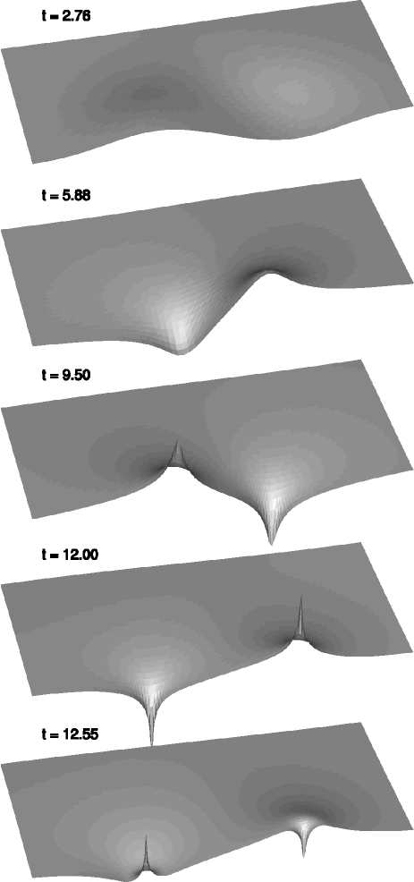
Figure 1: Several frames of $\Phi(\rho,z,t)$ from the evolution of near-critical, anti-symmetric initial data (10). The figures span the first several half-echoes of the local self-similar solutions, and the particular times shown correspond to when the scalar field reaches a local minima/maxima. The height of each surface represents the magnitude of $\Phi$, and the coordinate domain of each figure is $[0..2.5,-2.5..2.5]$ in $[\rho,z]$ (the axis $\rho=0$ is the nearest edge of each plot, and positive to negative $z$ runs from left to right).

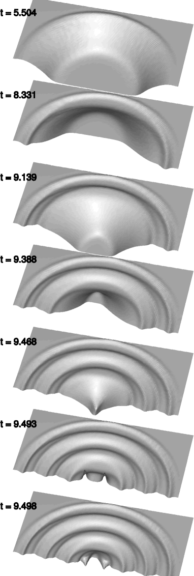
Figure 2: Several frames of $\Phi(\bar{r},\theta,t)$ from the evolution of near-critical, $\epsilon^{2}=3/4$ prolate initial data (9). Here we have transformed to coordinates $\bar{r}=\ln(\sqrt{\rho^{2}+z^{2}}+e_{0})-\ln e_{0}$ (with $e_{0}=2$x$10^{-4}$) and $\tan\theta=\rho/z$, to give a better view of the initial self-similar nature of the solution. $[\bar{r},\theta]$ ranges from $[0..\approx 10.8,0..\pi]$, with the axis $\rho=0$ being the nearest edge in each figure. The height of each surface represents the magnitude of $\Phi$. The times shown correspond to the times when $\Phi$ reaches a local minima/maxima, demonstrating the bifurcation that occurs after about $2$ self-similar echoes of the field.

With double precision arithmetic, we are able to tune the initial amplitude of a given family to within a part in $10^{15}$ of threshold, corresponding to about 3 full echoes of the spherically symmetric critical solution. The growth of the instability is sufficiently small that after 3 echoes we do not yet see a bifurcation for $\epsilon^{2}\leq 2/3$; for $\epsilon^{2}=3/4$ and $\epsilon^{2}=5/6$ we see a bifurcation after approximately $2$ and $1$ $1/2$ echoes respectively.

$\epsilon^{2}$	$\gamma$	$\langle\Delta\rangle^{1}$	$\langle\Delta\rangle^{2}$	$\langle|\Phi_{c}|\rangle$
$0$	$0.382\pm 2\%$	$3.44\pm 1\%$	$3.49\pm 3\%$	$0.431\pm 2\%$
$1/3$	$0.380\pm 2\%$	$3.41\pm 1\%$	$3.43\pm 3\%$	$0.431\pm 2\%$
$1/2$	$0.375\pm 3\%$	$3.37\pm 1\%$	$3.39\pm 4\%$	$0.430\pm 2\%$
$2/3$	$0.346\pm 3\%$	$3.13\pm 1\%$	$3.08\pm 4\%$	$0.419\pm 3\%$
$3/4(a)$	$0.313\pm 4\%$	$2.87\pm 4\%$	$3.03\pm 5\%$	$0.396\pm 6\%$
$3/4(b)$	$0.40\pm 10\%$	—	$\approx 3$	$0.40\pm 8\%$
$5/6(a)$	$0.28\pm 10\%$	$\approx 2$	$\approx 1$	$0.36\pm 7\%$
$5/6(b)$	$0.41\pm 10\%$	—	$\approx 3$	$0.36\pm 10\%$
AS	$0.383\pm 2\%$	—	$3.49\pm 3\%$	$0.434\pm 3\%$

Table 1: Critical parameters of the prolate families (9) and the anti-symmetric family ($AS$) (10). $\gamma$ is obtained from a least-squares fit to the data shown in Figure 4, $\langle\Delta\rangle^{1}$ is the average value of $\Delta$ measured between adjacent extremes in $\Phi_{c}$ as shown in Figure 5 (only using data from intermediate times), $\langle\Delta\rangle^{2}$ is the average value of $\Delta$ inferred from the periodic oscillations in Figure 4, and $\langle|\Phi_{c}|\rangle$ is the average absolute value of the extremes of $\Phi_{c}$ in Figure 5 (again using data from intermediate times). For the two prolate cases that bifurcate—$\epsilon^{2}=3/4$ and $\epsilon^{2}=5/6$—we list estimates of these parameters (where possible) before (a) and after (b) the bifurcation. For the anti-symmetric case, we do not have data for $\Phi_{c}$ versus central proper time; $\langle|\Phi_{c}|\rangle$ in that case is calculated as half the average difference between subsequent local extremes in $\Phi(\rho=0,z,t)$ about one of the local self-similar solutions. See the text for a discussion on how the estimated uncertainties were calculated.

Table 1 summarizes measurements made of the critical parameters—namely $\gamma,\Delta$ and the amplitude of each echo in $\Phi$—from the $\tau_{m0}/4$ simulations for each family of initial data (except for the $\epsilon^{2}=5/6$ case, where the increasing computational demands, resulting from larger, more elongated grids that are produced in the hierarchy for higher values of $\epsilon$, prevented us from computing with anything but $\tau_{m}=\tau_{m0}$). For the two simulations with the largest values of $\epsilon$, we list parameters obtained before and after the bifurcation, where possible. As with the anti-symmetric case, our method of geodesic integration cannot track moving centers, and so we cannot provide a direct estimate of $\Delta$ after a bifurcation. Also, for the $\epsilon^{2}=5/6$ case, we do not see a very distinctive periodic oscillation in the $\ln R_{\rm m}$ vs. $\ln\bar{p}$ plot, and thus can only provide a rough guess for $\Delta$ from that information. Most of the data in this table was gathered from Figures 4 and 5, which show $\ln R_{\rm m}$ vs. $\ln\bar{p}$ (with the linear relationship from the spherical family subtracted to better differentiate the plots) and $\Phi_{c}$, the central value of $\Phi$, vs. logarithmic central proper time for the prolate families prior to bifurcation, respectively. Also, Figure 3 shows the same type data displayed in Figure 5, but for the case $\epsilon=0$, and with the addition of an overlay of data obtained with a spherically symmetric 1D code choptuik . The good agreement between the results from the axisymmetric and spherical computations provides a measure of confidence in the correctness and level of accuracy of our 2D code.

The quoted uncertainty of a given value in Table 1 was calculated as the sum of the estimated truncation error from a convergence calculation using the different $\tau_{m}$ runs, and the standard deviation from the relevant averaging/fitting operation (except for $\epsilon^{2}=5/6$, where we could not estimate the truncation error as we only have data from a single value of $\tau_{m}$). However, in a sense these uncertainties are “optimistic,” for we have not accounted for possible systematic errors. Chief among these (in particular away from spherical symmetry) are the assumptions of discrete self-similarity, which was used to define $\tau^{\star}$ in Fig.5, and the assumption that the linear and periodic parts of Fig.4 are directly related to $\gamma$ and $\Delta$ respectively. For several of the simulations we have checked that the following numerical parameters are not significant sources of systematic error: outer boundary location, Dirichlet vs. Neumann conditions on $\alpha,\beta^{\rho}$ and $\beta^{z}$ at the outer boundary, and free vs. constrained evolution for $\psi$.

Figure 3: Comparison between results from our 2D axisymmetric code ($\epsilon=0$ initial data) and a 1D spherically symmetric code choptuik . Plotted is the central value of $\Phi$ as a function of logarithmic central proper time, for the most nearly critical simulations obtained in either case.

Note that our coordinate system is not adapted to spherical symmetry, and during an evolution of $\epsilon=0$ initial data, spherical symmetry is only preserved to within an amount proportional to the truncation error, and so will eventually exhibit the apparent second growing mode. In a certain sense this is a desirable feature, for at late times during an $\epsilon=0$ evolution this mode is the only one (apart from the unstable spherical mode) that should be visible perturbing the spherical solution; an $\epsilon>0$ evolution exhibits a host of additional, decaying asymmetric modes that prevent us from easily measuring the properties of the non-spherical growing mode. To this end, in Figure 6 we show plots of the maximum absolute value of the $\ell=2$ ($m=0$) spherical harmonic component of $\Phi$, denoted $\Phi_{\ell 2}$, in near-critical $\epsilon=0$ collapse, as measured along outgoing null slices of the spacetime (in other words, we decompose $\Phi(x,\theta_{0})$, constructed as described in Sec. II, into its spectral coefficients for each $x$—the $\ell=2$ component is $\Phi_{\ell 2}$.). We show results from simulations with 3 different values of the maximum truncation error estimate $\tau_{m}$, demonstrating the expected behavior that $\Phi_{\ell 2}\rightarrow 0$ in the limit $\tau_{m}\rightarrow 0$.

  

Figure 4: Plots of the logarithm of the maximum absolute value $|R_{\rm m}|$ attained by the Ricci scalar, during sub-critical evolution, vs. the logarithm of the distance in parameter space $\bar{p}=p^{\star}-p$ from the (estimated) critical parameter $p^{\star}$, for all families of initial data considered (using the lowest $\tau_{m}$ data). To avoid clutter in the figure, we have placed the data from each family on one of two identical panels. To facilitate comparison, the line $-2\gamma_{0}\ln\bar{p}$ has been subtracted from each curve, with $\gamma_{0}=0.382$ (the estimated value from the $\epsilon=0$ family). Also, the intercept of each curve has been set to $\bar{p}=0$. The estimated linear relationships used to calculate $\gamma$ in Table 1 are also shown in the figure.

Figure 5: The central value of $\Phi$ as a function of logarithmic central proper time, from the most nearly critical simulations of the prolate collapse families. The horizontal axis for each family was shifted so that the first maximum of each curve occurs at $-\ln(\tau-\tau^{\star})=0$. $\tau^{\star}$ is the accumulation point of each family (prior to the bifurcation for the $\epsilon^{2}=3/4$ and $\epsilon^{2}=5/6$ cases), calculated by assuming that the intermediate time behavior is discretely self-similar, and then finding the $\tau^{\star}$ for each case that minimizes the variance in $\Delta$ computed between pairs of adjacent minima/maxima in $\Phi_{c}$. To aid in comparison, dashed vertical lines have been drawn at intervals of $3.44$ in $\tau$, which is the estimated spherical echoing exponent.

We now argue that Fig. 6 also gives some evidence that the instability we do see in the numerical solution may be an actual feature of the continuum solution, and not a truncation-error-driven phenomenon.

Assume that the numerical solution has a well-behaved Richardson expansion. Then we expect any well-defined continuum property of the solution, such as the growth rate, $\lambda_{i}$, of a perturbative mode to have a similar expansion:

$$\hat{\lambda}_{i}=\lambda_{i}+hf(\vec{x})+O(h^{2}),$$ (11)

where $\hat{\lambda}_{i}$ is the numerically measured growth rate, $h$ is the discretization scale (we have assumed a first order accurate discretization), and $f(\vec{x})$ is some function of the continuum solution variables $\vec{x}$. Of course, in an adaptive scheme there is no single scale $h$; however, individual grids within the hierarchy do admit Richardson expansions, and hence we can loosely think of (11) holding over the hierarchy with some effective $h$ that would be related to the maximum truncation error estimate $\tau_{m}$. In martin_garcia_gundlach , the real part of the largest eigenvalue of any non-spherical mode perturbing the critical solution was found to be $\lambda_{2}\approx-0.02$; i.e. a decaying mode, and the corresponding eigenfunction had the angular dependence of the $\ell=2,m=0$ spherical harmonic $Y^{\ell}_{m}$. This magnitude of decay is about 100 times smaller than the growth rate of the dominant spherically symmetric mode, that has $\lambda=1/\gamma\approx 2.7$. Thus, looking at (11), it is certainly plausible that in a numerical scheme, even if $h$ were small enough to reasonably accurately model the dominant feature of a solution (as we evidently are from the comparison in Figure 3), it might still be large enough to significantly affect sub-dominant features of the solution, such as a small $\lambda_{i}$ in (11).

We should then be able to see a significant effect when changing $h$; however, in Figure 6, even though the initial amplitude of the asymmetry decreases as $\tau_{m}$ decreases (as expected), the apparent growth rate that we obtain, namely $\lambda_{2}\approx 0.1-0.4$, does not noticeably change within the relatively large uncertainty of the measurement. On the other hand, we may still be too far from the convergent regime to measure $\lambda_{2}$ (so that higher order terms in (11) are still important). Note that we also cannot conclusively say that the growing mode we see has a pure $\ell=2$ angular dependence, but it appears that the $\ell=2$ mode is at least an order of magnitude larger than any of the other asymmetric modes we find in the spectral decomposition. However, it must be noted that for computations with any of the three values of $\tau_{m}$ adopted we use 50 points in $\theta$ along which we integrate null curves, and so do not have good accuracy for determining the higher $\ell$ modes.

In Figure 7 below we show a plot of the growth rate of $\Phi_{\ell 2}$ from $\epsilon^{2}=2/3$ near critical solutions. This value of $\epsilon$ is the smallest, non-zero value considered that clearly shows growth of the asymmetry during the roughly three self-similar echoes of evolution; in the $\epsilon^{2}=1/3$ and $\epsilon^{2}=1/2$ cases, early-time evolution of the $\ell=2$ spectral component is dominated by decaying modes. For the $\epsilon^{2}=2/3$ data in Figure 7 we apparently are converging to the growth shown; i.e. as was the case for the spherically symmetric initial data, the growth does not appear to be truncation error dominated. Estimates of the growth rate from the simulation with the smallest value of $\tau_{m}$ gives $\lambda_{2}\approx 0.05-0.15$. However, this is quite a rough estimate as we cannot disentangle the supposed growing mode from the full spectrum of $\ell=2$ modes contributing to the plot shown in Figure 7.

Although we appear to be converging to a growth of the asymmetry in the $\epsilon^{2}=2/3$ case, and to a bifurcation for the $\epsilon^{2}=3/4$ case, this does not necessarily prove that the spherically symmetric critical solution has a second unstable mode. These families are sufficiently aspherical that one can imagine that the bifurcation is due to some artifact of the initial data—in particular a “focusing” effect, as the wave front of an imploding, prolate distribution of the scalar field will tend to focus to two locations on the axis, above and below the origin. If this is the case though, it is rather surprising that we see self-similar collapse occur about a single center prior to the bifurcation.

Figure 6: The maximum absolute value of the $\ell=2$ ($m=0$) spherical harmonic component of $\Phi$, $\Phi_{\ell 2}$, in near-critical $\epsilon=0$ collapse, measured along outgoing null slices of the spacetime, from simulations with 3 different values of the maximum truncation error estimate $\tau_{m}$. The graph indicates similar growth rates independent of the effective resolution. In order to better show the similarity of the growth rates, the data for the higher truncation error thresholds have been shifted along the horizontal axis which labels logarithmic central proper time (about $-3.4$ for the $\tau_{0}/2$ case and $-5.1$ for the $\tau_{0}/4$ data). Thus, at similar un-shifted times, the graph indicates that the amplitude of $\Phi_{\ell 2}$ decreases with $\tau_{m}$, as expected.

Figure 7: The maximum absolute value of the $\ell=2$ ($m=0$) spherical harmonic component of $\Phi$, $\Phi_{\ell 2}$, in near-critical $\epsilon^{2}=2/3$ collapse, measured along outgoing null slices of the spacetime, from simulations with 3 different values of the maximum truncation error estimate $\tau_{m}$. The horizontal axis labels the logarithmic central proper time when the given outgoing null surface intersects the origin. Note the different vertical scales when comparing this plot to the similar one for $\epsilon=0$ in Figure 6 (and we have not shifted the data here).

Finally, in Figure 8, we show comparisons of the “radial” profile of the $\ell=2$ spherical harmonic component of $\Phi$, measured along an outgoing null geodesic at (approximately) the same time within a self-similar echo, for the $\epsilon^{2}=0,\epsilon^{2}=2/3$ and anti-symmetric near-critical solutions (with $\tau_{m}=\tau_{m0}/4$). In the plot, the overall amplitude and affine distance along each null curve is rescaled so that the maximum amplitude is one, and occurs at one in rescaled affine time $\bar{x}$. That the curves from these representative families do approximately agree provides additional evidence that we are seeing a unique, asymmetric unstable mode.

Figure 8: The normalized $\ell=2$ ($m=0$) spherical harmonic component of $\Phi$, measured along an outgoing null geodesic starting from similar times within a (chosen) self-similar oscillation of the $\epsilon^{2}=0,\epsilon^{2}=2/3$ and anti-symmetric near critical solutions (from $\tau_{m}=\tau_{m0}/4$ simulations). To facilitate comparison, we have rescaled the amplitude of each curve so that the maximum is 1, and rescaled the affine parameter (labeled $\bar{x}$) along the null curves so that the first maxima of each is at $\bar{x}=1$.

IV Conclusion

We have presented results from a first study of scalar field critical collapse in axisymmetry in the fully non-linear regime. We find that critical phenomena is observed at the threshold of gravitational collapse of several families of asymmetric initial data. The critical solution that unfolds at threshold can (locally) be described as the spherically symmetric critical solution found in choptuik , with asymmetric perturbations. However, in contrast to the results of martin_garcia_gundlach , we find some evidence that a single $\ell=2$ spherical harmonic perturbation does not decay with time; rather it grows at a rate of roughly $1/10$ the magnitude of the dominant, spherically symmetric unstable mode. The nature of this second unstable mode is such that it causes a self-similar threshold solution, with some asymmetry in it, to eventually bifurcate into two local, self similar solutions that again resemble the spherical threshold spacetime. If this second instability is indeed a property of the spherically symmetric critical solution, then presumably one (or both if the initial data has reflection symmetry) of the new self-similar solutions would bifurcate again, and so on, resulting in an infinite, “random walk” of bifurcations on ever decreasing scales. Thus the second instability would not completely destroy the universal nature of generic (axisymmetric) critical collapse, but rather would alter it in an intriguing, family dependent manner.

To conclusively answer 1) whether there is a second unstable mode, and if so 2) how the bifurcation ultimately affects the threshold solution, is beyond the capabilities of our current code. First, we are using double precision arithmetic, and this prohibits us from tuning closer than $1$ part in $10^{15}$ of the threshold. Because the echoing exponent of the spherically symmetric solution is (relatively speaking) so large, $1$ part in $10^{15}$ can only give us about three, complete self-similar echoes. This is far from ideal when trying to estimate the growth (or decay) rate of a mode that may have an e-folding time on the order of 10-20 echoes. Second, we would like to achieve higher accuracy than we have been able to attain so far. To do this with the current code will require that we parallelize it because we have already reached the practical limits (in terms of memory usage and runtime) imposed by the hardware to which we have access. Alternatively, one could write a code adapted to the spherical critical solution (for instance using spherical polar coordinates with a logarithmic radial coordinate). This would allow one to obtain greater resolution, with a given amount of resources, than what we can achieve with our more general purpose cylindrical coordinates. Of course, spherical polar coordinates would not be well suited to following a solution beyond a bifurcation, but it should be adequate to study the growth or decay of perturbations.

References

- (1) M.W. Choptuik, “Universality And Scaling in Gravitational Collapse Of a Massless Scalar Field”, Phys. Rev. Lett. 70, 9 (1993)
- (2) C. Gundlach, “Critical phenomena in gravitational collapse”, Phys. Rept., 376, 339 (2003); C. Gundlach, “Critical phenomena in gravitational collapse”, Living Rev.Rel. 2 1999-4, gr-qc/0001046
- (3) A. Wang, “Critical Phenomena in Gravitational Collapse: The Studies So Far”, Braz.J.Phys. 31, 188 (2001)
- (4) A.M. Abrahams and C.R. Evans, “Critical Behavior and Scaling in Vacuum Axisymmetric Gravitational Collapse”, Phys. Rev. Lett. 70, 2980 (1993); A.M. Abrahams and C.R. Evans, “Universality in Axisymmetric Vacuum Collapse”, Phys. Rev. D49, 3998 (1994);
- (5) S.L. Liebling, “Singularity Threshold of the Nonlinear Sigma Model Using 3D Adaptive Mesh Refinement”, Phys. Rev. D66, 041703(R) (2002)
- (6) T. Koike, T. Hara, and S. Adachi, “Critical Behavior in Gravitational Collapse of Radiation Fluid: A Renormalization Group (Linear Perturbation) Analysis”, Phys. Rev. Lett. 74, 5170 (1995); “Observation of Critical Phenomena and Self-similarity in the Gravitational Collapse of Radiation Fluid”, Phys. Rev. Lett. 72, 1782 (1994); P.C. Argyres, in Contributions from the G1 Working Group at the APS Summer Study on Particle and Nuclear Astrophysics and Cosmology in the Next Millennium, Snowmass, Colorado, June 29 - July 14 (1994), astro-ph/9412046
- (7) J. M. Martín-García and C. Gundlach, “All Nonspherical Perturbations of the Choptuik Space-Time Decay”, Phys.Rev. D59, 064031 (1999)
- (8) C. Gundlach, “Nonspherical Perturbations of Critical Collapse and Cosmic Censorship” Phys.Rev. D57, 7075 (1998); C. Gundlach, “Critical Gravitational Collapse of a Perfect Fluid: Nonspherical Perturbations”, Phys. Rev. D65, 084021 (2002)
- (9) M.W. Choptuik, E.W. Hirschmann, S.L. Liebling and F. Pretorius, “An Axisymmetric Gravitational Collapse Code”, Class.Quant.Grav 20, 1857 (2003), gr-qc/0301006
- (10) S.W. Hawking and G.F.R. Ellis, The Large Scale Structure of Space-Time, Cambridge, Cambridge University Press 1973
- (11) K.Maeda, M.Sasaki, T.Nakamura and S.Miyama, “A New Formalism of the Einstein Equations for Relativistic Rotating Systems”, Prog. Theor. Phys. 63, 719 (1980)
- (12) F. Pretorius, “Adaptive Mesh Refinement for Coupled Elliptic-Hyperbolic Systems”, in preparation.
- (13) D. Garfinkle and C. Gundlach, “Symmetry Seeking Space-Time Coordinates”, Class. Quant. Grav. 16, 4111 (1999).
- (14) D. Garfinkle and G.C. Duncan, “Scaling of Curvature in Sub-critical Gravitational Collapse”, Phys.Rev. D58, 064024 (1998)
- (15) M. Berger and J. Oliger, “Adaptive Mesh Refinement for Hyperbolic Partial Differential Equations”, J. Comp. Phys. 53, 484 (1984).