Limiting noises in gravitational wave detectors: guidance from their statistical properties.

Abstract

It is expected that interferometric gravitational wave detectors such as LIGO [(1)] will be eventually limited by fundamental noise sources like shot noise and Brownian motion, as well as by seismic noise. In the commissioning process, other technical noise sources (electronics noise, alignment fluctuations) limit the sensitivity and are eliminated one by one. We propose here a way to correlate the noise in the output of the gravitational wave detector with other detector and environmental signals not through their linear transfer functions (often unknown), but through their statistical properties. This could prove useful for identifying the frequency bands dominated by different noise sources in the final configuration, and also to help the commissioning process.

1 INTRODUCTION

It is expected that interferometric gravitational wave detectors such as LIGO will be eventually limited by fundamental noise sources like shot noise and Brownian motion, as well as by seismic noise. In the commissioning process, other technical noise sources (electronics noise, alignment fluctuations) limit the sensitivity and are eliminated one by one. We propose here a way to correlate the noise in the output of the gravitational wave detector with other detector and environmental signals not through their linear transfer functions (often unknown), but through their statistical properties. This method was very useful in distinguishing the frequency band where Brownian motion was dominant, from other bands where seismic noise was dominant, in Ref.2. This method could then prove useful for identifying the frequency bands dominated by different noise sources in the final configuration of gravitational wave detectors, and also to help the commissioning process. we present in this article some preliminary results obtained with data from the LIGO first Science Run (August 23-September 9, 2002)S1 .

2 NOISE STATISTICS IN FREQUENCY DOMAIN

For some special classes of noise, statistical properties in the frequency domain are well defined in standard textbooks BendatPiersol86 . Assume we are given a time series $x(t)$ digitized with a sampling time $\Delta t=1/f_{s}$, and measured over a time interval $T$: $x_{n}=x(t_{n})$, $t_{n}={0,\Delta t,...N\Delta t=T}$. We can then calculate an estimate of its power spectral density by averaging over K=N/M power spectral densities ${S_{x}}_{i}(f)$, i=1…K, calculated for shorter time intervals of duration $T/K$. If the process is random and stationary, each time series $x_{i}(t_{n})$ with M points $n=(i-1)N/K+1...iN/K$ is a representative of an ensemble we can use to calculate means and variances at each frequency $f_{k}=2k/f_{s}$.

$${S_{x}}_{i}(f_{k})=\frac{2\Delta t}{M}\left(\sum_{n,m=(i-1)M+1}^{iM}x_{n}x_{m}e^{-2i\pi(k-1)(n-m)/M}\right)$$

$$S_{x}(f_{k})=(1/K)\sum_{i=1}^{K}{{S_{x}}_{i}(f_{k})}.$$

We can also also calculate the standard deviation of each frequency bin:

$$E_{x}(f_{k})=(1/N)\sum\left({S_{x}}_{i}(f_{k})-S_{x}(f_{k})\right)^{2}$$

If the signal $x(t)$ is a stationary, Gaussian process, then the ratio $R(f)=E(f)/S(f)$ has a mean of one with a variance equal to $1/\sqrt{N}$. If the signal is a sine wave, then $E(f)$ will tend to zero. If the signal is a random, stationary background with impulsive transients (“glitches”) added, $E(f)$ will in general will be larger than one.

The output signal in gravitational wave detectors, as in many other complex experiments, is a sum of many different noise components. The statistical properties of the time series $x(t)$ , will strongly depend on the spectral shape of the signal. Detection of signals in the noise are most often done in the frequency domain for this reason; if they are done in the time domain, it is usually after applying filters to select signals in a frequency band of interest, and also whitening the data.

A very important problem, different than signal detection, is identifying the contributions of different noise sources to the final output signal. This is done while “commissioning” instruments such as gravitational wave detectors, and is the first step to help eliminate unwanted or unexpected sources of noise, dominant over the expected ultimate limiting sources of noise. In general, the diagnostics is done by assuming known linear processes from sources whose spectral density can be measured independently (electronics noise and seismic noise, for example). Then, a comparison is made in the frequency domain, of the expected noise (source noise through a linear transformation), with the measured output spectral density. In general, different noise sources will be dominant in different frequency bands. This method is efficient only when the transfer functions are well known. However, many times the transfer function is unknown, and difficult or impossible to measure.

The statistical properties of the signals of the dominant sources of noise should be preserved by linear transformations, and thus the features of the function $R(f)=E(f)/S(f)$ (i.e., whether it is larger than one, close to one, or smaller than one) provide an opportunity to recognize the sources of noise even without the knowledge of the transfer function. We provide some examples of possible uses for the noise diagnostics in signals from the LIGO gravitational wave detectors.

3 Noise in Gravitational Wave Detectors

In LIGO gravitational wave detectors, the signal which is later calibrated and interpreted as the gravitational wave signal is the error signal in a feedback loop, controlling a demodulated signal of a photocurrent detected at the antisymmetric port of the interferometer.

We present in Fig. 1 the power spectral density of this signal, taken during 1216 seconds of the continuous operation in the first Science Run of the LIGO Science Collaboration. We have used a sampling frequency of $f_{s}=$ 4096 Hz, took K=76 measurements of power spectra, each for a segment 16 seconds long. The frequency bins are 62.5 mHz wide.

We show in Fig. 1 the calculation of the function $R(f)=E(f)/S(f)$. For random, stationary noise we expect this function to be close to one, within $1/\sqrt{N}$, where $N$ is the number of averages. We show these error bars for this particular measurement, taken with N=16 averages of $E(f)$ and $S(f)$ calculated for 16 seconds intervals (for a total time of 1200 seconds). A large fraction of the points have the statistical character of random, stationary noise: 94% of the frequency bins have $R(f)$ within 23% (or $2/\sqrt{K}$ of the expected value of one. However, many other frequency bins have a value of $R(f)$ significantly larger or smaller than one. Indicated in Fig1 are the points with $R(f)$ outside a 3-$\sigma$ interval from unity. The largest values of $R$ are mostly concentrated in two frequency bands: 70-76 Hz and 280-300 Hz, corresponding to two small broad peaks in the amplitude spectral density. The frequencies with low values of $R$ (indicating possible periodic signals) are all narrow lines in the spectrum, mostly low harmonics of the 60 Hz AC line. Interestingly, high harmonics of the power line frequency ($\geq 420$ Hz) have high values of $R(f)$, opposed to the low harmonics ( $\leq 360$ Hz).

This simple calculation on a single signal shows already qualitative differences in the statistics of different frequency bands, showing that this strategy may prove very useful. Notice that the features of the function $R(f)$ are very different than the features in the amplitude spectral density. We now discuss in detail some further analysis of different frequency bands.

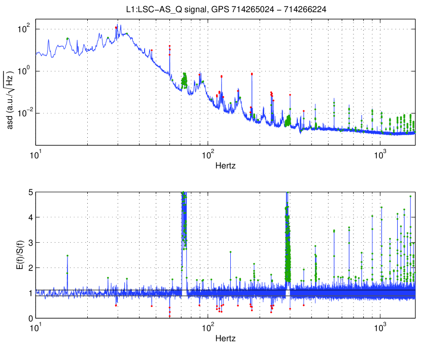
Figure 1: Top: Amplitude Spectral Density of the output of the LIGO Livingston Gravitational Wave Signal (the units of the raw signal are arbitrary). Bottom: The ratio of variance to mean in each frequency bin. The points indicate the bins outside a 2-$\sigma$ interval of a random, stationary noise source. The solid lines indicate 1-$\sigma$ deviation from unity.

3.1 Stationary frequency bands

Most of the frequency bins shown in Fig. 1 have statistics consistent with random, stationary noise. An example of the time history and histogram of the power in a single frequency bin is shown in Fig.2, for a frequency near 1kHz. We expect most ultimately limiting noise sources (Brownian motion,shot noise) and some of technical noise sources (electronic noise) to be random and stationary. This test, then, does not provide a particular mean to distinguish different noise sources if they are all random and stationary. As we see in the next examples, this is very often not the case.

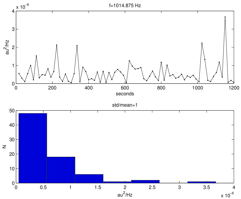
Figure 2: Top: time history of the power in the frequency bin indicated. Bottom: histogram of the values shown in top. The numerical ratio of variance to mean is 1+$7\times 10^{-8}$ (but of course the statistical error in the estimates of the mean and variance are larger, given by $1/\sqrt{K}=0.1$).

3.2 Two noisy frequency bands

As we noticed in Fig. 1, there are two broad frequency bands which are strongly non-stationary, [70-76] Hz and [280-300] Hz, corresponding to two small broad peaks in the amplitude spectral density. Notice that the frequency resolution in the analysis (63 mHz) allows us to distinguish the properties of the 300 Hz frequency bin, with R=0.37 (indicating periodicity), from its two neighboring bins, with R=0.9 (indicating random stationary noise), and from lower frequency bins: the bin at 299.9375 Hz has R=2.1, indicating strong non-stationary behavior.

If we plot the power in each frequency bin as a function of time, for each 16 seconds time segment used in the ensemble, we notice that usually the culprit for the non-stationary behavior is one or two points with a large excess power, or a “glitch”. These glitches happen, however, at different times in the different frequency bins, as shown in Fig. 3. Since the glitches are concentrated in definite frequency bands, it is likely that the source of non-stationarity in each band is common; however it it clear that the source produces recurrent glitches in slightly different frequency bins. This particular feature could be fruitfully used to recognize the characteristics in another signal, to help the identification of the noise source.

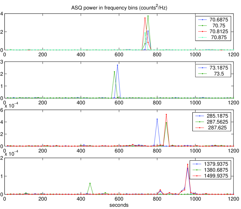
Figure 3: Time histories of power in different frequency bins that show a very non-stationary behavior, indicated by a ratio of variance to mean larger than 2.

3.3 Power lines: two different sources?

The harmonic frequencies of the AC power line, 60 Hz, are a special set. The low number harmonics have stationary, periodic structure rather than random, with a very low R, as shown in Fin.4: the power in the frequency bin has a mean significantly different from zero, and the histogram approximates a Gaussian away from zero rather than a Rayleigh distribution. This features disappears gradually for higher harmonics, where a non-stationary behavior is present, with the maximum power oscillating between neighboring frequency bins: this is typical of beating of lines, where some lines are from th AC power and some from driven circuits or machinery which may lag the driving frequency.

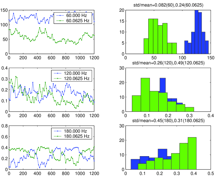
Figure 4: Time histories of power in frequency bins near harmonics of 60 Hz, and corresponding histograms.

4 Conclusions

We have shown that the study of statistical properties of signals in interferometric wave detectors is very useful to distinguish dominant sources of noise in different frequency bins. This may prove a powerful technique when analyzing progress and differences in the commissioning of interferometric gravitational wave detectors. It is already being used as a graphical monitor in the LIGO Science runs RayleighMon , as a qualitative measure of the data quality. We hope to use this method for more quantitative measures of the data quality, but more importantly, to find the sources of the non-stationary noise in the gravitational wave output.