High Speed Dynamics of Collapsing Cylindrical Dust Fluid

Abstract

We construct approximate solutions that will describe the last stage of cylindrically symmetric gravitational collapse of dust fluid. Just before the spacetime singularity formation, the speed of the dust fluid might be almost equal to the speed of light by gravitational acceleration. Therefore the analytic solution describing the dynamics of cylindrical null dust might be the crudest approximate solution of the last stage of the gravitational collapse. In this paper, we regard this null dust solution as a background and perform ‘high-speed approximation’ to know the gravitational collapse of ordinary timelike dust fluid; the ‘deviation of the timelike 4-velocity vector field from null’ is treated as a perturbation. In contrast with the null dust approximation, our approximation scheme can describe the generation of gravitational waves in the course of the cylindrically symmetric dust collapse.

I Introduction

The gravitational collapse and spacetime singularity formation are physically very significant phenomena predicted by general relativity. However since extremely high density, high pressure and large spacetime curvature will be realized around the spacetime singularity, all known theories of physics including general relativity could break down there and a quantum theory of gravity might be necessary to describe such physical situations. If this perspective is right, the appearance of the spacetime singularity predicted by general relativity has no rigorous meaning, since general relativity can not describe the gravitational processes in the neighborhood of the spacetime singularity. However, it is still important to study the spacetime structures around singularities by assuming general relativity, since such studies reveal what happens at the entrance of new physics, although there is an issue of their observability in connection with the cosmic censorshipRef:penrose69 .

A singularity visible for distant observers is called a globally naked singularity. Nakamura, Shibata and one of the present authors (NSN) have conjectured that the large spacetime curvature in the neighborhood of non-spherical spacetime singularities can propagate away to infinity in the form of gravitational radiation if those singularities are globally nakedRef:DRIES-UP . If this conjecture is true, formation processes of naked singularities are strong sources of gravitational radiation and thus might be one of the targets of gravitational wave astronomyRef:TAMA ; Ref:LIGO ; Ref:VIRGO ; Ref:GEO ; Ref:LISA . However, numerical simulations performed by Shapiro and Teukolsky suggested that the gravitational collapse of a collisionless gas spheroid might form a spindle naked singularity in accordance with the hoop conjectureRef:HOOP ; Ref:hoop-misc , but little gravitational radiation is generated in its formation processRef:Spindle . This seems to be a counter example against NSN’s conjecture. However it should be noted that the numerical accuracy of the simulations performed by Shapiro and Teukolsky seems to be insufficient to give a definite statementRef:DRIES-UP .

Motivated by the work of Shapiro and Teukolsky, Echeverria performed numerical simulations with very high resolution for the cylindrically symmetric gravitational collapse of an infinitely thin dust shellRef:Dust-Shell . Although infinitely long cylindrical matter or radiation is unrealistic, this system could be a crude approximation of sufficiently thin and long but finite length distribution like as the case of spindle gravitational collapse simulated by Shapiro and Teukolsky. As Thorne showed, the gravitational collapse of a cylindrical matter with a compact support in the radial direction does not form a black hole horizon (marginal surface)Ref:HOOP . Thus the singularities formed in the simulations by Echeverria must be globally naked. Further Echeverria’s numerical results showed that the gravitational collapse of the cylindrical dust shell causes gravitational wave burst. Thus in this case, the naked singularity formation is really a strong source of gravitational radiation. This seems to be inconsistent with Shapiro and Teukolsky.

By the same motivation as that of Echeverria, Chiba investigated the gravitational collapse of cylindrically distributed dust fluid, which also forms a naked singularity. Then Chiba’s numerical results imply that the gravitational radiation generated by dust collapse is extremely smallRef:Chiba . This is consistent with the results by Shapiro and Teukolsky and further with Piran’s numerical simulations for the gravitational collapse of cylindrical perfect fluid with the adiabatic index $4/3\leq\Gamma\leq 2$; softer equation of state leads to less emission of gravitational wavesRef:Piran .

In this paper, in order to clarify the reason of the apparent inconsistency between Echeverria’s work and the others, and further to understand the generation mechanism of gravitational radiation in the formation of linear singularities, we investigate the dynamics of the cylindrically symmetric dust fluid by the analytic procedure. Here we should note that it is rather dangerous to accept numerical results, especially these for structures around spacetime singularities, without any consistency checks. In this sense, it is also of great significance to obtain approximate solutions by completely or almost analytic procedures, which could complement the numerical studies.

A few exact solutions for cylindrical gravitational collapse are known. One is that describing the gravitational collapse of null dustRef:Morgan ; Ref:LW ; Ref:Nolan , which is a cylindrically symmetric version of Vaidya solutionRef:DJ89 . As gravitational collapse proceeds, the speed of collapsing matter might approach to the speed of light. Thus the null dust is often regarded as the crudest approximation of the last stage of gravitational collapse. However the cylindrical null dust does not generate gravitational radiation. Recently, Pereira and Wang constructed analytic model of the cylindrical thin shell made of counter rotating dust particlesRef:PW . This exact solution might be useful and physically significant, but unfortunately, it is impossible to describe the generation of gravitational radiation near the spacetime singularityRef:GJ . Here we would like to comment on Echeverria’s analytic work. Echeverria analytically constructed an asymptotic solution for the gravitational collapse of an infinitely thin dust shell by using the numerical results and further by putting self-similar ansatzRef:Dust-Shell . Although Echeverria’s asymptotic solution might describe the generation of gravitational waves, the behavior of the infinitely thin shell might be different from that of finitely distributed masses. Therefore in order to see the gravitational wave generation in more general situations analytically, we need new exact solutions or new approximation scheme.

In this paper, we perform a kind of perturbation analysis on the null dust solution by assuming that the speed of the collapsing dust is almost equal to the speed of light. We stress that the generation of gravitational radiation can be described by this approximation scheme.

This paper is organized as follows. In Sec.II, we present the basic equations of the cylindrically symmetric dust system. In Sec.III, we derive the equations and solutions of our approximation scheme to describe the gravitational collapse with almost the speed of light; we explicitly show solutions for thin and thick dust shells, separately. Finally, Sec.IV is devoted for summary and discussion of the physical meaning of our solutions by comparing those with the previous studies.

In this paper, we adopt $c=1$ unit.

II Cylindrically Symmetric Dust System

In this paper, we assume the whole-cylinder symmetry which leads to the following line elementRef:MelvinI ; Ref:C-energy ; Ref:MelvinII ,

$$ds^{2}=e^{2(\gamma-\psi)}\left(-dt^{2}+dr^{2}\right)+e^{2\psi}dz^{2}+e^{-2\psi}R^{2}d\varphi^{2},$$ (1)

where $\gamma$, $\psi$ and $R$ are functions of $t$ and $r$. Then Einstein equations are

$$\gamma^{\prime}=\left({R^{\prime}}^{2}-{\dot{R}}^{2}\right)^{-1}\biggl{\{}RR^{\prime}\left({\dot{\psi}}^{2}+{\psi^{\prime}}^{2}\right)-2R{\dot{R}}{\dot{\psi}}\psi^{\prime}+R^{\prime}R^{\prime\prime}-{\dot{R}}{\dot{R}}^{\prime}$$

$$~{}~{}~{}~{}-8\pi G\sqrt{-g}\left(R^{\prime}T^{t}{}_{t}+{\dot{R}}T^{r}{}_{t}\right)\biggr{\}},$$ (2)

$${\dot{\gamma}}=-\left({R^{\prime}}^{2}-{\dot{R}}^{2}\right)^{-1}\biggl{\{}R{\dot{R}}\left({\dot{\psi}}^{2}+{\psi^{\prime}}^{2}\right)-2RR^{\prime}{\dot{\psi}}\psi^{\prime}+{\dot{R}}R^{\prime\prime}-R^{\prime}{\dot{R}}^{\prime}$$

$$~{}~{}~{}~{}-8\pi G\sqrt{-g}\left({\dot{R}}T^{t}{}_{t}+R^{\prime}T^{r}{}_{t}\right)\biggr{\}},$$ (3)

$${\ddot{\gamma}}-\gamma^{\prime\prime}={\psi^{\prime}}^{2}-{\dot{\psi}}^{2}-{8\pi G\over R}\sqrt{-g}T^{\varphi}{}_{\varphi},$$ (4)

$${\ddot{R}}-R^{\prime\prime}=-8\pi G\sqrt{-g}\left(T^{t}{}_{t}+T^{r}{}_{r}\right),$$ (5)

$${\ddot{\psi}}+{{\dot{R}}\over R}{\dot{\psi}}-\psi^{\prime\prime}-{R^{\prime}\over R}\psi^{\prime}=-{4\pi G\over R}\sqrt{-g}\left(T^{t}{}_{t}+T^{r}{}_{r}-T^{z}{}_{z}+T^{\varphi}{}_{\varphi}\right),$$ (6)

where $g$ is the determinant of the metric tensor, a dot means the derivative with respect to $t$ while a prime means the derivative with respect to $r$.

In this paper, we consider dust fluid. The stress-energy tensor is

$$T^{\mu\nu}=\rho u^{\mu}u^{\nu},$$ (7)

where $\rho$ is the rest mass density and $u^{\mu}$ is the 4-velocity field; all these matter variables depend on $t$ and $r$ only. By the assumption of the whole-cylinder symmetry, the components of the 4-velocity $u^{\mu}$ are written as

$$u^{\mu}=u^{t}\left(1,-1+V,~{}0,~{}0\right).$$ (8)

By the normalization $u^{\mu}u_{\mu}=-1$, $u^{t}$ is expressed as

$$u^{t}={e^{-\gamma+\psi}\over\sqrt{V\left(2-V\right)}}.$$ (9)

Here we introduce a new density variable $D$ defined by

$$D:={\sqrt{-g}\rho u^{t}\over\sqrt{V\left(2-V\right)}}={Re^{\gamma-\psi}\rho\over V\left(2-V\right)}.$$ (10)

The components of the stress-energy tensor are then expressed as

$$\sqrt{-g}T^{t}{}_{t} = -e^{\gamma-\psi}D,$$ (11)

$$\sqrt{-g}T^{r}{}_{t} = e^{\gamma-\psi}D(1-V)=-\sqrt{-g}T^{t}{}_{r},$$ (12)

$$\sqrt{-g}T^{r}{}_{r} = e^{\gamma-\psi}D(1-V)^{2},$$ (13)

and the other components vanish. The equation of motion $\nabla_{\beta}T^{\beta}{}_{\alpha}=0$ ($\nabla_{\beta}$ is the covariant derivative) leads to

$$\partial_{u}D = -{1\over 2}(DV)^{\prime}+{D\over 2}(1-V)\left\{2\partial_{u}\left(\psi-\gamma\right)-V\left({\dot{\psi}}-{\dot{\gamma}}\right)\right\},$$ (14)

$$D\partial_{u}V = (1-V)\partial_{u}D+{1\over 2}\left\{V\left(1-V\right)D\right\}-{D\over 2}\left\{2\partial_{u}\left(\psi-\gamma\right)-V({\dot{\psi}}-{\dot{\gamma}})\right\},$$ (15)

where $u=t-r$ is the retarded time and $\partial_{u}$ is the partial derivative of $u$ with the advanced time $v=t+r$ fixed.

To estimate the energy released in the form of gravitational radiation, the $C$-energy and its flux vector proposed by ThorneRef:C-energy is useful. The $C$-energy $E$ is given as

$$E:={1\over 8}\left\{1-e^{-2\psi}\left(\nabla^{\alpha}R\right)\left(\nabla_{\alpha}R\right)\right\}.$$ (16)

Then the flux vector $J^{\mu}$ associated with $E$ is introduced as

$$\sqrt{-g}J^{\mu}={1\over 2\pi}(\partial_{r}E,~{}\partial_{t}E,~{}0,~{}0).$$ (17)

As shown by Hayward, if the null energy condition is satisfied, $\zeta^{\alpha}\nabla_{\alpha}E\geq 0$ for any achronal vector $\zeta^{\alpha}$, and hence $0\leq E<1/8$ holds outside the causal future of the naked singularityRef:Hayward . Note that the conservation law $\nabla_{\mu}J^{\mu}=0$ is trivially satisfied. Using Einstein equations, the energy flux vector $J^{\mu}$ is expressed as

$$\sqrt{-g}J^{t} = {e^{-2\gamma}\over 8\pi G}\biggl{\{}RR^{\prime}({\dot{\psi}}^{2}+{\psi^{\prime}}^{2})-2R{\dot{R}}{\dot{\psi}}\psi^{\prime}-8\pi G\sqrt{-g}(R^{\prime}T^{t}{}_{t}+{\dot{R}}T^{r}{}_{t})\biggr{\}},$$ (18)

$$\sqrt{-g}J^{r} = {e^{-2\gamma}\over 8\pi G}\biggl{\{}R{\dot{R}}({\dot{\psi}}^{2}+{\psi^{\prime}}^{2})-2RR^{\prime}{\dot{\psi}}\psi^{\prime}-8\pi G\sqrt{-g}(R^{\prime}T^{r}{}_{t}-{\dot{R}}T^{r}{}_{r})\biggr{\}},$$ (19)

and the other components vanish.

III The Gravitational Collapse of High Speed Dust

Echeverria showed that the speed of a collapsing cylindrical dust shell becomes faster and faster and finally almost equal to the speed of light. This seems to be a generic behavior near the spacetime singularity even in more general situations, and thus hereafter we focus on the situation in which speeds of dust fluid elements are almost equal to the speed of light. On the ground of physics, such a situation can be well approximated by Morgan’s null dust solutionRef:Morgan . Then we treat the ‘deviation of the 4-velocity of the dust fluid from null’ as a perturbation and will perform a linear perturbation analysis.

First, we consider the null dust limit of the timelike dust fluid. The stress-energy tensor is rewritten as

$$T_{\mu\nu}={e^{-3(\gamma-\psi)}D\over R}k_{\mu}k_{\nu},$$ (20)

where

$$k^{\mu}=(1,-1+V,~{}0,~{}0).$$ (21)

In the limit of $V\rightarrow 0$, $k^{\mu}$ approaches to the null vector and hence $T_{\mu\nu}$ agrees with that of null dust if this limit is taken with $D$ fixed. Here note that the limit of $V\rightarrow 0$ with $D$ fixed leads to vanishing rest mass density $\rho\rightarrow 0$, i.e., massless field (see Eq.(10)). Thus for $0<V\ll 1$, in order to obtain the approximate solutions for the metric variables, the stress-energy tensor could be replaced by that of collapsing null dust.

Assuming that $\psi$ vanishes initially, the solutions of the complete null dust are easily obtained as

$$\psi = 0,$$ (22)

$$\gamma = \gamma_{B}(v),$$ (23)

$$R = r,$$ (24)

$$8\pi GDe^{\gamma_{B}} = {d\gamma_{B}\over dv},$$ (25)

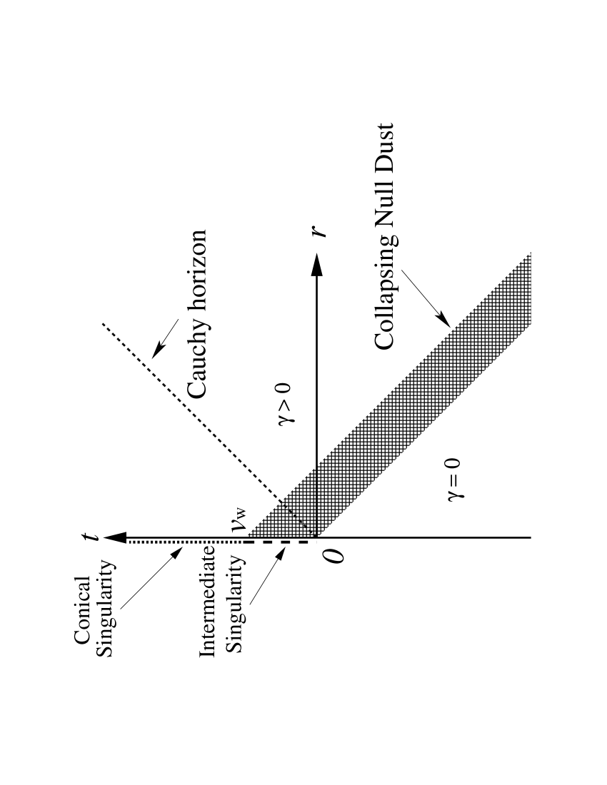
Figure 1: Morgan’s cylindrical null dust solution. There is the null dust in the shaded region; $D(v)>0$ for $0<v<v_{\rm w}$. The dashed line on $t$-axis corresponds to the intermediate singularity at which an observer suffers infinite tidal force although any scalar polynomials of the Riemann tensor do not vanish. On the other hand, the dotted line on $t$-axis is the conical singularity. The Cauchy horizon is short dashed line of $t=r$.

where $\gamma_{B}(v)$ is an arbitrary function of the advanced time $v$Ref:Morgan . This solution was studied by Letelier and WangRef:LW and Nolan in detailRef:Nolan . If the density variable $D$ does not vanish at $r=0$, there is the naked singularity; this is not a scalar polynomial singularity but intermediate one at which observers suffer infinite tidal force although all the scalar polynomials of the Riemann tensor do not divergeRef:LW . The situation is depicted in Fig.1. In this figure, we assume that the density variable $D$ has a compact support with respect to the advanced time $v$, i.e., $D>0$ for $0<v<v_{\rm w}$. As mentioned, we will regard this solution as a background spacetime.

We introduce a small parameter $\epsilon$ and assume the order of the variables as $V=O(\epsilon)$ and $\psi=O(\epsilon)$. Further we rewrite the variables $\gamma$, $R$ and $D$ as

$$e^{\gamma} = e^{\gamma_{B}}(1+\delta_{\gamma}),$$ (26)

$$R = r(1+\delta_{R}),$$ (27)

$$D = D_{B}(1+\delta_{D}),$$ (28)

and assume that $\delta_{\gamma}$, $\delta_{R}$ and $\delta_{D}$ are also $O(\epsilon)$, where

$$D_{B}(v):={1\over 8\pi Ge^{\gamma_{B}}}{d\gamma_{B}\over dv}.$$ (29)

We would like to call the perturbative analysis with respect to this small parameter $\epsilon$ ‘the high-speed approximation’.

The 1st order equations with respect to $\epsilon$ are given as follows; the Einstein equations lead to

$$\delta_{\gamma}{}^{\prime}=8\pi Ge^{\gamma_{B}}D_{B}\left\{\delta_{\gamma}-\psi+\delta_{D}-2\partial_{v}(r\delta_{R})\right\}+(r\delta_{R})^{\prime\prime},$$ (30)

$${\dot{\delta}}_{\gamma}=8\pi Ge^{\gamma_{B}}D_{B}\left\{\delta_{\gamma}-\psi+\delta_{D}-2\partial_{v}(r\delta_{R})-V\right\}+(r{\dot{\delta}_{R}})^{\prime},$$ (31)

$${\ddot{\delta}}_{\gamma}-\delta_{\gamma}{}^{\prime\prime}=0,$$ (32)

$$r{\ddot{\delta}}_{R}-(r\delta_{R})^{\prime\prime}=16\pi Ge^{\gamma_{B}}D_{B}V,$$ (33)

$${\ddot{\psi}}-\psi^{\prime\prime}-{1\over r}\psi^{\prime}={8\pi G\over r}e^{\gamma_{B}}D_{B}V,$$ (34)

where $\partial_{v}$ is the partial derivative of the advanced time $v$ with fixed retarded time $u$; the conservation law (14) leads to

$$\partial_{u}\left(\delta_{D}+\delta_{\gamma}-\psi\right)=-{e^{\gamma_{B}}\over 2D_{B}}\left\{V{d\over dv}\left(e^{-\gamma_{B}}D_{B}\right)+V^{\prime}e^{-\gamma_{B}}D_{B}\right\};$$ (35)

the Euler equation (15) reads as

$$\partial_{u}V=0,$$ (36)

where we have used Eq.(14). Equation(36) means that $V$ is an arbitrary function of the advanced time $v$, i.e.,

$$V=V(v).$$ (37)

This implies that $V$ does not vanish even in the limit to the spacetime singularity.

Since we solve the basic equations (30)-(36) as a Cauchy problem, we have to set initial data for these equations. Our purpose is to study the generation mechanism of gravitational radiation in the formation process of the naked singularity. Therefore we set almost all the perturbation variables to vanish at some moment before the formation of the naked singularity. More concretely speaking, we set the initial data as

$$\delta_{\gamma}=\delta_{R}={\dot{\delta}}_{R}=\psi={\dot{\psi}}=\delta_{D}=0~{}~{}~{}~{}~{}~{}{\rm at}~{}~{}t=t_{\rm i},$$ (38)

where $t_{\rm i}$ is chosen so that the spacetime singularity of the background does not form before and at $t=t_{\rm i}$. Then we may recognize the formation process of the singularity as an origin of the perturbation variables generated after $t=t_{\rm i}$. Here note that these initial conditions are consistent with Eq.(30).

It should be noted that $V$ and ${\dot{\delta}}_{\gamma}$ have to have non-trivial values at $t=t_{\rm i}$. Since we consider the timelike dust, $V$ must not vanish. Due to this constraint and Eq.(31), ${\dot{\delta}}_{\gamma}$ has non-trivial value at $t=t_{\rm i}$ as

$${\dot{\delta}}_{\gamma}(t_{\rm i},r)=-S(t_{\rm i}+r),$$ (39)

where for notational simplicity, we have introduced a new variable $S$ defined by

$$S(v):=8\pi Ge^{\gamma_{B}}D_{B}V.$$ (40)

For $t\geq t_{\rm i}$, the solution of $\delta_{\gamma}$ satisfying the initial conditions (38) and (39) is obtained as

$$\delta_{\gamma}(t,r;t_{\rm i})={1\over 2}\left\{\Theta(t_{\rm i}-u)\int_{t_{\rm i}-u}^{v-t_{\rm i}}+\Theta(u-t_{\rm i})\int_{u-t_{\rm i}}^{v-t_{\rm i}}\right\}dxS(t_{\rm i}+x),$$ (41)

where $\Theta(x)$ is Heaviside’s step function, and we have imposed a boundary condition $\delta_{\gamma}{}^{\prime}|_{r=0}=0$ so that the analyticity, or equivalently, the locally Minkowskian nature at the origin $r=0$ is guaranteed before the formation of the spacetime singularity there. We can also obtain a solution of Eq.(33) by the ordinary procedure to obtain the solutions of the wave equation in 2-dimensional Minkowski spacetime. Here we should note that $r\delta_{R}$ has to vanish at $r=0$ before the singularity formation. The solution satisfying this boundary condition is given as

$$\delta_{R}(t,r;t_{\rm i})={2\over\pi r}\int_{t_{\rm i}}^{t}d\tau\int_{0}^{\infty}dxS(\tau+x)\int_{0}^{\infty}{dk\over k}\sin(kr)\sin(kx)\sin\left\{k(t-\tau)\right\}.$$ (42)

We would like to express the solution of Eq.(34) in the form

$$\psi(t,r;t_{\rm i})=\int_{-\infty}^{+\infty}dv_{\rm s}S(v_{\rm s})\Psi(t,r;t_{\rm i},v_{\rm s}),$$ (43)

where by introducing the following function,

$$\Omega(t,r;x,y):={(t-y)^{2}-r^{2}-2(t-y)(x-y)\over 2r(x-y)},$$ (44)

$\Psi$ is expressed as

$$\Psi(t,r;t_{\rm i},v_{\rm s})={1\over\pi}\sqrt{2|t_{\rm i}-v_{\rm s}|\over r}\int_{\Omega(t,r;t_{\rm i},v_{\rm s})}^{1}{dz\over z+(t-v_{\rm s})/r}\sqrt{z-\Omega(t,r;t_{\rm i},v_{\rm s})\over 1-z^{2}}.$$ (45)

The detailed derivation of the above equation is given in Appendix. Eq.(35) can be easily integrated and the solution satisfying the initial condition (38) is obtained as

$$\delta_{D}=\psi-\delta_{\gamma}+(t_{\rm i}-t)\left(V{d\ln S\over dv}-2S\right).$$ (46)

The lowest order of the energy flux vector in the vacuum region is given by

$$\sqrt{-g}J^{t} = {r\over 8\pi G}\left({\dot{\psi}}^{2}+{\psi^{\prime}}^{2}\right),$$ (47)

$$\sqrt{-g}J^{r} = -{r\over 4\pi G}{\dot{\psi}}\psi^{\prime}.$$ (48)

Hence we need to know the solution for $\psi$ to see the energy flux at the future null infinity.

As mentioned, the symmetric axis $r=0$ with non-vanishing $D_{B}$ is the naked singularity of the background Morgan spacetime and will also be the naked singularity of the spacetime considered here. If $S(v)$ and $Vd\ln S/dv$ are functions defined in $r\geq 0$, the solutions of perturbation quantities (41)-(46) could be finitely defined in $t\geq t_{\rm i}$ and thus in the causal future of the naked singularity. This means that we could study the structure of the naked singularity defined by Eqs.(41)-(46). However here note that in general, in order to solve the causal future of naked singularities as a Cauchy problem, we need to impose some boundary conditions at the naked singularities. In reality, we have imposed the boundary conditions for the perturbation equations (32)-(34) at the naked singularity to obtain the solutions in the causal future of the naked singularity; the symmetric axis $r=0$ is locally Minkowskian.

By imposing this boundary condition, we constructed the Green’s function of each perturbation equation and then wrote down the solutions (41)-(43). However, after the formation of the background naked singularity, it is meaningless to impose the locally Minkowskian nature of the axis $r=0$, since the axis is singular. Hence we have to be careful to discuss the above solutions in the causal future of the naked singularity. For this reason, in this paper, we focus on the causal past of the Cauchy horizon only.

III.1 Thin Shell

First, we consider a thin shell, that is,

$$S=S_{\rm c}\delta(v),$$ (49)

where $S_{\rm c}$ is a positive constant and $\delta(v)$ is Dirac’s delta function. We set $V=V_{\rm c}=$constant. Since the spacetime singularity forms at $(t,r)=(0,0)$, we should choose the initial time $t_{\rm i}$ negative. The Cauchy horizon, which is the boundary of the causal future of the naked singularity, is given by $u=0$. From Eqs.(29) and (49), we obtain

$$\gamma_{B}={S_{\rm c}\over V_{\rm c}}\Theta(v),$$ (50)

where we have imposed the boundary condition, $\gamma_{B}=0$ at $r=0$, so that the symmetric axis $r=0$ is locally Minkowskian before the singularity formation.

In this thin shell case, as will be shown below, the high-speed approximation breaks down. This means that Echeverria’s numerical results for the gravitational collapse of a thin dust shell can not be recovered by our method. However, the solution of a thin shell is useful in constructing solutions for the thick shell case and hence we proceed to study this.

From Eq.(41), we obtain the solution for $\delta_{\gamma}$ as

$$\delta_{\gamma}(t,r;t_{\rm i})=-{S_{\rm c}\over 2}\left\{\Theta(2t_{\rm i}-u)-\Theta(v)\right\}.$$ (51)

From Eq.(42), we obtain the solution for $\delta_{R}$ in the region of $t\geq t_{\rm i}$ and of the causal past of the Cauchy horizon $u\leq 0$ as

$$\delta_{R}(t,r;t_{\rm i}) = {S_{\rm c}\over 2r}\bigl{[}\left(t-t_{\rm i}\right)\left\{\Theta(v)-\Theta(u)+\Theta(u-2t_{\rm i})-\Theta(v-2t_{i})\right\}$$ (52)

$$- {v\over 2}\Theta(u-2t_{\rm i})\Theta(v)+{u\over 2}\Theta(v-2t_{\rm i})\Theta(u)\bigr{]}.$$

Substituting Eq.(49) into Eq.(43), we obtain

$$\psi_{\rm s}(t,r;t_{\rm i})=S_{\rm c}\Psi(t,r;t_{\rm i},0).$$ (53)

In order to see the asymptotic behavior in approaching to the Cauchy horizon, we define a new variable $\varepsilon$ as

$$t=r(1-\varepsilon).$$ (54)

Then the function $\Psi$ is expressed as

$$\Psi(t,r;t_{\rm i},0)={1\over\pi}\sqrt{2|t_{\rm i}|\over r}\int_{0}^{2-\varepsilon_{2}}{\sqrt{x}dx\over(x+\varepsilon_{1})\sqrt{(x+\varepsilon_{2})(2-\varepsilon_{2}-x)}},$$ (55)

where we have introduced a new integration variable $x=z-\Omega(t,r;t_{\rm i},0)$ and

$$\varepsilon_{1} := {r\over|t_{\rm i}|}\varepsilon\left(1-{\varepsilon\over 2}\right),$$ (56)

$$\varepsilon_{2} := {r\over|t_{\rm i}|}\varepsilon\left(1+{|t_{\rm i}|\over r}-{\varepsilon\over 2}\right).$$ (57)

The limit of $\varepsilon\rightarrow 0_{+}$ with $r$ fixed corresponds to the limit to approach the Cauchy horizon from its chronological past. We can easily see that $\Psi$ becomes infinite in the limit of $\varepsilon\rightarrow 0_{+}$ with $r$ fixed. This divergence of $\Psi$ comes from the integral in the neighborhood of $x=0$. Hence when $0<\varepsilon\ll 1$, $\Psi$ is dominated by the integral from $x=0$ to $x=\delta x$, where $\delta x$ is some sufficiently small positive constant;

$$\Psi(t,r;t_{\rm i},0) \longrightarrow {1\over\pi}\sqrt{2|t_{\rm i}|\over r}\int_{0}^{\delta x}{x^{1/2}dx\over(x+\varepsilon_{1})\sqrt{x+\varepsilon_{2}}}\left\{{1\over\sqrt{2}}+O(\varepsilon,\delta x)\right\}$$ (58)

$$= {2\over\pi}\sqrt{|t_{\rm i}|\over r}\int_{0}^{\sqrt{\delta x}}{y^{2}dy\over(y^{2}+\varepsilon_{1})\sqrt{y^{2}+\varepsilon_{2}}}+O(\varepsilon,\delta x)$$

$$= -{1\over\pi}\sqrt{|t_{\rm i}|\over r}\ln\varepsilon+O(1).$$

Thus the asymptotic behavior in the limit to approach the Cauchy horizon is given as

$$\psi(t,r;t_{\rm i})\longrightarrow-{S_{\rm c}\over\pi}\sqrt{|t_{\rm i}|\over r}\ln|t-r|.$$ (59)

Using the above result and from Eq.(48), we find that the energy flux behaves as

$$\sqrt{-g}J^{r}\longrightarrow{S_{\rm c}{}^{2}|t_{\rm i}|\over 4G\pi^{3}(t-r)^{2}}$$ (60)

The energy $\Delta E$ radiated from the neighborhood of the naked singularity is then given by

$$\Delta E=2\pi\int^{t}\sqrt{-g}J^{r}dt\longrightarrow{S_{\rm c}{}^{2}|t_{\rm i}|\over 4G\pi^{3}|t-r|}.$$ (61)

Hence the radiated energy diverges on the Cauchy horizon. This result means that the high-speed approximation scheme breaks down there. Using Eq.(46), we obtain

$$\delta_{D}=\psi-\delta_{\gamma}+(t_{\rm i}-t)\left\{V_{\rm c}{d\ln\delta(v)\over dv}-2S_{\rm c}\delta(v)\right\}.$$ (62)

The above equation shows that $\delta_{D}$ is infinite and this means that the high-speed approximation analysis is not applicable to the thin shell case.

III.2 Thick Shell Case

Let us investigate the gravitational collapse of a thick shell with smooth $\gamma_{B}$. Here we consider the following $S$ and $V$;

$$S = {\cal S}_{\rm c}v^{2}\left(v_{\rm w}-v\right)^{2}\Theta(v)\Theta(v_{\rm w}-v),$$ (63)

$$V = {\cal V}_{\rm c}v\left(v_{\rm w}-v\right),$$ (64)

where $v_{\rm w}$, ${\cal S}_{\rm c}$ and ${\cal V}_{\rm c}$ are positive constants. Also in this case, the Cauchy horizon is located at $u=0$. Since $\delta_{\gamma}$ and $\delta_{R}$ are finite in the causal past of the Cauchy horizon in the thin shell case, it is trivial that these are also finite in the thick shell case. Thus hereafter we focus on $\psi$ and $\delta_{D}$.

Using the asymptotic solution (58) in the thin shell case, we can easily estimate the asymptotic behavior of Eq.(43) also in the thick shell case. Here we focus on the region of sufficiently large $r$ and hence we assume that $v_{\rm w}/r$ is much smaller than unity. In the integrand of Eq.(45), $0<v_{\rm s}/r\leq v_{\rm w}/r\ll 1$ holds by the assumption and thus by the same procedure to derive Eq.(58), in the limit to the Cauchy horizon $\varepsilon\rightarrow 0_{+}$, we obtain

$$\psi(t,r) \sim -{{\cal S}_{\rm c}\over\pi}\sqrt{|t_{\rm i}|\over r}\int_{0}^{v_{\rm w}}dv_{\rm s}v_{\rm s}{}^{2}\left(v_{\rm w}-v_{\rm s}\right)^{2}\ln\left(\varepsilon+{v_{\rm s}\over r}\right)\longrightarrow-{{\cal S}_{\rm c}v_{\rm w}{}^{5}\over 30\pi}\sqrt{|t_{\rm i}|\over r}\ln\left({v_{\rm w}\over r}\right),$$ (65)

where we have also assumed $v_{\rm w}/|t_{\rm i}|\ll 1$. Thus as expected, $\psi$ does not diverge even on the Cauchy horizon $u=0$. The energy flux is also finite in the same limit; we can easily verify that the asymptotic value in the limit to the Cauchy horizon for sufficiently large $r$ is

$$\sqrt{-g}J^{r}\longrightarrow{25|t_{\rm i}|(v_{\rm w}{}^{4}{\cal S}_{\rm c})^{2}\over 576\pi^{3}G}$$ (66)

Using Eqs.(63) and (64), Eq.(46) becomes as

$$\delta_{D}=\psi-\delta_{\gamma}+2(t_{\rm i}-t)\left\{{\cal V}_{\rm c}(v_{\rm w}-2v)-{\cal S}_{\rm c}v^{2}(v_{\rm w}-v)^{2}\right\}\Theta(v)\Theta(v_{\rm w}-v).$$ (67)

From the above equation, we find that $\delta_{D}$ is finite in the causal past of the Cauchy horizon. Together with the result of $\psi$, we may say that the solutions of the high-speed approximation can describe the asymptotic behavior of the gravitational collapse of the thick shell.

In the limit of $v_{\rm w}\rightarrow 0$ with ${\cal S}_{\rm c}v_{\rm w}{}^{5}$ fixed, this model approaches to the infinitely thin shell with finite line density. Eqs.(65) and (66) show that in this limit, $\psi$ and correspondingly energy flux $J^{r}$ become infinite. This result is consistent with the preceding analysis of the thin shell case. The width $v_{\rm w}$ of the shell corresponds to the time difference of the singularity formation; the innermost dust fluid element first forms the spacetime singularity at $t=0$ while the singularity formation time of the outermost fluid element is $t=v_{\rm w}$. Hence, almost simultaneous naked singularity formation will lead to huge emission of gravitational radiation.

IV Summary and Discussion

We analytically constructed approximate solutions for cylindrically symmetric gravitational collapse of a dust shell with finite width by the high-speed approximation. This approximation scheme could treat the last stage of the gravitational collapse at which the collapsing speed is very large due to the gravitational acceleration. We found that thinner width of the shell leads to larger amount of gravitational radiation. Hence, if the dust fluid of finite mass collapses into the spacetime singularity almost simultaneously, a gravitational wave burst might occur and this is consistent with Echeverria’s numerical results. Our results also imply that the trajectory of the cylindrical thick shell does not agree with null in the limit to the Cauchy horizon and the gravitational emission does not cease there. On the other hand, Echeverria’s speculation by using self-similar asymptotic solutions is not so in the case of an infinitely thin shell. Here it should be noted that as shown in Sec.III, the high-speed approximation breaks down in the infinitely thin shell case and hence our results cannot be directly compared with Echeverria’s results. Therefore it is a future work to reveal the physical reason of this difference between the infinitely thin shell case and our present one.

Our result agrees with Chiba’s numerical analysis. In these simulations, the gravitational collapse of an infinitesimal portion at $r=0$ first forms a massless singularity and then the dust fluid in the outer region will accrete on this singularity. In other words, the spacetime singularity is gradually formed in Chiba’s numerical solutions and hence the gravitational waves are not emitted so much in the causal past of the Cauchy horizon. This situation could be realized also in the gravitational collapse of the collisionless gas spheroid in the numerical simulations by Shapiro and TeukolskyRef:Spindle ; also in their case, appreciable gravitational waves are not generated.

From our analytic and Echeverria’s numerical results, the cylindrical dust collapse could be a strong source of gravitational radiation if a finite amount of dust fluid almost simultaneously collapses to form a naked singularity. Of course, the cylindrical distribution is not realistic and hence our results do not directly lead to a conclusion that formation processes of naked singularities are promising targets of the gravitational wave astronomy. Further studies are necessary to obtain more definite implications. However we would like to note that recently a possibility of the naked singularity formation process as a candidate of gamma-ray burst has been also discussedRef:HIN00 ; Ref:JDM . Hence if singularities formed in our universe are globally naked, those might have astronomical significance in addition to their importance as a laboratory of new physics.

Appendix A Formal Solution of $\psi$

The Green function $G_{3}$ of the wave equation in 3-dimensional Minkowski spacetime is determined by

$$\left(\partial_{t}^{2}-\partial_{r}^{2}-{1\over r}\partial_{r}-{1\over r^{2}}\partial_{\varphi}^{2}\right)G_{3}(t,r,\varphi;\tau,x,\phi)={1\over r}\delta(t-\tau)\delta(r-x)\delta(\varphi-\phi),$$ (68)

where $r$ and $x$ are radial coordinate $[0,+\infty)$, and $\varphi$ and $\phi$ are angular coordinate $[0,2\pi)$. The retarded solution of the above equation is obtained as

$$G_{3}(t,r,\varphi;\tau,x,\phi)={\Theta(\Delta t-\Delta r)\over 2\pi\sqrt{(\Delta t)^{2}-(\Delta r)^{2}}},$$ (69)

where

$$\Delta t := t-\tau,$$ (70)

$$\Delta r := \sqrt{r^{2}+x^{2}-2rx\cos(\varphi-\phi)}.$$ (71)

Using the retarded Green function, the solution for $\psi$ is formally written in the form

$$\psi(t,r) := \int_{t_{\rm i}}^{t}d\tau\int_{0}^{\infty}dx\int_{0}^{2\pi}d\phi S(\tau+x)G_{3}(t,r,0;\tau,x,\phi)$$ (72)

$$= \int_{-\infty}^{+\infty}dv_{\rm s}S(v_{\rm s})\int_{t_{\rm i}}^{t+0}d\tau\int_{0}^{\infty}dx\int_{0}^{2\pi}d\phi\delta(\tau+x-v_{\rm s})G_{3}(t,r,0;\tau,x,\phi),$$

Comparing Eq.(43) with Eq.(72), we find that

$$\Psi(t,r;t_{\rm i},v_{\rm s})=\int_{t_{\rm i}}^{t}d\tau\int_{0}^{\infty}dx\int_{0}^{2\pi}d\phi\delta(\tau+x-v_{\rm s})G_{3}(t,r,0;\tau,x,\phi).$$ (73)

Using Eq.(69), for the region $v>v_{\rm s}$ and $u<v_{\rm s}$, $\Psi$ is calculated as

$$\Psi(t;r) = {1\over 2\pi}\int_{t_{\rm i}}^{(t-v_{\rm s}-r)/2+v_{\rm s}}d\tau\int_{-\arccos\Omega(t,r;\tau,v_{\rm s})}^{+\arccos\Omega(t,r;\tau,v_{\rm s})}d\phi$$ (74)

$$~{}~{}~{}~{}~{}~{}~{}~{}~{}~{}~{}~{}~{}~{}\times{1\over\sqrt{(\tau-t)^{2}-\{(\tau-v_{\rm s})^{2}+2r(\tau-v_{\rm s})\cos\phi+r^{2}\}}}$$

$$= {1\over\pi}\int_{\Omega(t,r;t_{\rm i},v_{\rm s})}^{1}{dz\over\sqrt{1-z^{2}}}\int_{t_{\rm i}-v_{\rm s}}^{(t-v_{\rm s})^{2}-r^{2}\over 2(rz+t-v_{\rm s})}{d\tau_{\rm s}\over\sqrt{(t-v_{\rm s})^{2}-r^{2}-2(rz+t-v_{\rm s})\tau_{\rm s}}}$$

$$= {1\over\pi}\sqrt{2|t_{\rm i}-v_{\rm s}|\over r}\int_{\Omega(t,r;t_{\rm i},v_{\rm s})}^{1}{dz\over z+(t-v_{\rm s})/r}\sqrt{z-\Omega(t,r;t_{\rm i},v_{\rm s})\over 1-z^{2}},$$

where $\Omega$ is defined by Eq.(44). In the second equality of Eq.(74), after introducing new integration variables $\tau_{\rm s}=\tau-v_{\rm s}$ and $z=\cos{\phi}$, we change the order of the integrations with respect to $\tau_{\rm s}$ and $z$. Then in the final equality, the integration with respect to $\tau_{\rm s}$ is performed.

References

- (1) R. Penrose, Riv. Nuovo Cim. 1 (1969), 252.
- (2) T. Nakamura, M. Shibata and K. Nakao Prog. of Theor. Phys. 89 (1993), 821.
- (3) Hi. Tagoshi et al., Phy. Rev. D63, 062001 (2001), M. Ando, et al., Phys. Rev. Lett. 87 3950 (2001).
- (4) A. Abramovici et al., Science 256, 325 (1992).
- (5) C. Bradaschia et al., Nucl. Instrum. and Methods A289, 518 (1990).
- (6) J.Hough, in Proceedings of Sixth Marcel Grossman Meeting, ed. by H. Sato and T. Nakamura (World Scientific, Singapore, 1992), p.192.
- (7) LISA Science Team, Laser Interferometer Space Antenna for the detection and observation of gravitational waves: Pre-Phase A Report, Dec. 1995.
- (8) K. S. Thorne, in Magic Without Magic; John Archibald Wheeler, edited by J. Klauder (Frieman, San Francisco, 1972), p231.
- (9) T. Nakamura, S. L. Shapiro, and S. A. Teukolsky, Phys. Rev. D38, 2972 (1988). J. Wojtkiewicz, ibid, D41 1867, (1990). E. Flanagan, ibid, D46, 1429 (1992). A. M. Abrahams, K. R. Heiderich, S. L. Shapiro, and S. A. Teukolsky, ibid, D46, 2452 (1992). E. Malec, ibid, 67, 949 (1991). J. Wojtkiewicz, Class. Quantum Grav. 9, 1255 (1992). T. P. Tod, ibid, 9, 1581 (1992). T. Chiba, T. Nakamura, K. Nakao, and M. Sasaki, ibid, 11, 431 (1994). C. Barrabès, A. Gramain, E. Lesigne, and P. S. Letelier, ibid, 9, L105 (1992). T. Nakamura, K. Maeda, S. Miyama and M. Sasaki, Proceedings of the 2nd Marcel Grossmann Meeting on General Relativity edited by R. Ruffini (Amsterdam: North-Holland 1982), p675. T. Nakamura and H. Sato, Prog. Theor. Phys. 67, 1396 (1982).
- (10) S. L. Shapiro, and S. A. Teukolsky, Phys. Rev. Lett. 66 (1991) 994.
- (11) F. Echeverria, Phys. Rev. D47 (1993), 2271.
- (12) T. Chiba, Prog. Theor. Phys. 95, 321 (1996).
- (13) T. Piran, Phys. Rev. Lett. 41 (1978), 1085.
- (14) T. A. Morgan, General Relativity and Gravitation 4 273 (1973).
- (15) P. S. Letelier and A. Wang, Phys. Rev. D49 5105 (1994).
- (16) B. C. Nolan, Phys. Rev. D65 (2002), 104006.
- (17) See, for example, I. H. Dwivedi and P. S. Joshi, Class. Quantum Grav. 6 1599 (1989).
- (18) P. R. C. T. Pereira and A. Wang, Phys. Rev. D62 124001 (2000).
- (19) S. M. C. V. Gonçalves and S. Jhingan, Int. Mod. Phys. D11 1469 (2002).
- (20) M. A. Melvin, Phys. Lett. 8 (1964), 65.
- (21) K. S. Thorne, Phys. Rev. 138 (1965), B251.
- (22) M. A. Melvin, Phys. Rev. 139 (1965), B225.
- (23) S. A. Hayward, Class. Quantum Grav. 17 (2000), 1749.
- (24) T. Harada, H. Iguchi and K. Nakao, Phys. Rev. D62 084037 (2000).
- (25) P. S. Joshi, N. K. Dadhich and R. Maartens, gr-qc/0005080.