Dynamical control of the constraints growth in free evolutions of Einstein’s equations.

Abstract

I present a new, simple method to dynamically control the growth of the discretized constraints during a free evolution of Einstein’s equations. During an evolution, any given family of formulations is adjusted off the constraints surface in a way such that, for any chosen numerical method and arbitrary but fixed resolution, the constraints growth can be minimized with respect to the freedom allowed by the formulation. In particular, provided there is enough freedom, the discretized constraints can be maintained close to its initial truncation value for all times, or decay from it.

No a priori knowledge of the solution is needed, and the method can be applied to any formulation of Einstein’s equations without affecting hyperbolicity. This method is independent of the numerical algorithm and accounts for constraint violating modes introduced both by continuum instabilities of the formulation and by the numerical method.

I Motivation and overview

The Einstein equations are typically solved in what is called free or unconstrained evolutions. The equations are split into a set of evolution equations and another one of constraints. The standard procedure is to use initial data that satisfy the constraints and later solve only for the set of evolution equations. The logic is that by virtue of Bianchi identities the constraints should be satisfied at all times if they do so initially and the evolution equations are solved. This is actually true only in the absence of boundaries, or in the future domain of dependence of the initial data; in the presence of boundaries appropriate boundary conditions have to given in such a way that the associated initial-boundary value problem is well posed, a highly non-trivial issue on its own (see boundaries for related work).

However, problems arise in free evolutions even neglecting the presence of boundaries. Although the constraints should be exactly satisfied at the continuum level, in typical, fixed resolution, numerical simulations of strong fields the constraints quickly grow and eventually the code crashes. For a numerically stable scheme (throughout this paper, the term numerical stability is used as equivalent to convergence, in the sense of Lax’s theorem ) this growth should go away with resolution, but very high resolutions are usually needed if one wants to keep these errors under control by just adding more points to the simulation. Therefore this procedure is not practical and it might not be even feasible.

Sometimes it happens there are no growing modes at the continuum, but the discretization one is using, even if numerically stable, can introduce errors that grow quickly in time. Examples of this potential source of instabilities are shown in Ref. exc ; it is there also explained how to rearrange the semidiscrete equations in order to prevent this when there is a “conserved” quantity at the continuum (for example, in the case of wave propagation on a stationary spacetime the physical energy would play this role).

The picture that has emerged in other cases is that rapidly growing discrete constraint violating modes are numerical excitations of unstable continuum modes. In other words, solutions of Einstein’s evolution equations that are initially slightly off the constraint surface, but then deviate from it very quickly. The standard approach is then to seek formulations that are as stable as possible under continuum constraint violations. A trivial observation here is that when rapidly growing discrete constraint violations appear it is because the given numerical method allows for them.

Therefore, I argue that it is desirable to control the discretized constraints, taking into account possible growth introduced both by the formulation of the equations, and by the numerical method. The purpose of this paper is to present a method for doing so.

As one is interested in solutions that satisfy the constraints, the Einstein evolution equations can be written in infinitely different ways by changing the system’s behavior off of the constraint surface. For definiteness I will now concentrate on first order (both in space and time) formulations, though the ideas of this paper clearly do not depend on this and can be applied to second order formulations as well. Beginning with any formulation, e.g. a symmetric hyperbolic one, one can add to the right hand side (RHS) terms proportional to the constraints. That is

$$\dot{u}=\sum_{j}A^{j}(u,t,\vec{x})\partial_{j}u+B(u,t,\vec{x})+\mu C$$ (1)

where $B$ and $u$ are a vector valued functions (containing the metric and related variables),

$$C=\left(C_{1}\ldots C_{n}\right)\;,$$ (2)

with $C_{i}=C_{i}(u,\partial_{j}u)$, is a vector valued constraint (containing the Hamiltonian, momentum, and perhaps other non-physical constraints that appear as integrability conditions when the system is written in first order form), and $A,\mu$ are matrix-valued functions. The constraints (2) in Einstein’s equations are quasilinear. That is, nonlinear in the field variables $u$, but linear in the spatial derivatives, $\partial_{i}u$. Adding the constraints in a linear way, as in equation (1), yields a quasilinear system of hyperbolic partial differential equations, for which many results from the mathematical literature apply .

The freedom in choosing $\mu$ was originally used to cast Einstein’s equations in symmetric hyperbolic form, later to obtain “physical” characteristic speeds (see hyp for reviews), and more recently to improve the stability properties of formulations around fixed backgrounds (the number of papers in the area is too large to be reviewed here; see stability and references therein). Typically $\mu$ is chosen as a constant matrix; however, it does not appear to be the most effective way of controlling deviations off the constraint surface in a generic case for two reasons: i) some information about the solution (typically, the assumption that it will be close -or actually identical - to some known background) is usually needed in order to choose an optimal $\mu$. However, this kind of information will generically not be available. ii) In principle, constants do not seem the best way to control varying fields.

Choosing constant values for $\mu$ seems to be favored for historical reasons, and it is actually not required. Symmetric hyperbolicity and physical characteristic speeds, for example, can be achieved even if using functions of spacetime, provided they are a priori given. See st for one example.

II Dynamical minimization of the constraints growth: the main idea

Consider the constraints $C=C(u,D_{i}u)$, where the operator $D$ may be either a continuum or discrete derivative. Later $D$ will represent discrete derivatives, since the motivation is to control not only continuum constraint violations, but also violations that arise in the discrete equations. For any slicing of spacetime $S_{t}\times{\cal R}$, define a norm $N_{c}=N_{c}(t)$ for the constraints. Note I will always refer to this norm, not the norm associated with the main field variables (will comment on this in the last section). For simplicity I choose the $L_{2}$ norm,

$$N_{c}(t)=\frac{1}{2}\int_{S_{t}}\sum_{i}C_{i}^{2}$$

where integration is on the spatial hypersurface $S_{t}$ .

One wants this norm either not to grow during an evolution, or least to grow as slowly as possible. As $C$ is a function of the field variables, any solution to the evolution equations automatically determines the rate growth for $N_{c}$, independent of whether one is considering the fully discrete, semidiscrete or continuum systems. I will concentrate on the last two cases (i.e., with continuous time). In principle the dependence of $N_{c}$ on the evolution equations is complicated. However, given that $\mu$ is added linearly to the right hand side of the evolution equations, as in Eq.1, the time derivative of $N_{c}$ can be written as

$$\dot{N}_{c} = \int_{S_{t}}\sum_{i}C_{i}\dot{C_{i}}$$

$$= \int_{S_{t}}\sum_{i,j}C_{i}\left[\frac{\partial C_{i}}{\partial u_{j}}\dot{u_{j}}+\sum_{k}\frac{\partial C_{i}}{\partial(D_{k}u_{j})}D_{k}\dot{u_{j}}\right]$$

Using the evolution equations Eq.(1) and allowing $\mu$ to depend only on time (not on space), the time derivative of the norm can then be written as

$$\dot{N}_{c}=I^{(1)}+\mbox{trace}(\mu\times I^{(2)})$$ (3)

where

$$I^{(1)} = \int\sum_{i,j}C_{i}\left[\frac{\partial C_{i}}{\partial u_{j}}+\sum_{k}\frac{\partial C_{i}}{\partial D_{k}u_{j}}D_{k}\right]\times$$ (4)

$$\left[\sum_{l}(A^{l}D_{l}u_{j})+B_{j}\right]$$

$$I^{(2)}_{jl} = \int\sum_{i}C_{i}\left[\frac{\partial C_{i}}{\partial u_{j}}+\sum_{k}\frac{\partial C_{i}}{\partial D_{k}u_{j}}D_{k}\right]C_{l}$$ (5)

The quantities $\{N_{c},I^{(1)},I^{(2)},\mu\}$ depend only on time, in the case of $\mu$ by assumption and in the others because spatial integration is carried out. The splitting (3) is a crucial step in the method presented here, since one gains analytical control on the norm growth as a function of $\mu$. More explicitly: $\dot{N_{c}}$ is a linear function of $\mu$ (because the constraints are added linearly to the evolution equations).

The idea now is to choose $\mu$ such that $\dot{N_{c}}$ has some desired behavior within the freedom allowed by a given formulation of the evolution equations. As a simple example, consider a single scalar equation. One could choose $\dot{N}_{c}=0$ by defining $\mu=-I^{(1)}/I^{(2)}$. Or one could choose the norm to decay at a constant or exponential rate by defining $\mu=-(I^{(1)}+d^{2})/I^{(2)}$ or $\mu=-(I^{(1)}+d^{2}N_{c})/I^{(2)}$, respectively, with $d$ some constant. On the other hand, if the different components of the $\mu$ matrix are restricted to some sets (this is a restriction that appears quite often when requiring symmetric hyperbolicity, physical characteristic speeds, or both) one could define $\mu(t)$ as the one that gives the “smallest” growth of $\dot{N}_{c}(t)$ in those sets, etc.

This could be done at the continuum. However, the problem is that $\mu$ would then depend on the constraints, which in turn depend on the derivatives of the field variables. As a consequence, the resulting evolution equations would not be quasilinear, and it is far from clear that they would define a well posed initial, or initial-boundary, value problem. Indeed, in Section IV I present numerical evidence that strongly suggests that the resulting system would be ill posed.

Therefore, I propose to define $\mu$ through a single resolution run and interpolate the obtained discrete function in order to have it defined at all times. In an actual computation one would choose a fixed resolution and dynamically compute $I^{(1)},I^{(2)}$ and thus a $\mu$ that gives the desired norm behavior, making sure that the resulting $\mu(t)$ is within the range allowed by symmetric hyperbolicity (symmetric hyperbolicity is not a requirement of the method, but ensures well posedness of the initial-boundary value problem, provided appropriate boundary conditions are given). In order to ensure numerical stability this $\mu$ matrix valued function has to be kept fixed at other resolutions. $\mu$ will depend on the original resolution used to define it, but this is not a problem. The important thing is to keep the constraints under control for a given resolution. They will also remain under control for better resolutions if one is in the convergence regime.

$\mu$ will also depend on the given problem of interest, and on the numerical method used to solve the equations. That is, for any chosen desired behaviour for $\dot{N}_{c}$, there will be one $\mu$, and one well posed formulation of the problem for each physical situation one wants to solve for with a given numerical method. This is not a practical problem and, in fact, it seems difficult to find a formulation that has optimum stability properties for all possible solutions and all possible numerical methods.

III Controlling the constraints norm growth: more details

If possible, one might want the constraints norm growth to be identically zero at all times $\dot{N}_{c}=0$. A potential problem with this approach is that the resulting $\mu$ might have large values, rapid variations in time, or both. The resulting set of PDE’s would then be stiff, having equivalent short timescales, in which case a very small Courant factor would be required. In the next section I show an example where this happens and argue that better results may be obtained by not enforcing $\dot{N}_{c}=0$. Even if one has enough freedom to enforce $\dot{N}_{c}=0$, it appears that allowing $N_{c}$ for some fluctuations around the initial value gives evolutions with better stability. I now elaborate on one way of doing so, assuming one has enough freedom in $\mu$. This approach is highly non unique, and many variations of the fundamental idea presented in this paper seem possible, and worth further exploration. If one chooses

$$\dot{N_{c}}=-aN_{c}$$ (6)

with $a>0$, any violation in the constraints will decay exponentially

$$N_{c}(t+\Delta t)=N_{c}(t)e^{-a\Delta t}$$ (7)

Choosing a constant $a$ makes the constraints decay for all times, I will discuss this in the last section. Here I take a different approach. I choose a a tolerance value for the norm, $N_{c}=T$, and solve for $\mu$ such that the constraints decay to this tolerance value after a given relaxation time. More precisely, I choose $a$ such that after time $n_{a}\Delta t$ the constraints will have the value $T$. Replacing $N_{c}(t+\Delta t)$ by $T$ in equation (7) and solving for $a$ gives

$$a(t)=-\frac{1}{n_{a}\Delta t}\ln{\left(\frac{T}{N_{c}(t)}\right)}\;.$$ (8)

I now solve $\dot{N_{c}}=-aN_{c}=I^{(1)}+\mbox{trace}(\mu I^{(2)})$ for $\mu$. One solution (non unique, since the equation is scalar and $\mu$ is a matrix) is, assuming $I^{(2)}$ is invertible, and ommiting all the indexes,

$$\mu=-\frac{\left[I^{(2)}\right]^{-1}\left(aN_{c}+I^{(1)}\right)}{\dim{\left[I^{(2)}\right]}}\;,$$ (9)

with $a(t)$ given by eq.(8). Thus, for any value of $N_{c}$ at time $t$, at time $t+n_{a}\Delta t$ the value will be $T$. Later in this paper $\Delta t$ will be the discrete time step and, in particular, if $n_{a}$=1, then $N_{c}=T$ at each time step.

It must be emphasized that these results hold in the semidiscrete case. I.e., for any - not necessarily high - spatial resolution. But since time has been assumed continuous, the Courant factor must be such that the fully discrete simulation faithfully represents the above semidiscrete calculations (another option would be to perform a fully discrete analysis). In the next section I present some numerical experiments to study, among other issues, the extent to which the fully discrete system represents the semidiscrete analysis. As we will see, at least in the examples here considered, standard values of the Courant factor already yield good results.

IV Some numerical examples

In these numerical experiments I use the method of lines and finite differencing. The difference operator chosen is the simplest one that satisfies summation by parts (second order in the interior, and first order in the boundaries), numerical dissipation is introduced taken into account modifications at boundaries, and third order Runge Kutta is used as time integrator (see exc ).

IV.1 The equations

I use the standard ADM equations in spherical symmetry with the exact lapse-area locking choices for the lapse and shift area to illustrate and study the method presented here. This choice of lapse and shift amounts to specifying in an arbitrary, but a priori, way the lapse as a function of spacetime, and the shift as $\beta=\alpha rK_{b}$. This choice of shift implies that the radial area does not change in time, $\dot{g}_{\theta\theta}=0$, and one can choose $r=g_{\theta\theta}^{1/2}$ as a coordinate. The 3-metric and extrinsic curvature in coordinates $r,\theta,\phi$ then take the form $g_{ij}=diag(a^{2},r^{2},r^{2})$, $K^{i}_{\;\;j}=diag(K_{a},K_{b},K_{b})$.

The evolution equations, with the product of the Hamiltonian constraint and $\mu=\mu(t)$ added to the time derivative of the $K_{a}$ equation, are

$$\dot{a} = \alpha r(aK_{b})^{\prime}+a\left[\alpha(K_{b}-K_{a})+rK_{b}\alpha^{\prime}\right]$$ (10)

$$\dot{K_{a}} = (\alpha^{\prime}r+2\alpha)a^{-3}r^{-1}a^{\prime}-a^{-2}\alpha^{{}^{\prime\prime}}+$$ (11)

$$\alpha\left[rK_{b}K_{a}^{\prime}+K_{a}(K_{a}+2K_{b})\right]+\mu H$$

$$\dot{K_{b}} = \alpha\left(a^{-3}ra^{\prime}+rK_{b}K_{b}^{\prime}\right)-a^{-2}r^{-1}\alpha^{\prime}+$$ (12)

$$\alpha\left[K_{b}(K_{a}+2K_{b})+r^{-2}(1-a^{-2})\right]$$

These equations constitute a strongly hyperbolic system, and the characteristic speeds are “physical”(along the light cone or normal to the spatial hypersurfaces): $\beta,\beta\pm\alpha/a$, for any function $\mu(t)$. That is, the equations are strongly hyperbolic even for $\mu=0$, i.e., the standard ADM equations in spherical symmetry with this choice of gauge are strongly hyperbolic.

The Hamiltonian and momentum constraints are, respectively,

$$H = \frac{4}{ra^{3}}a^{\prime}+\frac{2}{r^{2}}(1-a^{-2})+2K_{b}(K_{b}+2K_{a})$$ (13)

$$M = K_{b}^{\prime}+\frac{K_{b}-K_{a}}{r}$$ (14)

I perform these experiments with the Painlevé-Gullstrand (PG) slicing of the Schwarzschild black hole spacetime,

$$a=1\;\;\;,\;\;\;K_{a}=-\frac{\beta}{2r}\;\;\;,\;\;\;K_{b}=\frac{\beta}{r}$$ (15)

$$\alpha=1\;\;\;,\;\;\;\beta=\alpha rK_{b}$$ (16)

This is a stationary, exact solution, of the evolution and constraint equations, (10,11,12), and (13,14), respectively.

As boundary conditions I set the time derivative of the incoming characteristic modes to zero. This will define a well posed initial-boundary value problem but in general will violate the constraints. One possibility would be to derive constraint-preserving boundary conditions for this problem. However, this is not the purpose of this paper but, rather, to devise a mechanism to control the constraint growth having fixed, among other things, the boundary conditions. This is not meant to be a replacement for constraint-preserving boundary conditions but, instead, complementary to them.

IV.2 Numerically stable but with fast growing errors simulations

Evolutions of the PG spacetime with equations (10,11,12) can give rise to errors that grow fast in time, even with a stable numerical method.

Figure 1 shows $N_{c}$ vs. time for evolutions of PG initial data, at different resolutions. Typical numerical parameters are chosen: Courant factor $\lambda=0.25$, inner and outer boundaries at $r_{i}=M,r_{o}=40M$, respectively, and dissipation parameter $\sigma=0.1$. The constraints converge to zero with resolution, but at fixed resolution they grow very fast in time. This is not a peculiarity of this formulation and this numerical method but, indeed, is typical for free evolutions of Einstein’s equations in the strong field regime.

One could attempt to modify the numerics in order to minimize the growth of the constraints, but I do not pursue this approach here.

Figure 1: Evolution of the Painleveé-Gullstrand initial data, without controlling the constraints ($\mu=0$). $N_{c}$ converges to zero when resolution is increased, but at fixed resolution it grows fast in time, making the code crash around $t=10M$.

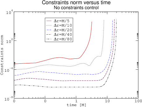
An interesting feature of the instabilities of the simulations shown in Figure 1 is that the norm growth is initially negative, but it becomes positive after a single time step, triggering the instability, see (17) (there, as in the rest of the paper, $\dot{N}_{c}$ is computed through the semidiscrete expression (3)).

$$\Delta r$$

(17)

A static choice of $\mu$ cannot account for these fluctuations. In particular, choosing $\mu$ using only the growth rate around the background solution, which in this case would be the initial data, and not the errors introduced during numerical integration, in general will not be able to correct these kind of fluctuations in $\dot{N}_{c}$.

IV.3 Strictly enforcing semidiscrete norm preservation

I now discuss some numerical experiments using a dynamically calculated $\mu(t)$ such that $\dot{N_{c}}=0$ in the semidiscrete case. For a chosen resolution, $\mu$ is defined at each time step by

$$\mu(n\Delta t)=\left\{\begin{array}[]{l}-I^{(1)}(n\Delta t)/I^{(2)}(n\Delta t)\;,\;\mbox{ if }I^{(2)}(n\Delta t)\neq 0\\ \mu\left((n-1)\Delta t\right)\;,\;\mbox{ if }I^{(2)}(n\Delta t)=0\mbox{ and }{n\geq 1}\\ 0\;,\;\;\mbox{ if }I^{(2)}(n\Delta t)=0\mbox{ and }{n=0}\end{array}\right.$$ (18)

and $\mu(n\Delta t)$ is in turn used to compute the RHS needed to advance $u\left(n\Delta t\right)$.

Figure 2: Strict conservation of the semidiscrete norm ($\dot{N}_{c}=0$), using different resolutions to define $\mu(t)$, i.e. $\mu$ is dynamically computed at each resolution. The fact that the errors increase when resolution is increased strongly suggest that defining $\mu$ this way leads to an ill-posed problem. The appropriate way of doing a convergence test is shown in Figure 3.

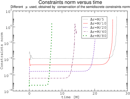
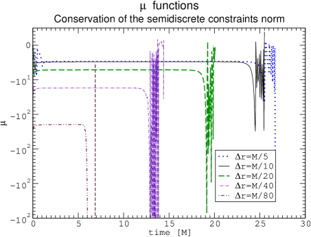
Figure 2 shows the resulting norm as a function of time, for evolutions enforcing $\dot{N}_{c}=0$ at different resolutions. The code blows up rather fast, and this happens at earlier times when resolution is increased. This last feature should not be seen as an indication of ill-posedness of the method, since Figure 2 should not be seen as a convergence test. For such a test one should dynamically define $\mu(t)$ with a given resolution and then keep that $\mu$ fixed for all other runs. Figure 3 shows the result of doing so, defining $\mu(t)$ through a run with $\Delta r=M/5$ and then keeping it fixed for a convergence test . As expected, and in contrast to Figure 2, the norm does decrease as the resolution is increased. Figure 2 strongly suggests that if one insisted in dynamically defining $\mu$ at each resolution, instead of fixing it at a single resolution, one would end up with an ill-posed problem. On the other hand, fixing $\mu$ leads to a strongly hyperbolic problem and no convergence problems appear.

Figure 3: Strict conservation of the semidiscrete norm, defining $\mu$ by a $\Delta r=M/5$ run and then fixing $\mu$ for all other runs.

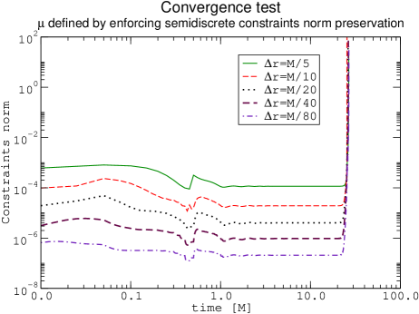
Considering these runs with $\dot{N}_{c}=0$, it appears that enforcing semidiscrete norm preservation is “too rigid” (recall the discussion at the beginning of Section III). Figure 4 shows the $\mu$ functions obtained through the runs of Figure 2. Notice that when increasing resolution the $\mu$ that is needed in order to preserve the norm increases quite fast in absolute value. For example, with $\Delta r=M/80$ the initial values of $\mu$ are of order $10^{2}$. Since $\mu$ appears in the principal part of the equations, having a large value implies the need of a small Courant factor to follow the simulation; while Figures 2 and 4, on the other hand, where obtained using the same Courant factor when changing resolution. A Fourier decomposition of the numerical solution, or an explicit von-Neumann analysis of a linear, constant coefficient problem could give further insight into this question.

A second possibility would be to perform a fully discrete analysis (as opposed to the semidiscrete one used in this paper), and to enforce strict conservation of the fully discrete norm, but these issues are not pursued here.

Figure 4: This figure shows $\mu(t)$ for the runs of Figure 2.

IV.4 Dynamically achieving a tolerance value

I now set a tolerance value $T$, and choose $\mu$ such that $N_{c}=T$ after a given number of timesteps. In doing so I use the semidiscrete expressions (8,9). If $I^{(2)}$ is zero, $\mu$ will be copied from its previous value, or set to zero if this happens in the first iteration.

Figure 5: This figure shows $\mu$ calculated by setting a tolerance value, $T=5\times 10^{-4}$, and requiring the semidiscrete norm to return to this value after every timestep. $\mu$ is defined using $\Delta r=M/5$, for which the initial, truncation value of the norm is $N_{c}=4.8\times 10^{-4}$.

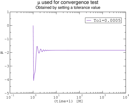
Figure 5 shows results with a dynamically defined $\mu$, using the same resolution, domain, Courant and dissipation factors as before. $n_{a}$ is chosen to be one, corresponding to the norm returning to the specified tolerance value after every time step.

The discretized constraints are, of course, not zero initially, even when the initial data is analytic, because computing them involves finite differencing the initial data. The initial value for the norm for this resolution is $N_{c}=4.8\times 10^{-4}$. Therefore I choose a tolerance value $T=5\times 10^{-4}$, to keep the constraints close to its initial value.

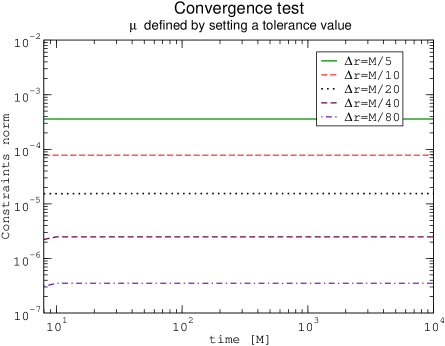
Figure 6 shows the resulting norms for a convergence test performed with the same resolutions used in Figure 1, and the $\mu$ shown in Figure 5. The code runs for $10^{4}M$ without any sign of instabilities, even with the coarse resolution that was used to define $\mu$.

Figure 6: A convergence test done with $\mu$ shown in Figure 5. Compare the lifetime of these simulations with those of Figure 1.

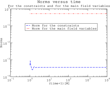
It could happen that one controls the constraints at the price of introducing other errors. This does not happen, at least in the numerical experiments here considered. In these experiments, not only does the norm associated with the constraints remains close to its initial, truncation value, but the same happens with the norm associated with the main field variables, $N=\int(a^{2}+K_{a}^{2}+K_{b}^{2})$. Since the exact solution is stationary, $N$ being close to its initial value means that the method does not introduce new errors. Figure 7 shows $N_{c}(t)$ and $N(t)$ for the run used to define $\mu$.

Figure 7: Norms associated with the constraints and with the main field variables, for the run used to obtain $\mu$ shown in Figure 5.

IV.4.1 Dependence of $\mu$ on the tolerance value

In the previous examples I chose the tolerance value, $T$, to be roughly the initial, truncation error for $N_{c}$. Although this seems the natural thing to do, I will now discuss sensitivity of the stability method with respect to the chosen value of $T$.

Figure 8: This figure shows the sensitivity of the method to the chosen tolerance value $T$. Values too large (a couple of order of magnitudes bigger than the initial truncation error $N_{c}(0)$), or smaller than $N_{c}(0)$, lead to instabilities. Otherwise, no fine tuning of $T$ is required.

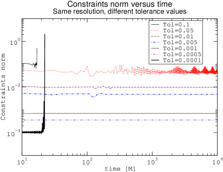
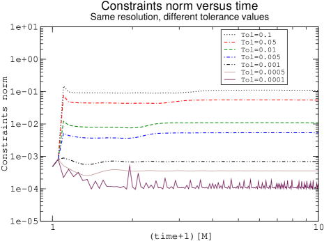
Figure 8 shows results when choosing different tolerance values to define $\mu$, but keeping all other numerical parameters (in particular, the resolution, i.e. Figure 8 is not a convergence test) fixed. When $T$ is much larger than the initial truncation value of $N_{c}$, large errors allow triggering of nonlinear instabilities. On the other hand, values of $T$ considerably smaller than the initial truncation one forces $\mu$ to change very fast, and to large values. In either case the code crashes. The $\mu$ functions for two such cases are shown in Figure 9.

Figure 9: $\mu$ for two unstable cases, with too large ($T=10^{-1}$) and too small tolerance values ($T=10^{-4}$).

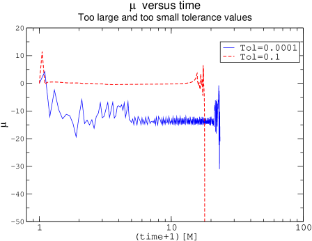
Figure 10 shows the details of Figure 8 near $t=0$. Notice that not only all the runs begin with the same (truncation) value for $N_{c}$ (this is expected, since the same resolution is used), but $N_{c}$ is also the same in the very first timestep. The reason for this is that $\mu=0$ initially for all the runs, because $I^{(2)}=0$ in the initial data. This is a coincidence of the initial data being evolved in this example: the only discretization error in the computation of the Hamiltonian constraint in this model comes from the finite differencing of $a$, which in this example is initially $1$ for all grid points.

Figure 10: The figure shows details of plot 8, near $t=0$. The norms in this experiment are the same in the initial data and first time step, as explained in the body of the paper.

IV.5 Intentional constraint violations

As a final numerical example, now I consider initial data that violates the constraints at the continuum. The equations still use the exact lapse and area-locking shift given by Eq.(16), but now the initial data are given by

$$a = \left(1+s_{1}e^{-(r-r_{0})^{2}}\right)$$ (19)

$$K_{a} = -\frac{\beta}{2r}\left(1+s_{2}e^{-(r-r_{0})^{2}}\right)$$ (20)

$$K_{b} = \frac{\beta}{r}=\left(1+s_{3}e^{-(r-r_{0})^{2}}\right)$$ (21)

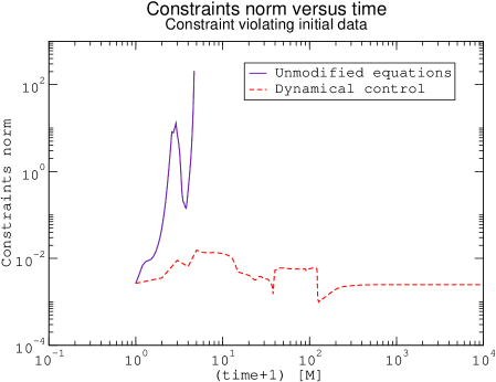
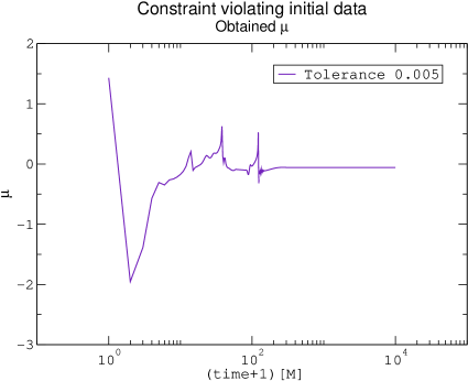
When $s_{i}=0$, this data reduces to that of the PG black hole. The constants $s_{i}$ are used to introduce an “asymmetry” in the perturbations of the PG initial data. The perturbations are rather large, with $s_{1}$ or order unity. In this example, $s_{1}=1,s_{2}=0.5,s_{3}=0.7$. When $\mu=0$ the code crashes before $t=4M$ at a resolution $\Delta r=M/5$. At this resolution $N_{c}$ for the initial data is $N_{c}(0)=2.66\times 10^{-3}$ (one order of magnitude larger than the associated truncation error for the case $s_{i}=0$, which for this resolution is $N_{c}=4.8\times 10^{-4}$ ). Thus, I choose a tolerance value of $T=5\times 10^{-3}$, $n_{1}=10$ in order to avoid fast variations, and rerun, dynamically obtaining $\mu(t)$. Results for the unmodified equations ($\mu=0$), and with a dynamical $\mu$ are shown in Figures 11, 12. The difference in stability is quite striking, especially considering that the perturbation of the PG initial data is so large.

Figure 11: The norm $N_{c}$, with and without control of the constraints, for highly perturbed initial data, at a resolution of $\Delta r=M/5$. The initial, truncation error for $N_{c}$ for this resolution is $N_{c}(0)=2.66\times 10^{-3}$, and the tolerance value is set to $T=5\times 10^{-3}$.

Figure 12: $\mu$ for the plot of Figure 11 with dynamical controlled constraints. After some time $\mu$ settles down to the value $\mu=-5.8\times 10^{-3}$.

V Remarks

There is a lot of interest in finding formulations of Einstein’s equations with good stability properties off of the constraint surface. So far, most, if not all, of the work has been concentrated in stability properties around known solutions. The purpose of this paper has been to introduce new ideas that hopefully will be helpful in generic evolutions, where one has no a priori knowledge of the solution. This is one fundamental difference with previous approaches.

Another difference is that previous work has concentrated on stability properties at the continuum. Although this is an important issue, controlling constraint violating modes introduced by the numerical method is also crucial. Thus, this proposal aims to control discrete constraint violations introduced both by the underlying formulation of equations at the continuum, and whatever numerical method one has chosen.

Sometimes it seems that one would ideally want the constraints to decay exponentially to zero lambda ,fiske . Although this might be attractive at the continuum, in what concerns the discrete constraints it might be better to maintain them around the initial, truncation error. For example, beginning with initial data corresponding to a stationary spacetime, it seems difficult to imagine that by making the constraints decrease in time through numerical integration (keeping resolution fixed), one would end up with a numerical solution that has smaller errors than the initial data, which was computed by just numerically evaluating the exact solution at given gridpoints. Thus, I have concentrated here on keeping the discrete constraints at some tolerance value, instead of forcing them to decay to zero. However, there may be other scenarios where it is preferable to make them decay to values smaller than the initial one, and the method here presented allows for this as well. Along these lines, an extension of the work presented here is to use the evolution equations applied to initial data off the constraint surface to produce solutions of the constraints as an alternative to relaxing the constraints themselves .

In some other approaches ls , a norm for the main variables, say $N(t)=\int_{S_{t}}\sum_{i}u_{i}^{2}$, is minimized with respect to constraint violating perturbations (around a given, known background). I could have here chosen to dynamically minimize this quantity. One potential problem with this is that it is not clear how much minimization makes the solution closer to the “exact” one. For example, in the spherically symmetric example here considered the time derivative of the norm for the main variables has the form

$$\dot{N}=\tilde{I^{(1)}}+\mu\tilde{I^{(2)}}$$

Since $\mu$ is completely free in this model, one is able to make $\dot{N}$, for some chosen but arbitrary resolution, as negative as one wants. What happens then is that all the field variables decay to zero (numerical experiments that I have done do confirm this). Clearly this is not what one wants, since the “exact” solution is not identically zero. On the other hand, one could also attempt to keep $N$ close to its initial, truncation value. However, this would be a good idea only if the solution is stationary, since otherwise there is no reason for the exact $N(t)$ to be close to $N(0)$ for all times. Thus I have here considered a norm associated with the constraints, since they are analytically zero, regardless of the solution.

VI Acknowledgments

I would like to thank Oscar Bruno, Gioel Calabrese, Luis Lehner, David Neilsen, Jorge Pullin, Oscar Reula, Olivier Sarbach, Ed Seidel and Jonathan Thornburg for very helpful discussions, comments and suggestions. This work was supported in part by NSF grant PHY9800973, the Horace Hearne Jr. Institute for Theoretical Physics, and Fundación Antorchas.

References

- (1) G. Calabrese and O. Sarbach, gr-qc/0303040; B. Szilagyi and J. Winicour, gr-qc/0205044; B. Szilagyi, B. Schmidt, and J. Winicour, Phys. Rev. D 65, 064015 (2002); G. Calabrese, J. Pullin, O. Reula, O. Sarbach, and M. Tiglio, gr-qc/0209017, to appear in Communications in Mathematical Physics; G. Calabrese, L. Lehner, and M. Tiglio, Phys. Rev. D 65, 104031 (2002); J. M. Stewart, Class. Quantum Grav. 15, 2865 (1998).
- (2) G. Calabrese, L. Lehner, D. Neilsen, J. Pullin, O. Reula, O. Sarbach, and M. Tiglio gr-qc/0302072; “Summation by parts and dissipation for black hole excision”, in preparation.
- (3) D. Fiske, gr-qc/0304024.
- (4) H. Friedrich and A. Rendall, in Einstein’s Field Equations and their Physical Implications, Lecture Notes in Physics, edited by B. G. Schmidt (Springer Verlag, Berlin, 2000), p. 127-223; O. Reula, Living Rev. Rel. 1, 3 (1998).
- (5) T. Baumgarte and S. Shapiro, Phys. Rept. 376, 41 (2003); L. Lehner, Class. Quant. Grav. 18, R25 (2001).
- (6) O. Sarbach and M. Tiglio; Phys. Rev. D 66, 064023 (2002).
- (7) B. Kelly, P. Laguna, K. Lockitch, J. Pullin, E. Schnetter, D. Shoemaker, and M. Tiglio, Phys. Rev. D 64, 084013 (2001); L. Lehner, M. Huq, M. Anderson, E. Bonning, D. Schaefer, R. Matzner, Phys. Rev. D 62, 044037 (2000); D. Garfinkle and C. Gundlach, Class. Quant. Grav. 16, 4111 (1999).
- (8) O. Brodbeck, S. Frittelli, P. Hubner, and O. Reula, J. Math. Phys. 40, 909 (1999); S. Detweiler, Phys. Rev. D 35, 1095 (1987).
- (9) L. Lindblom and M. Scheel, Phys. Rev. D 66, 084014 (2002).