Microcausality and Quantum Cylindrical Gravitational Waves

Abstract

We study several issues related to the different choices of time available for the classical and quantum treatment of linearly polarized cylindrical gravitational waves. We pay especial attention to the time evolution of creation and annihilation operators and the definition of Fock spaces for the different choices of time involved. We discuss also the issue of microcausality and the use of field commutators to extract information about the causal properties of quantum spacetime.

I Introduction

The quantization of polarized gravitational cylindrical waves has received a lot of attention in recent years Ashtekar (1996); Ashtekar and Pierri (1996); Angulo and Mena Marugan (2000); Gambini and Pullin (1997); Dominguez and Tiglio (1999); Varadarajan (2000); Cruz, Miković and Navarro-Salas (1998); Romano and Torre (1996); Korotkin (1998). This is partly due to the fact that this system provides a tractable, yet non-trivial, reduction of full general relativity and hence is an ideal framework to explore several issues involved in the quantization of gravity. Some intriguing phenomena, related to the existence of large quantum gravity effects, have been discussed by studying precisely this model Ashtekar (1996); Ashtekar and Pierri (1996); Angulo and Mena Marugan (2000); Gambini and Pullin (1997); Dominguez and Tiglio (1999). It has also been argued that some manifestations of quantum gravity, such as the smearing of light cones are, indeed, present and can be understood in this simplified setting Ashtekar and Pierri (1996).

One of the interesting points behind the obtained results is the realization of the fact that the physical Hamiltonian is a function of the free field Hamiltonian for a 2+1 dimensional, axially symmetric, massless scalar field evolving in an auxiliary Minkowski background Ashtekar (1996); Kuchař (1971); Ashtekar, Bičák and Schmidt (1997). As we show in the first section of the paper, this free Hamiltonian naturally appears when one linearizes the system, thus suggesting that, in a precise sense, it can be considered as the free part of an interacting model. However the full interacting Hamiltonian is obtained by adding a very specific type of terms to the free part, namely, just functions of it. Here we plan to explore the consequences of this functional relation between the two physically relevant Hamiltonians for the system and explore how this affects the causal structure of quantum spacetime. To this end we will pay attention to the smearing of the light cones due to quantum gravity effects within the framework of linearly polarized cylindrical waves. Instead of considering the full information encoded in the metric tensor we will concentrate on the causal structure provided by light cones. An interesting, albeit somewhat indirect way, to look at this structure is to study the commutators of field operators at different spacetime points. These are the basic objects to discuss the commutativity of observables and the microcausality of the model; conventionally, a physical model should be such that observables commute for space-like intervals. This has been discussed in the standard perturbative quantum field theory framework for simple examples such as scalar or fermion fields (see e.g. Peskin (1995)). In fact, microcausality is one of the key conditions to prove such important results as the spin-statistics theorem Peskin (1995); Pauli (1940).

Here we will use the commutator of the scalar field that describes linearly polarized cylindrical waves as a way to get information about the causal structure of quantum spacetime. As we show later it is possible to give exact expressions for this commutator both for the evolution provided by the free and the full physical Hamiltonians. We will use these expressions to study in a quantitative way the smearing of the light cones as a function of the three-dimensional gravitational constant and explore some physical issues, in particular the appearance of singularities as a consequence of having a Hamiltonian bounded from above Ashtekar and Varadarajan (1994); Varadarajan (1995).

The rest of the paper is structured as follows. In Sec. II we discuss how the free Hamiltonian is derived from the linearized cylindrical wave model. Sec. III deals with the classical and quantum dynamics of cylindrical gravitational waves under the evolution provided both by the free Hamiltonian and the physical Hamiltonian. We will pause here to discuss and compare on a familiar example (the harmonic oscillator) the main features of the time evolution defined by functionally related Hamiltonians, both from the classical and the quantum points of view. This will provide valuable insights for the problem considered in this work. Sec. IV is devoted to the study of microcausality. We will look at the main features of the field commutators and study the smearing of the light cones due to quantum gravitational effects. We end the paper with a discussion of the main results and perspectives for future work.

II Cylindrical Waves in Linearized Gravity

Linearly polarized cylindrical waves in general relativity can be described by the spacetime metric Ashtekar and Pierri (1996); Angulo and Mena Marugan (2000):

$$ds^{2}=e^{-\psi}ds_{3}^{2}+e^{\psi}dZ^{2},$$ (1)

where $Z\in\mathbb{R}$ is the coordinate of the symmetry axis and $ds_{3}^{2}$ is the three-metric

$$ds_{3}^{2}=-N^{2}dt^{2}+e^{\gamma}(dR+N^{R}dt)^{2}+r^{2}d\theta^{2}.$$ (2)

From this three-dimensional point of view, $R\in\mathbb{R}^{+}$ and $\theta\in S^{1}$ correspond to polar coordinates, $N^{R}$ is the radial component of the shift vector and $N$ is the lapse function. All metric functions ($\gamma$, $r$, $N$, and $N^{R}$) depend only on the time and radial coordinates, $t$ and $R$.

Unless otherwise stated, we adopt a system of units such that $c=\hbar=8G_{3}=1$, where $c$ is the speed of light, $\hbar$ is Planck constant, and $G_{3}$ is the effective Newton constant per unit length in the direction of the symmetry axis Angulo and Mena Marugan (2000). In these units, the gravitational action of the system has the form Kuchař (1971); Romano and Torre (1996)

$$S=\int_{t_{1}}^{t_{2}}dt\left[\int_{0}^{\infty}dR\,(p_{\gamma}\dot{\gamma\;}+p_{r}\dot{r}+p_{\psi}\dot{\psi})-{\cal H}\right],$$ (3)

where the dot denotes the derivative with respect to $t$, the $p$’s are the momenta canonically conjugate to the metric variables and $\cal{H}$ is the total Hamiltonian

$${\cal H}=2\left(1-e^{-\gamma_{\infty}/2}\right)+\int_{0}^{\infty}dR\left[NC+N^{R}C^{R}\right].$$ (4)

The first term is a boundary contribution at infinity [$\gamma_{\infty}:=\gamma(R\rightarrow\infty)$] and the second term is a linear combination of the Hamiltonian constraint $C$ and the (radial) diffeomorphisms constraint $C^{R}$:

$$C\; = e^{-\gamma/2}\left[2r^{\,\prime\prime}-\gamma^{\prime}r^{\>\prime}-p_{\gamma}p_{r}+\frac{p_{\psi}^{2}}{2r}+\frac{r(\psi^{\prime})^{2}}{2}\right],$$

$$C^{R} = e^{-\gamma}\left(-2p^{\prime}_{\gamma}+p_{\gamma}\gamma^{\prime}+p_{r}r^{\>\prime}+p_{\psi}\psi^{\prime}\right).$$

The prime denotes the derivative with respect to $R$. The gauge freedom associated with these constraints can be removed by imposing, respectively, the gauge fixing conditions Ashtekar and Pierri (1996); Angulo and Mena Marugan (2000)

$$\chi^{R}:=r-R=0,\hskip 17.07182pt\chi\,:=p_{\gamma}=0.$$

On the other hand, the Lagrangian form of the action can be obtained from the relations between momenta and time derivatives of the metric provided by the Hamilton equations,

$$p_{\gamma}N = -e^{\gamma/2}\dot{r}+e^{-\gamma/2}N^{R}r^{\>\prime},$$

$$p_{\psi}N = e^{\gamma/2}r\,\dot{\psi}-e^{-\gamma/2}N^{R}r\,\psi^{\prime},$$

$$p_{r}N = -e^{\gamma/2}\dot{\gamma\,}+2\left(N^{R}e^{-\gamma/2}\right)^{\prime}.$$

From a three-dimensional perspective, the system describes an axially symmetric model consisting of a scalar field $\psi$ coupled to gravity Ashtekar and Pierri (1996), the line element being (2). A particular classical solution is a vanishing scalar field in three-dimensional Minkowski spacetime or, equivalently, Minkowski spacetime in four dimensions. In this solution, $N=1$ and $r=R$, whereas the rest of metric fields and momenta vanish (i.e. $\psi=\gamma=N^{R}=p_{\psi}=p_{\gamma}=p_{r}=0$).

In this section, we will consider this solution as a background and discuss first-order perturbations around it. In other words, we will analyze the linearized theory of gravity around this Minkowski spacetime, as it is usually done in the perturbative, quantum field theory approach to gravity. In order to expand the metric fields around the classical solution, let us call

$$r=R+\bar{r},\hskip 17.07182ptN=1+\bar{N}.$$

Up to first-order terms in the fields, the expression of the three-metric becomes

$$d\bar{s}_{3}^{2} = -(1+2\bar{N})dt^{2}+2N^{R}dtdR+(1+\gamma)dR^{2}$$

$$+(R^{2}+2R\bar{r})d\theta^{2},$$

while the four-dimensional metric is given by

$$d\bar{s}^{2}=(1-\psi)d\bar{s}_{3}^{2}+(1+\psi)dZ^{2}.$$ (5)

Here, it is understood that the product of $\psi$ with any other metric field vanishes in the perturbative order considered. On the other hand, regularity on the axis of symmetry imposes the following conditions:

$$\gamma(R=0) = 0,\hskip 17.07182ptN^{R}(R=0)=0,$$

$$\bar{r}(R=0) = 0,\hskip 17.07182pt\bar{r}^{\,\prime}(R=0)=0.$$ (6)

In order to discuss the linearized gravitational system, we must keep up to quadratic terms in the fields in the action (3). A straightforward calculation leads to the result

$$\bar{S} = \int_{t_{1}}^{t_{2}}dt\left[\int_{0}^{\infty}dR\,(p_{\gamma}\dot{\gamma\;}+p_{\bar{r}}\dot{\bar{r}\;}+p_{\psi}\dot{\psi})-\bar{\cal H}\right],$$

$$\bar{\cal H} = \int_{0}^{\infty}dR\left[\frac{p_{\psi}^{2}}{2R}+\frac{R\,(\psi^{\prime})^{2}}{2}-p_{\gamma}p_{\bar{r}}+\bar{N}\bar{C}+N^{R}\bar{C}^{R}\right]$$

$$+(2-\gamma_{\infty})\,\bar{r}^{\,\prime}(R\rightarrow\infty).$$

Here, $p_{\bar{r}}:=p_{r}$ is the momentum canonically conjugate to $\bar{r}$, and the linearized constraints are:

$$\bar{C}=2\bar{r}^{\,\prime\prime}-\gamma^{\prime},\hskip 17.07182pt\bar{C}^{R}=p_{\bar{r}}-2p_{\gamma}^{\prime}.$$

The diffeomorphisms gauge freedom can be fixed just like in the cylindrical reduction of general relativity, namely, by demanding that $r=R+\bar{r}$ coincides with the radial coordinate Angulo and Mena Marugan (2000). We thus impose the gauge fixing condition $\bar{\chi}^{R}:=\bar{r}=0$. It is easily checked that the Poisson brackets $\{\bar{\chi}^{R},\bar{C}^{R}\}$ of this condition with the linearized constraint do not vanish, so that the gauge fixing is admissible. Dynamical consistency of the gauge fixing procedure requires, in addition,

$$\dot{\;\bar{\chi}^{R}}=\{\bar{\chi}^{R},\bar{\cal H}\}=N^{R}-p_{\gamma}=0.$$

Hence, the shift must be chosen as $N^{R}=p_{\gamma}$. Finally, the momentum conjugate to $\bar{r}$ is fixed by solving the diffeomorphisms constraint: $p_{\bar{r}}=2p_{\gamma}^{\prime}$. In this way, the canonical pair $(\bar{r},p_{\bar{r}})$ is removed from the set of degrees of freedom. The action of the resulting reduced model is

$$\bar{S}_{1} = \int_{t_{1}}^{t_{2}}dt\int_{0}^{\infty}dR\,\left(p_{\gamma}\dot{\gamma\;}+p_{\psi}\dot{\psi}-\bar{N}\bar{C}_{1}\right)$$

$$- \int_{t_{1}}^{t_{2}}dt\left[H_{0}-p_{\gamma}^{2}(R\rightarrow\infty)+p_{\gamma}^{2}(R=0)\right].$$

Here, $\bar{C}_{1}=-\gamma^{\prime}$ is the Hamiltonian constraint of the reduced linearized system, and

$$H_{0}=\int_{0}^{\infty}dR\left[\frac{p_{\psi}^{2}}{2R}+\frac{R\,(\psi^{\prime})^{2}}{2}\right].$$ (7)

Remarkably, the condition employed to eliminate the Hamiltonian gauge freedom in full cylindrical gravity Angulo and Mena Marugan (2000) can be used as well to fix the corresponding gauge in the linearized theory. The gauge fixing $\bar{\chi}\,:=p_{\gamma}=0$ is acceptable, because the Poisson brackets of $\bar{\chi}$ and $\bar{C}_{1}$ differ from zero. In addition, consistency of the chosen gauge demands the vanishing of

$$\dot{\bar{\chi}\,}=\left\{\bar{\chi}\;,\;H_{0}+\!\int_{0}^{\infty}\!\!dR\,\bar{N}\bar{C}_{1}\right\}=-\bar{N}^{\prime}.$$

Therefore, $\bar{N}$ has to be independent of the radial coordinate. Actually, we can set $\bar{N}=0$ by demanding that the total lapse equals the unity at spatial infinity. On the other hand, taking into account the regularity condition (II), the solution to the Hamiltonian constraint is simply $\gamma=0$. This allows us to remove the canonical pair $(\gamma,p_{\gamma})$ from the system and arrive at a constraint-free model in linearized gravity.

The degrees of freedom of this system are the field $\psi$ and its momentum. The reduced action is

$$\bar{S}_{2}=\int_{t_{1}}^{t_{2}}dt\left[-H_{0}+\int_{0}^{\infty}\!dR\;p_{\psi}\dot{\psi}\right].$$

Note that $H_{0}$, given in Eq. (7), is the Hamiltonian of a massless scalar field with axial symmetry in three-dimensions. Furthermore, in the gauge that we have selected, the three-dimensional metric of the linearized gravitational theory is exactly that of Minkowski spacetime and contains no physical degrees of freedom. The scalar field $\psi$ determines the norm of the Killing vector $\partial_{Z}$, and appears in the four-dimensional metric of the gauge-fixed, linearized model in the form (5), but with $d\bar{s}_{3}^{2}$ substituted by the flat metric

$$\left(d\bar{s}_{3}^{2}\right)_{f}:=-dT^{2}+dR^{2}+R^{2}d\theta^{2},$$ (8)

where we have renamed $T$ the time coordinate of the reduced system.

Summarizing, the perturbative description provided in linearized gravity for cylindrical waves with linear polarization around four-dimensional Minkowski spacetime is equivalent to a massless scalar field with axial symmetry in a three-dimensional flat background. The dynamics of this field is dictated by the free Hamiltonian $H_{0}$, which generates the evolution in the Minkowskian time $T$.

It is worth noticing that the action and metric of the gauge-fixed model in linearized gravity reproduce in fact the results that one would obtain from the gauge-fixed model in full cylindrical gravity by working just in the first perturbative order, i.e., by keeping in the action and metric, respectively, up to quadratic and linear terms in the field $\psi$ and its momentum. In this sense, the gauge fixing and linearization procedures commute.

III Time Coordinates and Evolution for Cylindrical Waves

III.1 Systems with Functionally Related Hamiltonians

One of the significant features of gravitational cylindrical waves is the existence of two distinct, physically relevant Hamiltonians (or equivalently two distinct time coordinates) to define both the classical and quantum evolution. One is the Hamiltonian $H_{0}$ [given in Eq. (7)] that generates the dynamics in the linearized gravitational theory; the other is the Hamiltonian $H$ that provides the energy per unit length along the symmetry axis in general relativity Ashtekar and Varadarajan (1994); Varadarajan (1995); Ashtekar and Pierri (1996). In fact, they are functionally dependent, since $H=2(1-e^{-H_{0}/2})$. In order to gain insight into the relation that can be established between the dynamics associated with these two different Hamiltonians, we open this section by discussing a similar situation in a very simple example provided by the harmonic oscillator.

The usual description of the harmonic oscillator in a phase space coordinatized by $(x_{0},p_{0})$ comes from its standard Hamiltonian $h_{0}(x_{0},p_{0})=(p^{2}_{0}+\omega^{2}x^{2}_{0})/2$. The dynamics is given by the Hamilton equations

$$\frac{dx_{0}}{dT}=p_{0}\,,\quad\frac{dp_{0}}{dT}=-w^{2}x_{0}\,.$$

The general solution can be written as

$$x_{0}(T) = \frac{1}{\sqrt{2\omega}}\left(ae^{-i\omega T}+a^{\dagger}e^{i\omega T}\right),$$

$$p_{0}(T) = \frac{-i\omega}{\sqrt{2\omega}}\left(ae^{-i\omega T}-a^{\dagger}e^{i\omega T}\right),$$

where $a$ and its complex conjugate $a^{\dagger}$ are fixed by the initial conditions.

Consider next a phase space $(x,p)$ with Hamiltonian $h=F(h_{0})$, i.e. a function of the standard Hamiltonian for the harmonic oscillator. For instance, the case $F(h_{o})=h_{0}^{2}$ arises in the context of quantum optics, in relation with the propagation of light in non-linear Kerr media Leoński (1998). The equations of motion now read

$$\frac{dx}{dt} = \{x,F(h_{0})\}=F^{\prime}(h_{0})p\,,$$

$$\frac{dp}{dt} = \{p,F(h_{0})\}=-\omega^{2}F^{\prime}(h_{0})x\,,$$

where $F^{\prime}$ denotes the derivative of $F$ with respect to its argument. These new equations can be easily solved by means of a change of time. Specifically, making use of the time independence of the Hamiltonian $h_{0}$ ($h_{0}=wa^{\dagger}a$ on solutions to the equations of motion), we can introduce the new time parameter $T(t)=F^{\prime}(h_{0})t$. Then, the functions $x(t)=x_{0}[T(t)]$, $p(t)=p_{0}[T(t)]$ and the new time $T$ serve us to transform the Hamilton equations into the standard ones corresponding to the harmonic oscillator. So, the classical solutions are

$$x(t)\!=\!x_{0}[T(t)]\!=\!\frac{1}{\sqrt{2\omega}}\!\left[ae^{\!-i\omega F^{\prime}(\omega a^{\dagger}\!a)t}\!+\!a^{\dagger}e^{i\omega F^{\prime}(\omega a^{\dagger}\!a)t}\right]\!,$$

$$p(t)\!=\!p_{0}[T(t)]\!=\!\frac{-i\omega}{\sqrt{2\omega}}\!\left[ae^{\!-i\omega F^{\prime}(\omega a^{\dagger}\!a)t}\!-a^{\dagger}e^{i\omega F^{\prime}(\omega a^{\dagger}\!a)t}\right]\!.$$

What we find is an energy dependent redefinition of time that induces a different time change for each solution to the equations of motion.

The situation in the quantum theory is quite different. The reason lies on the fact than in quantum mechanics a physical state does not need to have a definite energy. Then, a “change of time” of the form $\hat{T}=F^{\prime}(\hat{h}_{0})t$ has non-trivial consequences for the dynamics.

The usual quantum theory for the harmonic oscillator can be described by introducing a Fock space with creation and annihilation operators $a^{\dagger}$, $a$. Every initial state can be expressed as $|\phi(0)\rangle=\sum_{n=0}^{\infty}c_{n}|n\rangle$, where $c_{n}$ are Fourier coefficients (with the convenient normalization) and $|n\rangle$ are energy eigenvectors (that is, $\hat{h}_{0}|n\rangle=nw|n\rangle$). In the Schrödinger picture, evolving with $\hat{h}_{0}$, we find

$$|\phi_{0}(T)\rangle = e^{-i\hat{h}_{0}T}|\phi(0)\rangle=\sum_{n=0}^{\infty}c_{n}e^{-inwT}|n\rangle\,.$$

However, if the same state $|\phi(0)\rangle$ evolves in time according to the evolution generated by $\hat{h}=F(\hat{h}_{0})$, we get

$$|\phi_{F}(t)\rangle = e^{-i\hat{h}t}|\phi(0)\rangle=\sum_{n=0}^{\infty}c_{n}e^{-iF(nw)t}|n\rangle\,.$$

Hence we do not recover an analogous situation to that found in the classical system by replacing (formally) the time $T$ in $|\phi_{0}(T)\rangle$ with $\hat{T}=F^{\prime}(\hat{h}_{0})t$, because $|\phi_{F}(t)\rangle\neq|\phi_{0}(\hat{T}(t))\rangle$ except for linear homogeneous functions $F$. Moreover, the properties of the states $|\phi_{0}(T)\rangle$ and $|\phi_{F}(t)\rangle$ are quite different. For example, if we consider the bounded Hamiltonian $\hat{h}=F(\hat{h}_{0})=1-e^{-\hat{h}_{0}}$ it is obvious that the high energy contributions to $|\phi_{F}(t)\rangle$ are essentially frozen in time with respect to the evolution of the low energy ones, in the sense that the phase of the former type of contributions remains practically coherent in time.

III.2 Functionally Related Hamiltonians and Cylindrical Waves

Let us turn now to the discussion of our gravitational system. We will deal with the Einstein-Rosen family of linearly polarized gravitational waves Einstein and Rosen (1937). These waves display the so-called whole cylindrical symmetry Melvin (1965), namely, they correspond to topologically trivial spacetimes which possess two linearly independent, commuting, spacelike, and hypersurface orthogonal Killing vector fields. It is well known Kuchař (1971); Romano and Torre (1996) that these spacetimes admit coordinates $(T,R,\theta,Z)$ such that the metric is given by

$$ds^{2}=e^{\gamma-\psi}(-dT^{2}+dR^{2})+e^{-\psi}R^{2}d\theta^{2}+e^{\psi}dZ^{2},$$

where $\psi$ and $\gamma$ are functions of only $R$ and $T$. When the Einstein equations are imposed, $\psi$ encodes the physical degrees of freedom and satisfies the usual wave equation for an axially symmetric massless scalar field in three-dimensions:

$$\partial_{T}^{2}\psi-\partial_{R}^{2}\psi-\frac{1}{R}\partial_{R}\psi=0\,.$$

The metric function $\gamma$ can be expressed in terms of this field on the classical solutions Ashtekar and Pierri (1996); Angulo and Mena Marugan (2000). One gets

$$\gamma(R) = \frac{1}{2}\int^{R}_{0}d\bar{R}\,\bar{R}\,\left[(\partial_{T}\psi)^{2}+(\partial_{\bar{R}}\psi)^{2}\right],$$

$$\gamma_{\infty} = \frac{1}{2}\int^{\infty}_{0}dR\,R\,\left[(\partial_{T}\psi)^{2}+(\partial_{R}\psi)^{2}\right].$$ (9)

Note that $\gamma(R)$ and $\gamma_{\infty}$ are the energy of the scalar field in a ball of radius $R$ and in the whole of the two-dimensional flat space, respectively. Furthermore, $\gamma_{\infty}$ coincides with the Hamiltonian $H_{0}$ given in Eq. (7) Ashtekar and Pierri (1996).

Nevertheless, to reach a unit asymptotic timelike Killing vector field in the actual four-dimensional spacetime, with respect to which one can truly introduce a physical notion of energy (per unit length) Ashtekar and Varadarajan (1994); Varadarajan (1995), one must make use of a different system of coordinates, namely $(t,R,\theta,Z)$ where $T=e^{-\gamma_{\infty}/2}t$. In these new coordinates the metric has the form

$$ds^{2}=e^{\gamma-\psi}(-e^{-\gamma_{\infty}}dt^{2}+dR^{2})+e^{-\psi}R^{2}d\theta^{2}+e^{\psi}dZ^{2}.$$

Assuming as a boundary condition that the metric function $\psi$ falls off sufficiently fast as $R\rightarrow\infty$, the above metric describes asymptotically flat spacetimes with a, generally non-zero, deficit angle. In this asymptotic region $\partial_{t}$ is a unit timelike vector. The Einstein field equations can be obtained from a Hamiltonian action principle Ashtekar and Varadarajan (1994); Varadarajan (1995); Romano and Torre (1996) where the on-shell Hamiltonian is given in terms of that for the free scalar field by

$$H=E(H_{0})=2(1-e^{-H_{0}/2}).$$ (10)

Owing to these reasons, in the following we will refer to $t$ as the physical time and to $H$ as the physical Hamiltonian.

When we use the $T$-time and impose regularity at the origin $R=0$ Ashtekar and Pierri (1996), the classical solutions for the field $\psi$ can be expanded in the form

$$\psi(R,T)=\int_{0}^{\infty}\!\!\frac{dk}{\sqrt{2}}\,J_{0}(Rk)\left[A(k)e^{-ikT}+A^{\dagger}(k)e^{ikT}\right].$$

$A(k)$ and $A^{\dagger}(k)$ are fixed by the initial conditions and are complex conjugate to each other, because $\psi$ and $J_{0}$ (the zeroth-order Bessel function of the first kind) are real. From Eq. (9), we then obtain

$$\gamma_{\infty}=H_{0}=\int_{0}^{\infty}dk\,kA^{\dagger}(k)A(k).$$

Using this formula, we can express the field in the $t$-frame as

$$\psi_{E}(R,t)=\hskip 182.09746pt$$

$$\int_{0}^{\infty}\!\!\frac{dk}{\sqrt{2}}\,J_{0}(Rk)\left[A(k)e^{-ikte^{-\gamma_{\infty}/2}}\!+\!A^{\dagger}(k)e^{ikte^{-\gamma_{\infty}/2}}\right].\;$$

Notice that $\psi(R,0)=\psi_{E}(R,0)$.

In principle, the quantization of the field $\psi$ can be carried out in a standard way. We can introduce a Fock space in which $\hat{\psi}(R,0)$, the quantum counterpart of $\psi(R,0)$, is an operator-valued distribution Reed and Simon (1975). Its action is determined by those of $\hat{A}(k)$ and $\hat{A}^{\dagger}(k)$, the usual annihilation and creation operators, whose only non-vanishing commutators are

$$\left[\hat{A}(k_{1}),\hat{A}^{\dagger}(k_{2})\right]=\delta(k_{1},k_{2}).$$ (11)

Explicitly,

$$\hat{\psi}(R,0)\!=\!\hat{\psi}_{E}(R,0)\!=\!\!\!\int_{0}^{\infty}\!\!\!\frac{dk}{\sqrt{2}}\,J_{0}(Rk)\!\left[\hat{A}(k)\!+\!\hat{A}^{\dagger}(k)\right]\!.$$ (12)

In the Schrödinger picture, operators do not evolve, and the problem of the time evolution is transferred to the physical states. We will return later to this issue. In the Heisenberg picture, on the contrary, operators change in time and states remain fixed. In this case, the value of the quantum field $\hat{\psi}$ at any time can be obtained from its value at $T=t=0$, evolving in one of the two times that we have at hand. One is the physical time $t$, with associated Hamiltonian $H$ given in Eq. (10). The other is the time $T$ of the auxiliary three-dimensional Minkowski spacetime, its Hamiltonian being that of a massless scalar field, $H_{0}$. From our discussion in Sec. II, this time can be identified with the perturbative time (denoted also by $T$) that arises in the study of the Einstein-Rosen waves in linearized gravity.

In the perturbative time $T$, the evolution is provided by the unitary operator $\hat{U}_{0}(T)=\exp(-iT\hat{H}_{0})$ where

$$\hat{H}_{0}=\int^{\infty}_{0}dk\,k\,\hat{A}^{\dagger}(k)\hat{A}(k)$$ (13)

is the quantum Hamiltonian of an axially symmetric scalar field in three dimensions. Then

$$\hat{\psi}(R,T)\!\!\! = \!\hat{U}^{\dagger}_{0}(T)\Psi(R,0)\hat{U}_{0}(T)$$

$$= \!\!\!\!\int_{0}^{\infty}\!\!\frac{dk}{\sqrt{2}}\,J_{0}(Rk)\!\left[\hat{A}(k)e^{-ikT}\!+\!\hat{A}^{\dagger}(k)e^{ikT}\right]\!.\hskip 8.5359pt$$ (14)

The quantization procedure in this case is very simple: we have substituted the initial conditions $A(k)$ and $A^{\dagger}(k)$ in the classical solution by the corresponding quantum operators.

The situation changes when we choose the physical time $t$ as the time parameter. The quantum Hamiltonian can be defined as $\hat{H}=E(\hat{H}_{0})=2(1-e^{-\hat{H}_{0}/2})$. We can then reach a unitary evolution by means of $\hat{U}(t)=\exp(-it\hat{H})$. This leads to the following time evolved operators

$$\hat{A}_{E}(k,t)\!\! := \!\!\hat{U}^{\dagger}(t)\hat{A}(k)\hat{U}(t)=\exp\!\left[-itE(k)e^{-\hat{H}_{0}/2}\right]\!\hat{A}(k),$$

$$\hat{A}_{E}^{\dagger}(k,t)\!\! = \!\hat{A}^{\dagger}(k)\,\exp\!\left[itE(k)e^{-\hat{H}_{0}/2}\right],$$ (15)

where $E(k)=2(1-e^{-k/2})$. It is important to realize that the quantum evolution in the physical $t$-frame is not obtained by changing $A(k)$, $A^{\dagger}(k)$, and $\gamma_{\infty}$ by their direct quantum counterparts. In fact, by restoring the value of the dimensionful constants $\hbar$ and $G_{3}$, we can write $E(k)=(1-e^{-4\bar{G}k})/(4G_{3})$ with $\bar{G}=\hbar G_{3}$, so that

$$\frac{t}{\hbar}E(k)=tk+o(\hbar),$$

and we can expand $\hat{A}_{E}(k,t)$ and $\hat{A}_{E}^{\dagger}(k,t)$ in powers of $\hbar$,

$$\hat{A}_{E}(k,t) = \exp\left(-itke^{-4\bar{G}\hat{H}_{0}}\right)\hat{A}(k)+o(\hbar),$$

$$\hat{A}_{E}^{\dagger}(k,t) = \hat{A}^{\dagger}(k)\exp\left(itke^{-4\bar{G}\hat{H}_{0}}\right)+o(\hbar).$$

(Here, we have expressed $\hat{H}_{0}$ with dimensions of an inverse length)

Setting again $8\bar{G}=1$, the expansion above clearly shows that the quantum evolution of the creation and annihilation variables in the physical time differs from the “classical evolution” in higher-order quantum corrections.

This unusual behavior can be partially corrected in the sense that one can actually find an operator for $H$ such that the quantum evolution in the $t$-time is similar to the classical one. In fact, if one considers the normal ordered Hamiltonian $\hat{H}_{nor}=:\hat{H}:$ and its associated unitary evolution operator $\hat{U}_{nor}=\exp(-it\hat{H}_{nor})$, it is easy to prove that

$$\hat{A}_{nor}(k,t) = \!\exp\left(-itk:e^{-\hat{H}_{0}/2}:\right)\hat{A}(k),$$

$$\hat{A}^{\dagger}_{nor}(k,t) = \!\hat{A}^{\dagger}(k)\exp\left(itk:e^{\hat{H}_{0}/2}:\right).$$

Therefore, the quantum evolution in $t$ given by $\hat{H}_{nor}$ parallels that encountered in the classical picture. Unfortunately, there is a severe problem with this quantum dynamics that renders it physically unacceptable: the Hamiltonian $\hat{H}_{nor}$ is unbounded both from above and below Ashtekar and Pierri (1996).

Obviously, the different possibilities for the unitary time evolution of the field $\hat{\psi}$ considered here are closely related. Specifically, there exists a unitary mapping between both types of evolution. This is a consequence of the fact that they are both unitary and coincide with the identity in the same Hilbert space at $T=t=0$. So, if we denote the operators evolved from $\hat{X}(0)$ in the times $T$ and $t$ by $\hat{X}(T)=\hat{U}_{0}^{\dagger}(T)\hat{X}(0)\hat{U}_{0}(T)$ and $\hat{X}_{E}(t)=\hat{U}^{\dagger}(t)\hat{X}(0)\hat{U}(t)$, respectively, we obtain

$$\hat{X}_{E}(t)=\hat{U}^{\dagger}(t)\hat{U}_{0}(T)\hat{X}(T)\hat{U}^{\dagger}_{0}(T)\hat{U}(t)\,.$$

Then, we can go from one evolution to the other by means of the unitary operator $\hat{U}^{\dagger}_{0}(T)\hat{U}(t)$.

Let us close this section with a few comments about the Fock space on which the field $\hat{\psi}$ acts. In the Heisenberg picture the states do not depend on time. They are constructed by successive actions of the time independent creation operators on the vacuum of the theory. It is important to point out that both $\hat{H}_{0}$ and $\hat{H}$ act on the same Hilbert space and have the same vacuum, that will be referred to as $|0\rangle$. Explicitly, given any square integrable complex function $\phi_{n}(k_{1},\dots,k_{n})$ (with the convenient normalization) we can write a $n$-particle state in the form

$$|\phi_{n}\rangle\!=\!\!\!\int_{0}^{\infty}dk_{1}\cdots\int_{0}^{\infty}dk_{n}\phi_{n}(k_{1},\dots,k_{n})\hat{A}^{\dagger}(k_{1})\cdots\hat{A}^{\dagger}(k_{n})|0\rangle.$$

According to the usual interpretation of quantum mechanics, the measurable physical quantities correspond to expectation values of observables. We can go over to the Schrödinger picture by assigning the time evolution to the quantum states

$$X(t;\phi)\!=\!\langle\phi(0)|\hat{U}^{\dagger}\!(t)\hat{X}(0)\hat{U}\!(t)|\phi(0)\rangle\!=\!\!\langle\phi(t)|\hat{X}(0)|\phi(t)\rangle.$$

Defining $|\phi_{E}(t)\rangle=\hat{U}(t)|\phi(0)\rangle$, $|\phi(T)\rangle=\hat{U}_{0}(T)|\phi(0)\rangle$, and noticing that the $U$-operators satisfy

$$i\partial_{t}\hat{U}(t)=\hat{H}\hat{U}(t),\quad\quad i\partial_{T}\hat{U}_{0}(T)=\hat{H}_{0}\hat{U}_{0}(T)\,,$$

it is straightforward to see that the evolved states are solutions to the Schrödinger equations

$$i\partial_{t}|\phi_{E}(t)\rangle=\hat{H}|\phi_{E}(t)\rangle,\quad\quad i\partial_{T}|\phi(T)\rangle=\hat{H}_{0}|\phi(T)\rangle\,.$$

As in the Heisenberg picture, the unitary operator $\hat{U}(t)\hat{U}^{\dagger}_{0}(T)$ provides the bridge between the two kinds of quantum evolution,

$$|\phi_{E}(t)\rangle=\hat{U}(t)\hat{U}^{\dagger}_{0}(T)|\phi(T)\rangle\,.$$

Particularizing the above results to the case of $n$-particle states we readily get that, for the $T$-time,

$$|\phi_{n}(T)\rangle=\hat{U}_{0}(T)|\phi_{n}\rangle=\hskip 125.19194pt$$

$$\int_{0}^{\infty}dk_{1}\cdots\int_{0}^{\infty}dk_{n}e^{\!-ik_{tot}T}\!\phi_{n}(k_{1},...,k_{n})\hat{A}^{\dagger}\!(k_{1})\cdots\hat{A}^{\dagger}\!(k_{n})|0\rangle$$

where $k_{tot}=\sum_{j=1}^{n}k_{j}$. Notice that $|\phi_{n}(T)\rangle$ is a superposition of eigenvectors of $\hat{H}_{0}$ with eigenvalues equal to $k_{tot}$. On the other hand, if we evolve the states with $\hat{U}(t)$, it is not difficult to check that

$$|\phi_{E,n}(t)\rangle=\hat{U}(t)|\phi_{n}\rangle=$$

$$\int_{0}^{\infty}dk_{1}\cdots\int_{0}^{\infty}dk_{n}e^{\!-iE(k_{tot})t} \phi_{n}(k_{1},...,k_{n})\hat{A}^{\dagger}\!(k_{1})\!\cdots\hat{A}^{\dagger}\!(k_{n})|0\rangle.$$

In other words, $|\phi_{E,n}(t)\rangle$ is a superposition of eigenvectors of $\hat{H}$, each of them with energy $E(k_{tot})$. Finally, it is worth pointing out that the $\hat{H}$-energy is not additive:

$$E(k_{tot})\!=\!2\!-\!2\,e^{\!-(\sum_{1}^{n}k_{i})/2}\!\!\neq\!\!\sum_{i=1}^{n}\!E(k_{i})\!=\!2n-2\!\sum_{i=1}^{n}\!e^{\!-k_{i}/2}\!.$$

This property is directly related to the existence of an upper bound for the physical Hamiltonian.

IV Microcausality

IV.1 Free Hamiltonian

Microcausality plays a crucial role in perturbative quantum field theory; in fact it is a crucial ingredient in such important issues as the spin-statistics theorem Pauli (1940). The point of view that we will develop in this section is the idea that field commutators of the scalar field that encodes the physical information in linearly polarized cylindrical waves can be used as an alternative to the metric operator to extract physical information about quantum spacetime. Some relevant information may be lost, but the availability of explicit exact expressions for commutators [even under the evolution given by the Hamiltonian (10)] opens up the possibility of getting precise information about the quantum causal structure of spacetime. In particular we will see how the light cones get smeared by quantum corrections in a precise and quantitative way.

As is well known, the study of causality in perturbative quantum field theory requires the consideration of measurements of observables at different spacetime points and their mutual influence. The key question is whether measurements taken at spatial separations commute or not. The relevant commutators can be seen to be proportional to those of the quantum fields at two different spacetime points $x$ and $y$. For a free massless scalar field described by the standard Lagrangian, this commutator is a (c-number) function of $x$ and $y$ that is exactly zero when $x-y$ is space-like Peskin (1995). This means that observables at points separated by spatial intervals commute. Something similar happens for fermions described by the usual Lagrangians if, instead of commutators, one takes anticommutators of the fields (observables for fermion fields can be written as even powers of them and the relevant commutators can be written in terms of anticommutators of the basic fields) Peskin (1995).

In the case that we are considering in this work the only physical local degree of freedom that we have is given by the scalar field $\psi$. What we will do in the following is discussing microcausality by considering the different time evolutions introduced in the first part of the paper.

We start by computing $[\hat{\psi}(R_{1},T_{1}),\hat{\psi}(R_{2},T_{2})]$ for the field operators (14) obtained in the Heisenberg picture by evolving the field at time $T=0$ with the Hamiltonian $\hat{H}_{0}$ given in Eq. (13). It is straightforward to get (see Allen (1987) for a somewhat related computation)

$$[\hat{\psi}(R_{1},T_{1}),\hat{\psi}(R_{2},T_{2})]=\hskip 113.81102pt$$

$$i\int_{0}^{\infty}\!\!\!dkJ_{0}(R_{1}k)J_{0}(R_{2}k)\sin[(T_{2}-T_{1})k].\hskip 8.5359pt$$ (16)

Let us discuss the main features of this commutation function, that we will refer to in the following as the $H_{0}$-commutator. To begin with we can easily see that, as it happens for the familiar free field theories, the commutator (16) is a c-number, i.e. it is proportional to the identity in the Fock space. In addition, for $R_{1}$ fixed, let us call regions I, II, and III the regions of the $(R_{2},T_{2}-T_{1})$ plane defined, respectively, by $0<|T_{2}-T_{1}|<|R_{2}-R_{1}|$, $|R_{2}-R_{1}|<|T_{2}-T_{1}|<R_{2}+R_{1}$, and $R_{1}+R_{2}<|T_{2}-T_{1}|$. Then, it can be shown that the $H_{0}$-commutator vanishes in region I, whereas in region II it can be written as Gradshteyn and Ryzhik (1994)

$$[\hat{\psi}(R_{1},T_{1}),\hat{\psi}(R_{2},T_{2})]=\hskip 125.19194pt$$

$$\frac{i}{\pi}\frac{1}{\sqrt{R_{1}R_{2}}}\,K\left(\sqrt{\frac{(T_{2}\!-\!T_{1})^{2}\!-\!(R_{2}\!-\!R_{1})^{2}}{4R_{1}R_{2}}}\right).\hskip 28.45274pt$$ (17)

Finally, its value in region III is Gradshteyn and Ryzhik (1994)

$$[\hat{\psi}(R_{1},T_{1}),\hat{\psi}(R_{2},T_{2})]=\hskip 14.22636pt$$

$$\frac{2i}{\!\sqrt{\!\pi^{2}[(T_{2}\!-\!\!T_{1})^{2}\!\!-\!(R_{2}\!-\!\!R_{1})^{2}]}} K\!\!\left(\!\!\sqrt{\!\frac{4R_{1}R_{2}}{(T_{2}\!-\!\!T_{1})^{2}\!\!-\!(R_{2}\!-\!\!R_{1})^{2}}}\right)\!.$$

Here, $K$ denotes the complete elliptic integral of the first kind, $K(k):=\int_{0}^{\pi/2}\!d\theta/\sqrt{1-k^{2}\sin^{2}\theta}$ (alternatively, the integral in Eq. (16) can be written in terms of the associated Legendre functions $P_{-1/2}$ and $Q_{-1/2}$ Gradshteyn and Ryzhik (1994)).

Figure 1: Regions in the $(R_{2},T_{2}-T_{1})$ plane for the $H_{0}$-commutator. Region I corresponds to $0<|T_{2}\!-\!T_{1}|<|R_{2}-R_{1}|$, region II to $|R_{2}-R_{1}|<|T_{2}-T_{1}|<R_{2}+R_{1}$, and region III to $R_{2}+R_{1}<|T_{2}-T_{1}|$. The singularity of the $H_{0}$-commutation function lies in the boundary between regions II and III, whereas the singularity for the $E(H_{0})$-commutator appears for $R_{1}=R_{2}$.

Several plots of the absolute value of this function (in fact, of its imaginary part) for fixed values of $R_{1}$ and $R_{2}$ are shown in Fig. 2, and a three-dimensional plot for a fixed value of $R_{1}$ can be found in Fig. 3.

Figure 2: Absolute value $A$ of the commutator of the scalar field $[\hat{\psi}(R_{1},T_{1}),\hat{\psi}(R_{2},T_{2})]$ for $R_{1}=1$ and several values of $R_{2}$ as a function of $T_{2}-T_{1}$.

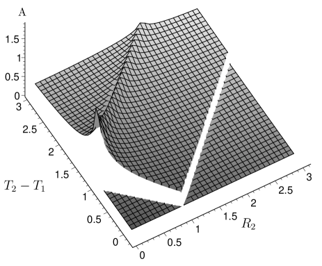
Figure 3: Absolute value $A$ of the commutator of the scalar field $[\hat{\psi}(R_{1},T_{1}),\hat{\psi}(R_{2},T_{2})]$ for $R_{1}=1$ as a function of $T_{2}-T_{1}$ and $R_{2}$. The light cone structure and the singularity at $T_{2}-T_{1}=R_{2}+R_{1}$ can be readily seen. The plot for negative values of $T_{2}-T_{1}$ is obtained by reflecting with respect to the $R_{2}$ axis.

Some interesting properties can be read off from the previous expressions. First of all we see that the commutator is in fact identically zero in the region labeled I; outside it differs from zero. Second we see that it is singular in the line $T_{2}-T_{1}=R_{2}+R_{1}$. It is easy to check that the singularity is logarithmic by using the explicit form of the propagator (17) and expanding around $T_{2}-T_{1}=R_{2}+R_{1}$. This singularity can be understood as a consequence of the presence of the symmetry axis; this is supported by the fact that the $H_{0}$-commutation function satisfies

$$\left(\!\partial_{T}^{2}-\frac{1}{R}\partial_{R}(R\partial_{R})\!\right)\!\cdot[\hat{\psi}(R,T),\hat{\psi}(R_{2},T_{2})]=0\,,$$

$$\left(\!\partial_{T}^{2}-\frac{1}{R}\partial_{R}(R\partial_{R})\!\right)\!\cdot\theta(T-T_{2})[\hat{\psi}(R,T),\hat{\psi}(R_{2},T_{2})]=$$

$$\hskip 85.35826pt\frac{i}{R_{2}}\delta^{(2)}\!(R-R_{2},T-T_{2})\,,$$

which shows that the full commutator is an axially symmetric solution to the 2+1 dimensional wave equation and the future part of it (obtained by multiplying by a step function) is an axially symmetric Green function for the same equation. It is important to point out that even though there is a Minkowskian background metric, the presence of a center of symmetry breaks Lorentz invariance; in fact, the only symmetries of the 2+1 axially symmetric wave equation

$$\left(\!\partial_{T}^{2}-\frac{1}{R}\partial_{R}(R\partial_{R})\!\right)\Phi(T,R)=0$$

that transform solutions $\Phi(T,R)$ into solutions are

i) Translations

$$\Phi(T,R)\mapsto\Phi(T-\epsilon,R)\quad(\epsilon\in\mathbb{R}),$$

ii) Dilatations

$$\Phi(T,R)\mapsto\Phi(e^{\epsilon}T,e^{\epsilon}R)\quad(\epsilon\in\mathbb{R}),$$

iii) Inversions

$$\Phi(T,R)\!\mapsto\frac{\Phi[\tau_{\epsilon}(T,\!R),\rho_{\epsilon}(T,\!R)]}{\sqrt{1\!-\!2T\epsilon\!+\!(T^{2}\!-\!R^{2})\epsilon^{2}}}\!\quad(\epsilon\textrm{ small enough})$$

with

$$\tau_{\epsilon}(T,R) = \frac{T-\epsilon(T^{2}-R^{2})}{1-2T\epsilon+(T^{2}-R^{2})\epsilon^{2}}\,,$$

$$\rho_{\epsilon}(T,R) = \frac{R}{1-2T\epsilon+(T^{2}-R^{2})\epsilon^{2}}\,.$$

These can be obtained systematically by using the general theory of symmetry groups for partial differential equations (see Olver (1993)).

IV.2 $E(H_{0})$ Hamiltonian

Let us consider now the commutator of the field operators obtained in the Heisenberg picture with the quantum Hamiltonian $\hat{H}:=E(\hat{H}_{0})=(1-e^{-4\bar{G}\hat{H}_{0}})/(4G_{3})$. Here $\bar{G}=G_{3}\hbar$, and we have restored the values of the Planck constant and the three-dimensional gravitational constant (but kept $c=1$) to have the possibility of discussing the semiclassical limit. Recall that the Hamiltonian $\hat{H}_{0}$ is given by Eq. (13), where we choose the normalization of the creation and annihilation operators so that the commutation relation (11) is satisfied (with no $\hbar$ in the r.h.s.). Notice that, with this convention, $\hat{A}(k)$, $\hat{H}_{0}$, and $\hat{H}$ have formally the same dimensions as $\bar{G}^{1/2}$ (or $k^{-1/2}$), $k$, and $G_{3}^{-1}$ (or $\hbar k$), respectively. To distinguish the field operators evolved with the new Hamiltonian $\hat{H}$, we will denote them by $\hat{\psi}_{E}(R,t)$. In order to compute the commutator $[\hat{\psi}_{E}(R_{1},t_{1}),\hat{\psi}_{E}(R_{2},t_{2})]$, we make use of the expressions (15) for the creation and annihilation operators evolved in $t$, which can also be written as

$$\hat{A}_{E}(k,t)\! = \!\hat{A}(k)\exp\left[it\left(E(\hat{H}_{0}-k)-E(\hat{H}_{0})\right)\right],$$

$$\hat{A}^{\dagger}_{E}(k,t)\! = \!\hat{A}^{\dagger}(k)\exp\left[it\left(E(\hat{H}_{0}+k)-E(\hat{H}_{0})\right)\right].\hskip 25.6073pt$$ (18)

Substituting then the relation

$$\hat{\psi}_{E}(R,t)=\sqrt{4\bar{G}}\int_{0}^{\infty}\!\!\!dk\,J_{0}(Rk)\left[\hat{A}_{E}(k,t)+\hat{A}_{E}^{\dagger}(k,t)\right],$$

we get the relevant field commutator

$$\big{[}\hat{\psi}_{E}(R_{1},t_{1}),\hat{\psi}_{E}(R_{2},t_{2})\big{]}\!\!=\!\!\!\int_{0}^{\infty}\!\!\!\!\!\!\!dk_{1}\!\!\int_{0}^{\infty}\!\!\!\!\!\!\!dk_{2}J_{0}(R_{1}k_{1})J_{0}(R_{2}k_{2})$$

$$\times 4\bar{G}\bigg{\{}\!\big{[}\hat{A}_{E}(k_{1},\!t_{1}),\hat{A}_{E}(k_{2},\!t_{2})\big{]}\!+\!\big{[}\hat{A}^{\dagger}_{E}(k_{1},\!t_{1}),\hat{A}^{\dagger}_{E}(k_{2},\!t_{2})\big{]}$$

$$+\big{[}\hat{A}_{E}(k_{1},\!t_{1}),\hat{A}^{\dagger}_{E}(k_{2},\!t_{2})\big{]}\!+\!\big{[}\hat{A}^{\dagger}_{E}(k_{1},\!t_{1}),\hat{A}_{E}(k_{2},\!t_{2})\big{]}\bigg{\}}.$$

The commutators involving $\hat{A}_{E}(k,t)$ and $\hat{A}^{\dagger}_{E}(k,t)$ can be found in Appendix A. Note that, in contrast with the evolution given by $H_{0}$, for which the commutation function is a c-number, the situation now is more complicated because $\big{[}\hat{\psi}_{E}(R_{1},t_{1}),\hat{\psi}_{E}(R_{2},t_{2})\big{]}$ is an operator, as it happens in interacting theories. We will analyze two types of matrix elements for it, namely, the expectation value on the vacuum and on one-particle states. In addition, we will briefly comment on the expectation value on coherent states.

$\bullet$ Vacuum expectation value.

$$\langle 0|\,[\hat{\psi}_{E}(R_{1},t_{1}),\hat{\psi}_{E}(R_{2},t_{2})]\,|0\rangle=\hskip 93.89418pt$$

$$i8\bar{G}\!\!\int_{0}^{\infty}\!\!\!\!\!\!dk\,J_{0}(R_{1}k)J_{0}(R_{2}k)\sin\left[\frac{t_{2}-t_{1}}{4\bar{G}}(1\!-\!e^{-4\bar{G}k})\right]\!.\hskip 11.38092pt$$ (19)

In the following we will discuss the differences and similarities of this matrix element and the $H_{0}$-commutation function.

Figure 4: Comparison between the absolute values (over $8\bar{G}$) of the $H_{0}$-commutator and the vacuum expectation value of the $E(H_{0})$-commutator for two different values of $\bar{G}$, plotted for $R_{1}=1$.

We point out that the factor $\sin[(T_{2}-T_{1})k]$ that appears in the integrand of the $H_{0}$-commutator is substituted now by $\sin[(t_{2}-t_{1})(1-e^{-4\bar{G}k})/(4\bar{G})]$. They coincide for $k\rightarrow 0$, but the former of these functions oscillates for all values of $k$ whereas the latter approaches a constant value when $k\rightarrow\infty$. This changes the convergence properties of the integral. In particular it is straightforward to see that the integral (19) diverges whenever $R_{1}=R_{2}$ (except if $\sin\left[(t_{2}-t_{1})/(4\bar{G})\right]=0$) but converges otherwise. Therefore, the vacuum expectation value has a singularity structure that differs from the one given by Eq. (16). This has some interesting physical consequences. First we see that the singularity that originates in the axis in the $H_{0}$ case is not present when the evolution is dictated by $E(H_{0})$; this can be interpreted as a blurring of the axis due to quantum corrections. Second we see that a completely different kind of singularity pops up when the evolution is generated by $E(H_{0})$. From a mathematical point of view its origin is clearly related to the fact that the energy is bounded from above and, hence, for large values of $k$ the integrand is just a product of two $J_{0}$ Bessel functions (which give a divergent integral if their arguments coincide). Physically, the emergence of the singularity can be understood in an intuitive manner by writing a state as a superposition of vectors of the form $\hat{A}^{\dagger}(k)|0\rangle$,

$$\hat{\psi}_{E}(R_{1},t_{1})|0\rangle\!=\!\sqrt{4\bar{G}}\!\int_{0}^{\infty}\!\!\!\!\!\!dk\,J_{0}(R_{1}k)\,e^{\frac{it_{1}}{4\bar{G}}(1-e^{-4\bar{G}k})}\hat{A}^{\dagger}(k)|0\rangle,$$

and projecting onto $\hat{\psi}_{E}(R_{2},t_{2})|0\rangle$. The $e^{it_{j}(1-e^{-4\bar{G}k})/(4\bar{G})}$ factor (for $j=1$ or 2) goes to a phase that depends only on $t_{j}$ as $k\rightarrow\infty$. So, if $R_{1}=R_{2}$, the coefficients of the linear superposition defining, respectively, $\hat{\psi}_{E}(R,t_{1})|0\rangle$ and $\hat{\psi}_{E}(R,t_{2})|0\rangle$ differ only by a constant phase for large values of $k$. This means that, in the sector of large $k$, these two states have coherent phases and therefore a constructive interference. Since each of them has an infinite norm, their scalar product diverges. A similar effect can be found in the quantum dynamics of a free particle with an energy given by a function $E(k)$ with $dE(k)/dk\rightarrow 0$ as $k\rightarrow\infty$. If one builds a wave packet as

$$\Phi(t,x)=\int_{0}^{\infty}dk\,C(k)e^{-i[tE(k)+kx]},$$

with $C(k)$ peaked around a large value of $k$, $k_{0}\gg 1$, the group velocity becomes almost zero and $\Phi(t,x)$ stays essentially the same at every $x$ for long periods of time.

The integral in Eq. (19) can be written explicitly as a convergent series (when $R_{1}\neq R_{2}$) by expanding the sine function as a power series of $e^{-4\bar{G}k}$ and computing the resulting integrals involving two Bessel functions and an exponential Gradshteyn and Ryzhik (1994)

$$\langle 0|\,[\hat{\psi}_{E}(R_{1},t_{1}),\hat{\psi}_{E}(R_{2},t_{2})]\,|0\rangle=\hskip 93.89418pt$$

$$\frac{i8\bar{G}}{\pi\sqrt{R_{1}R_{2}}}\left\{\!\sin(\Delta t)\!\!\sum_{n=0}^{\infty}\!\frac{\!(-1)^{n}(\Delta t)^{2n}\!\!}{(2n)!}Q_{-1/2}\left[\sigma_{2n}(R_{1},R_{2})\right]\right.$$

$$-\left.\!\cos(\Delta t)\!\sum_{n=0}^{\infty}\!\frac{\!(-1)^{n}(\Delta t)^{2n+1}\!\!\!}{(2n+1)!}Q_{-1/2}\!\left[\sigma_{2n+1}(R_{1},R_{2})\right]\!\right\}\!.\hskip 8.5359pt$$ (20)

Here, we have introduced the notation

$$\Delta t=\frac{t_{2}-t_{1}}{4\bar{G}},\hskip 14.22636pt\sigma_{n}(R_{1},R_{2})=\frac{16\bar{G}^{2}n^{2}+R_{1}^{2}+R_{2}^{2}}{2R_{1}R_{2}}.$$

Besides, $Q_{-1/2}(x)=\pi F\left(\frac{3}{4},\frac{1}{4};1;\frac{1}{x^{2}}\right)/\sqrt{2x}$ [with $x>1$] is the associated Legendre function of the second kind Gradshteyn and Ryzhik (1994). We recall that the function $Q_{-1/2}(x)$ grows without bound as the argument approaches $x=1$ and falls off to zero as $\pi/\sqrt{2x}$ when $x\rightarrow\infty$. When $R_{1}=R_{2}$ the singularity in Eq. (LABEL:s2-006) comes just from the $n=0$ term in the first series of the expansion, that is given by

$$\frac{i8\bar{G}}{\pi\sqrt{R_{1}R_{2}}}\,Q_{-1/2}\left(\frac{R_{1}^{2}+R_{2}^{2}}{2R_{1}R_{2}}\right)\sin\left(\frac{t_{2}-t_{1}}{4\bar{G}}\right).$$

A series of plots of $[\hat{\psi}(R_{1},T_{1}=t_{1}),\hat{\psi}(R_{2},T_{2}=t_{2})]$ and $\langle 0|\,[\hat{\psi}_{E}(R_{1},t_{1}),\hat{\psi}_{E}(R_{2},t_{2})]\,|0\rangle$ (both over $8\bar{G}$) is shown in Fig. 4 for fixed values of $R_{1}$ and $t_{2}-t_{1}$ as a function of $R_{2}$, with several choices for $\bar{G}$. We choose $t_{2}-t_{1}$ small enough to guarantee the rapid convergence of the series in Eq. (LABEL:s2-006) and leave a discussion of the behavior of the integral (19) when $\bar{G}\rightarrow 0$ for future work. As we can see $\langle 0|\,[\hat{\psi}_{E}(R_{1},t_{1}),\hat{\psi}_{E}(R_{2},t_{2})]\,|0\rangle$ seems to approach $[\hat{\psi}(R_{1},T_{1}=t_{1}),\hat{\psi}(R_{2},T_{2}=t_{2})]$ at least in a certain average sense when $\bar{G}$ is sufficiently small (though not vanishing). It falls off to zero quite quickly outside the light cone defined by the free commutator and the auxiliary Minkowski metric, and displays an oscillatory behavior within this light cone. The characteristic length of this oscillation decreases with $\bar{G}$, as well as close to the $R_{1}=R_{2}$ singularity. The approximation obtained by truncating the series expansion (LABEL:s2-006), keeping a sufficiently large number of terms, compares well with the results of numerically computing expression (19), at least for low enough values of $t_{2}-t_{1}$.

$\bullet$ Expectation value on one-particle states.

We consider now states of the form

$$|\rho\rangle=\int_{0}^{\infty}\!\!\!\!dk\,f(k)A^{\dagger}(k)|0\rangle$$

where the function $f=|f|e^{i\phi_{f}}$ satisfies $\int_{0}^{\infty}\!dk|f(k)|^{2}=1$. We then have

$$\langle\rho|[\hat{\psi}_{E}(R_{1},t_{1}),\hat{\psi}_{E}(R_{2},t_{2})]|\rho\rangle=$$

$$-i8\bar{G}\!\int_{0}^{\infty}\!\!\!\!\!\!dk_{1}\!\!\int_{0}^{\infty}\!\!\!\!\!\!dk_{2}J_{0}(R_{1}k_{1})\bigg{\{}2J_{0}(R_{2}k_{2})|f(k_{1})f(k_{2})|$$

$$\times\sin{\left[2\bar{G}(t_{1}-t_{2})E(k_{1})E(k_{2})\right]}\cos{\left[\Omega_{f}(k_{1},k_{2})\right]}$$

$$-J_{0}(R_{2}k_{1})|f(k_{2})|^{2}\sin{\left[(t_{2}-t_{1})E(k_{1})e^{-4\bar{G}k_{2}}\right]}\bigg{\}},\hskip 25.6073pt$$ (21)

where

$$\Omega_{f}(k_{1},k_{2}) = 2\bar{G}(t_{2}-t_{1})E(k_{1})E(k_{2})+t_{1}E(k_{1})$$

$$- t_{2}E(k_{2})-\phi_{f}(k_{1})+\phi_{f}(k_{2}).\hskip 11.38092pt$$

A complete discussion of the meaning of the previous expression is beyond the scope of this paper. Nevertheless, some features already present in the vacuum expectation value are also present here; in particular the $R_{1}=R_{2}$ singularity. This can be seen by considering the last term in Eq. (21): the integral in $k_{2}$ is

$$\int_{0}^{\infty}\!\!\!dk_{2}|f(k_{2})|^{2}\sin{\left[(t_{2}-t_{1})E(k_{1})e^{-4\bar{G}k_{2}}\right]},$$

which takes in general a non-vanishing constant value (depending on $t_{2}-t_{1}$ and $\bar{G}$) as $k_{1}\rightarrow\infty$, thus rendering the remaining integral in $k_{1}$ divergent. As the first term in Eq. (21) leads to a convergent integral, we conclude that the expectation value is singular when $R_{1}=R_{2}$.

It is not difficult to obtain as well an explicit expression for the expectation value of the $E(H_{0})$-commutator on the coherent states of the field $\psi$. These diagonal matrix elements are calculated in Appendix B. For our discussion in this work, let us only comment that the result is actually divergent when $R_{1}=R_{2}$. This supplies further support to the claim that the considered singularity is indeed a generic feature of the system.

V Conclusions and perspectives

Linearly polarized cylindrical waves can be studied in great detail both from the classical and quantum points of view. As we have seen, there are two relevant Hamiltonians for the study of the system. We have shown that the action and the metric of the gauge-fixed model in linearized gravity reproduce the results obtained by considering full cylindrical gravity and working to the first perturbative order. We get in this way a free Hamiltonian. The Hamiltonian governing the dynamics of the full system, on the other hand, is different from the free one, but turns out to be a function of it and presents certain features with deep physical consequences, like e.g. the existence of an upper bound.

We have studied the similarities and differences of these two admissible kinds of evolution; in particular, we have discussed how the emergence of an upper bound for the energy affects the causal structure of the model and the spreading of the light cones. The field commutator for the free Hamiltonian is a c-number and shows the typical light cone structure found in standard perturbative quantum field theories. The commutator for the physical Hamiltonian, as it usually happens for interacting theories, is no longer a c-number, so one has to consider its matrix elements. By concentrating on the vacuum expectation value we have been able to see several interesting phenomena: a spreading of the light cone as a function of the gravitational constant, the disappearance of the singularity present in the free case due to the smearing of the symmetry axis and the appearance of a new type of singularity associated with the fact that the energy is bounded from above. This new singularity is also present in the other expectation values discussed in the paper, namely for one-particle states and coherent states, and appears to be a generic feature of the model.

There are several open questions that we plan to address in future work. In particular, it would be desirable to reach a better understanding of the behavior of the field commutator in the limit in which the length scale provided by $\bar{G}$ goes to zero. The expectation values of the $E(H_{0})$-commutator discussed here resemble those derived from the free Hamiltonian $H_{0}$ at least in a certain average sense. However it is not obvious how precisely and up to what extent they actually relate to each other. This is partly so because of the different singularity structure found in both cases. Further research on this subject will concentrate on the properties of the model in the semiclassical limit $\bar{G}\rightarrow 0$. We will also pay detailed attention to matrix elements of the field commutator other than the vacuum expectation value, with the aim at discussing how the smearing of the light cones depends on the energy.

Appendix A Useful Commutators

In this appendix, we compute the commutators of the creation and annihilation operators $\hat{A}_{E}(k,t)$ and $\hat{A}^{\dagger}_{E}(k,t)$, obtained from the corresponding operators $\hat{A}(k)$ and $\hat{A}^{\dagger}(k)$ via the unitary evolution generated by $E(\hat{H}_{0})$, where $\hat{H}_{0}=\int^{\infty}_{0}dkk\hat{A}^{\dagger}(k)\hat{A}(k)$. Employing relations (18) and the basic commutators (11), it is possible to show that

$$\bullet\,\big{[}\hat{A}_{E}(k_{1},t_{1}),\hat{A}_{E}(k_{2},t_{2})\big{]} = \hat{A}(k_{1})\hat{A}(k_{2})\exp\left[it_{1}E(\hat{H}_{0}-k_{1}-k_{2})+i(t_{2}-t_{1})E(\hat{H}_{0}-k_{2})-it_{2}E(\hat{H}_{0})\right]$$

$$- \hat{A}(k_{1})\hat{A}(k_{2})\exp\left[it_{2}E(\hat{H}_{0}-k_{1}-k_{2})+i(t_{1}-t_{2})E(\hat{H}_{0}-k_{1})-it_{1}E(\hat{H}_{0})\right]\,,$$

$$\bullet\,\big{[}\hat{A}^{\dagger}_{E}(k_{1},t_{1}),\hat{A}^{\dagger}_{E}(k_{2},t_{2})\big{]} = \hat{A}^{\dagger}(k_{1})\hat{A}^{\dagger}(k_{2})\exp\left[it_{1}E(\hat{H}_{0}+k_{1}+k_{2})+i(t_{2}-t_{1})E(\hat{H}_{0}+k_{2})-it_{2}E(\hat{H}_{0})\right]$$

$$- \hat{A}^{\dagger}(k_{1})\hat{A}^{\dagger}(k_{2})\exp\left[it_{2}E(\hat{H}_{0}+k_{1}+k_{2})+i(t_{1}-t_{2})E(\hat{H}_{0}+k_{1})-it_{1}E(\hat{H}_{0})\right]\,,$$

$$\bullet\,\big{[}\hat{A}_{E}(k_{1},t_{1}),\hat{A}^{\dagger}_{E}(k_{2},t_{2})\big{]} = \hat{A}(k_{1})\hat{A}^{\dagger}(k_{2})\exp\left[it_{1}E(\hat{H}_{0}+k_{2}-k_{1})+i(t_{2}-t_{1})E(\hat{H}_{0}+k_{2})-it_{2}E(\hat{H}_{0})\right]$$

$$- \hat{A}^{\dagger}(k_{2})\hat{A}(k_{1})\exp\left[it_{2}E(\hat{H}_{0}+k_{2}-k_{1})+i(t_{1}-t_{2})E(\hat{H}_{0}-k_{1})-it_{1}E(\hat{H}_{0})\right]\,,$$

$$\bullet\,\big{[}\hat{A}^{\dagger}_{E}(k_{1},t_{1}),A_{E}(k_{2},t_{2})\big{]} = \hat{A}^{\dagger}(k_{1})\hat{A}(k_{2})\exp\left[it_{1}E(\hat{H}_{0}+k_{1}-k_{2})+i(t_{2}-t_{1})E(\hat{H}_{0}-k_{2})-it_{2}E(\hat{H}_{0})\right]$$

$$- \hat{A}(k_{2})\hat{A}^{\dagger}(k_{1})\exp\left[it_{2}E(\hat{H}_{0}+k_{1}-k_{2})+i(t_{1}-t_{2})E(\hat{H}_{0}+k_{1})-it_{1}E(\hat{H}_{0})\right].$$

Appendix B Expectation values on coherent states

We consider coherent states of the field $\psi$, given by

$$|\Psi_{C}\rangle = K_{C}\exp{\left(\int_{0}^{\infty}\!\!\!\frac{dk}{\sqrt{8\bar{G}}}\,C(k)A^{\dagger}(k)\right)}|0\rangle$$

$$= K_{C}\sum_{n=0}^{\infty}\frac{1}{n!}\left(\int_{0}^{\infty}\!\!\!\frac{dk}{\sqrt{8\bar{G}}}\,C(k)A^{\dagger}(k)\right)^{n}|0\rangle,$$

where $C(k)$ is a square integrable function and $K_{C}$ is a normalization constant satisfying

$$|K_{C}|^{2}=\exp\left(-\int_{0}^{\infty}\!\frac{dk}{8\bar{G}}\,|C(k)|^{2}\right).$$

The expectation value of the $E(H_{0})$-commutator is

$$\langle\Psi_{C}|\big{[}\hat{\psi}_{E}(R_{1},t_{1}),\hat{\psi}_{E}(R_{2},t_{2})\big{]}|\Psi_{C}\rangle=\hskip 68.28644pt$$

$$\int_{0}^{\infty}\!\frac{dk_{1}}{2}\!\!\int_{0}^{\infty}\!\!\!\!\!\!dk_{2}J_{0}(R_{1}k_{1})J_{0}(R_{2}k_{2})\sum_{s=0}^{\infty}\frac{I_{s}(C)}{s!}G_{s}(k_{1},k_{2}),$$

where

$$I_{s}(C)=\exp\left\{\int_{0}^{\infty}\!\frac{dk}{8\bar{G}}\,|C(k)|^{2}\left(e^{-4\bar{G}sk}\!-\!1\right)\right\},\hskip 34.14322pt$$

$$G_{s}(k_{1},k_{2})=8\bar{G}\delta(k_{1},k_{2})\bigg{\{}[b(k_{1},-k_{2})]^{s}\!\!-\![b(k_{2},-k_{1})]^{s}\!\bigg{\}}$$

$$+\overline{C}(k_{2})C(k_{1})\bigg{\{}[b(k_{1},-k_{2})]^{s}\!-\![b(-k_{2},k_{1})]^{s}\bigg{\}}e^{-4\bar{G}sk_{1}}\hskip 5.69046pt$$

$$+\overline{C}(k_{1})C(k_{2})\bigg{\{}[b(-k_{1},k_{2})]^{s}\!-\![b(k_{2},-k_{1})]^{s}\bigg{\}}e^{-4\bar{G}sk_{2}}\hskip 5.69046pt$$

$$+C(k_{1})C(k_{2})\bigg{\{}[b(k_{1},k_{2})]^{s}\!-\![b(k_{2},k_{1})]^{s}\bigg{\}}e^{-4\bar{G}s(k_{1}+k_{2})}$$

$$+\overline{C}(k_{1})\overline{C}(k_{2})\bigg{\{}[b(-k_{1},-k_{2})]^{s}\!-\![b(-k_{2},-k_{1})]^{s}\bigg{\}},\hskip 19.91684pt$$

and we have employed the notation

$$b(k_{n},k_{m}) = \!\frac{-i}{4\bar{G}}\left[t_{n}e^{4\bar{G}k_{m}}(e^{4\bar{G}k_{n}}\!-\!1)+t_{m}(e^{4\bar{G}k_{m}}\!-\!1)\right].$$

Note that, when $R_{1}=R_{2}$, the delta in the expression of $G_{s}(k_{1},k_{2})$ leads to the divergent integral

$$\int_{0}^{\infty}\!\!\!\!\!dk\,J_{0}^{2}(R_{1}k)\!\sum_{s=0}^{\infty}\frac{8\bar{G}I_{2s+1}}{(2s+1)!}\left[\frac{i(t_{2}-t_{1})(1-e^{-4\bar{G}k})}{4\bar{G}}\right]^{\!2s+1}\!\!\!\!\!\!\!\!.$$

References

• Ashtekar (1996) A. Ashtekar, Phys. Rev. Lett. 77, 4864 (1996).
• Ashtekar and Pierri (1996) A. Ashtekar and M. Pierri, J. Math. Phys. 37, 6250 (1996).
• Angulo and Mena Marugan (2000) M. E. Angulo and G. A. Mena Marugán, Int. J. Mod. Phys. D 9, 669 (2000).
• Gambini and Pullin (1997) R. Gambini and J. Pullin, Mod. Phys. Lett. A 12, 2407 (1997).
• Dominguez and Tiglio (1999) A. E. Domínguez and M. H. Tiglio, Phys. Rev. D 60, 064001 (1999).
• Varadarajan (2000) M. Varadarajan, Class. Quant. Grav. 17, 189 (2000).
• Cruz, Miković and Navarro-Salas (1998) J. Cruz, A. Miković and J. Navarro-Salas, Phys. Lett. B 437, 273 (1998).
• Romano and Torre (1996) J. D. Romano and C. G. Torre, Phys. Rev. D 53, 5634 (1996).
• Korotkin (1998) D. Korotkin and H. Samtleben, Phys. Rev. Lett. 80, 14 (1998).
• Kuchař (1971) K. Kuchař, Phys. Rev. D 4, 955 (1971).
• Ashtekar, Bičák and Schmidt (1997) A. Ashtekar, J. Bičák and B. G. Schmidt, Phys. Rev. D 55, 669 (1997); eprint ibid 687 (1997).
• Peskin (1995) M. E. Peskin and D. V. Schroeder, An Introduction to quantum field theory (Addison-Wesley, Reading, USA, 1995).
• Pauli (1940) W. Pauli, Phys. Rev. 58, 716 (1940).
• Ashtekar and Varadarajan (1994) A. Ashtekar and M. Varadarajan, Phys. Rev. D 50, 4944 (1994).
• Varadarajan (1995) M. Varadarajan, Phys. Rev. D 52, 2020 (1995).
• Leoński (1998) W. Leoński, Acta Phys. Slovaca 48, 371 (1998); J. Banerji, Pramana J. Phys. 56, 267 (2001).
• Einstein and Rosen (1937) A. Einstein and N. Rosen, J. Franklin Inst. 223, 43 (1937).
• Melvin (1965) K. S. Thorne, Phys. Rev. 138, B251 (1965); M. A. Melvin, Phys. Rev. 139, B225 (1965).
• Reed and Simon (1975) M. Reed and B. Simon, Methods of Modern Mathematical Physics II: Fourier Analysis, Self Adjointness (Academic Press, Cambridge, England, 1975).
• Allen (1987) M. Allen, Class. Quantum Grav. 4, 149 (1987).
• Gradshteyn and Ryzhik (1994) I. S. Gradshteyn and I. M. Ryzhik, Table of Integrals, Series and Products, 5th ed. (Academic Press, London, 1994).
• Olver (1993) P. J. Olver, Aplications of Lie Groups to Differential Equations, 2nd ed. (Springer-Verlag, New York, 1993).