GWDAW 2002

Abstract

In this work we estimate the performance of a method for the detection of burst events in the data produced by interferometric gravitational wave detectors. We compute the receiver operating characteristics in the specific case of a simulated noise having the spectral density expected for Virgo, using test signals taken from a library of possible waveforms emitted during the collapse of the core of Type II Supernovae.

1 Introduction

Several large scale interferometric instruments are being commissioned [1, 2] or have started science runs [3, 4], aiming at the detection of gravitational waves (GW) emitted by astrophysical sources. The interferometers are sensible in a relatively wide frequency band, which makes it possible to resolve the structure of short bursts of GW, like those emitted during the Type II supernova explosions, or the merger phase in the binary black-holes coalescence (see [5] and references therein).

However it has been frequently argued [6, 7] that the knowledge of the burst waveforms is rather poor, and therefore the classical Wiener filtering may be not applicable: in this context, it is advisable to develop methods which do not rely on the theoretical signal waveform (see [8] for a recent review). One of us (A.V.) has proposed in [9] one such method, which is claimed to be “optimal” under the assumptions that only the duration of the burst is known, and that the detector noise is Gaussian, but not necessarily white.

In [9] the method has been derived from those assumptions, and an algorithm has been defined that we will call “generalized delta filtering” (GDF), because it reduces itself to a $\delta$-filtering when its “window size” parameter is chosen to be $1$. In that paper no test was made to assess the actual detection performance of the GDF.

In the present work we have made such a test, using simulated waveforms [10] and the expected Virgo spectral noise density [12].

2 The method in brief

Referring to [9] for details about the method and its derivation, we just recall that in the single detector case it amounts to apply a few simple analysis steps:

1. a $\delta$-filtering step, also called double whitening [11], which can be implemented in the frequency domain dividing the Fourier transform (FT) of the signal by the estimated spectral noise density;

2. estimate the Discrete Karhounen-Loève basis for a window of fixed size $N$ of the $\delta$-filtered data; we recall that the DKL basis is a set of $N$ vectors which “diagonalize” the input noise, in the sense that coefficients $c_{k}\equiv\mathbf{x}\cdot{\bm{\psi}}_{k}$ of the decomposition of data $\mathbf{x}$ over the basis are statistically independent, that is $E\left[c_{k}c_{l}\right]\propto\delta_{kl}$ [13];

3. slide the window over the available $\delta$-filtered data and compute the statistic

   $$L=\sum_{k=1}^{N}\frac{1}{\sigma_{k}}\left({\bm{\psi}}_{k}\cdot\mathbf{x}\right)^{2}$$ (1)

   where $\sigma_{k}$ and ${\bm{\psi}}_{k}$ are the eigenvalues and eigenvectors of the DKL basis;

4. select candidates by comparing the data against a threshold $\eta$.

The only parameter of the algorithm is the window size $N$, and possibly the stride used in sliding the window over the $\delta$-filtered data.

3 The simulation

3.1 Input noise

We have used “standard” Virgo noise [12], as modeled on the basis of the expected noise sources [14], including the thermal and shot noise in the frequency band $[10,\,10000]$Hz.

To generate noisy data, we started from white Gaussian noise, “colored” on the basis of the Virgo sensitivity curve.

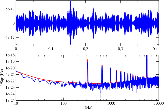
Figure 1: In the lower part, the expected spectral noise density of the Virgo detector is shown, superimposed to an example of spectrum obtained on simulated data. In the upper part, an example of noisy output is plotted in the time domain.

We show in Figure 1 an example of the simulated noise obtained using this procedure. Also the resulting spectrum is shown, superimposed to the “theoretical” spectrum. It is worth noting that the simulated data include the effect of the narrow resonances corresponding to the suspension “violin modes”: it is yet not completely clear if these resonances will be filtered out before applying the detection algorithms, and we have chosen not to remove them.

3.2 Simulated signals

As prototype GW signals, we have used waveforms resulting from simulations of the core-collapse of Type II supernovae made by Zwerger and Müller [10]. These waveforms are labeled by the values of the parameters $A,B,G$ which enter in the polytropic equation of state of the nuclear matter.

Our method is not optimal in the Wiener sense, and therefore it is crucial to set the scale of the signals in the simulations. We have chosen to normalize all the signals to the same intrinsic signal to noise ratio, defined as usual by:

$$\textrm{SNR}_{\textrm{intrinsic}}\equiv\sqrt{4\int_{0}^{\infty}\frac{\left|\tilde{s}\left(f\right)\right|^{2}}{S_{n}\left(f\right)}df}$$ (2)

where $S_{n}$ is the one-sided spectral density of the noise, and $\tilde{s}$ is the FT of the signal considered.

In our simulations we have set $\textrm{SNR}_{\textrm{intrinsic}}=5$ to compare with the results in [8].

3.3 Examples of filtering chain

It is instructive to have a first exploratory look at the results of a GDF analysis performed as in Section 2.

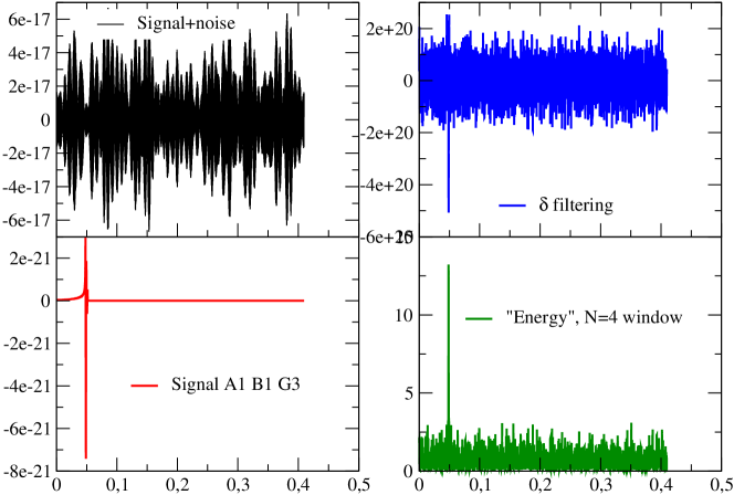
Figure 2: In anti-clockwise sense: simulated signal+noise, signal only, output of a $\delta$-filtering step, output of a GDF analysis using an $N=4$ window.

In Figure 2 we show what happens with an $N=4$ window, choosing a Zwerger-Müller (ZM) signal with a rather short duration, and very much like an instantaneous burst. In this case, the outputs of both the $\delta$-filtering and the GDF analysis put clearly in evidence the event occurrence.

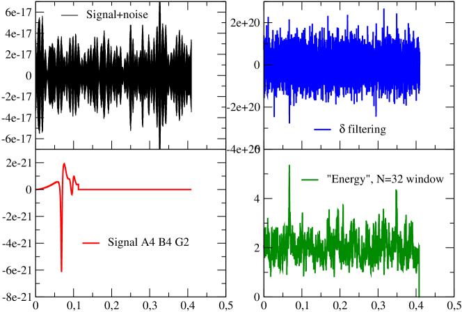
Figure 3: In anti-clockwise sense: simulated signal+noise, signal only, output of a $\delta$-filtering step, output of a GDF analysis using an $N=32$ window.

In Figure 3 we choose a signal having a more complicated time-domain evolution: in this case, the $\delta$-filtering is unable to capture the event, but a GDF analysis using an $N=32$ window appears instead to put it in evidence, although other false alarms appear in the same time window, whose significance remains to be assessed.

These examples are just indications that the method works: for a quantitative understanding we need to estimate the receiver operating characteristics (ROC).

4 The ROC estimation

It is worth recalling that the statistical properties of the GDF detector can be assessed analytically, because the statistic in Equation 1 is just a $\chi^{2}$ with $N$ degrees of freedom.

In presence of a signal, the statistic is a non-central $\chi^{2}$, and its distribution is [9]

$$d\left(L|\textrm{SNR}\right)\textrm{=}\frac{L^{N/2-1}}{s^{N/2}\Gamma\left(\frac{N}{2}\right)}e^{-\frac{1}{2}\left(L+\sqrt{2N}\textrm{SNR}\right)}\,_{0}F_{1}\left(;\frac{N}{2};\frac{\textrm{SNR}\,L\sqrt{2N}}{4}\right)$$ (3)

where ${}_{0}F_{1}$ is the hypergeometric function. The distribution $d\left(L|\textrm{SNR}\right)$ depends only on the SNR of the signal, as seen by the GDF method. Note that this SNR has nothing to do with the $\textrm{SNR}_{\textrm{intrinsic}}$, and it is defined as customary by the ratio

$$\textrm{SNR}\equiv\frac{E\left[L|H_{1}\right]-E\left[L|H_{0}\right]}{\sqrt{E\left[\left(L-E\left[L|H_{0}\right]\right)^{2}|H_{0}\right]}}$$ (4)

where $H_{0}$ and $H_{1}$ are the hypotheses of absence or presence of a signal, respectively. Using this definition it is immediate to show that

$$\textrm{SNR}=\frac{1}{\sqrt{2N}}\sum_{k}\frac{1}{\sigma_{k}}\left({\bm{\psi}}_{k}\cdot\mathbf{x}\right)^{2}$$ (5)

for the GDF statistic.

In order to estimate false alarms and detection probabilities, we need therefore first to compute how much SNR is collected by the GDF detector(s), for a fixed $\textrm{SNR}_{\textrm{intrinsic}}$.

4.1 SNR distribution of the ZM signals

We have considered the 78 signals in the ZM family [10], normalized w.r.t. the theoretical Virgo noise to have $\textrm{SNR}_{\textrm{intrinsic}}=5$, and we have computed for each of them the SNR resulting from a GDF analysis, using different values of the window size $N$. We stress that there is no point in comparing the values of SNR for different detection methods or different window sizes $N$: only the comparison of false alarm and detection probabilities is sensible.

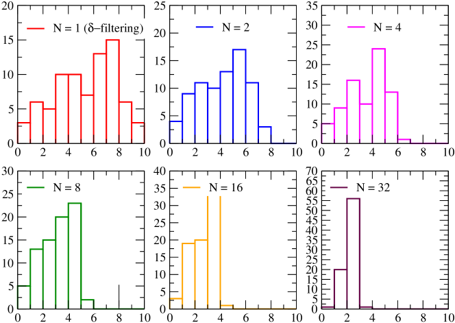
Figure 4: The distribution of SNR for different values of the $N$ parameter of the GDF algorithm, based on ZM input signals normalized to have $\textrm{SNR}_{\textrm{intrinsic}}=5$

We show in Figure 4 the resulting SNR distributions.

4.2 False alarm and detection probabilities

Starting from the distribution in Equation 3 it is immediate to derive the false alarm probability

$$P_{FA}\left(\eta\right)\equiv\int_{\eta}^{\infty}d\left(L|0\right)dL=\frac{\Gamma\left(\frac{\eta}{2};\frac{N}{2}\right)}{\Gamma\left(\frac{N}{2}\right)}$$ (6)

while the detection probability $P_{DET}\left(\eta|\textrm{SNR}\right)$ can be evaluated by a numerical integral.

We stress that these $P_{DET},P_{FA}$ are “per bin”, namely they do not take into account the auto-correlation of the filter outputs, which would require to resample the output or to select, among the outputs above threshold, only the maxima over a fixed time window, whose length would be another parameter of the algorithm.

For a given signal, we have varied the threshold $\eta$ to obtain $P_{DET}$ as a function of $P_{FA}$, and for each value of $\eta$ we have averaged the probabilities over the different ZM waveforms; the resulting plot of $P_{DET}$ against $P_{FA}$ constitutes the average ROC curve, that we show in Figure 5 for different values of $N$.

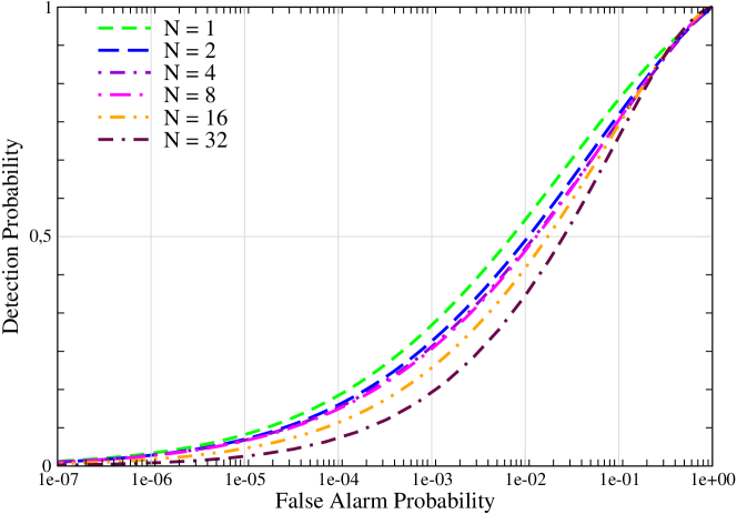
Figure 5: The ROC curves obtained averaging over the 78 waveforms of the ZM family (see text), for different window sizes $N$

The similarity of the plots may lead to argue that the window size is not very important. Actually this is just an effect of the averaging, as indicated by the examples in Figures 2 and 3, which show that one should better match the signal length and the window size $N$.

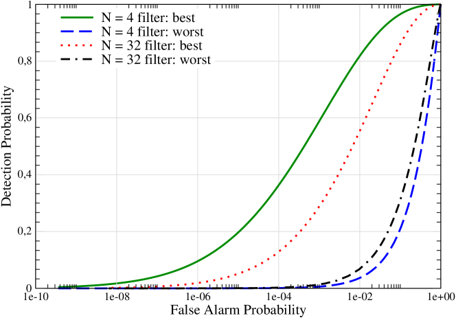
Figure 6: The best and worst cases of the ROC curves, obtained over the different ZM waveforms, for two different values of the $N$ parameter. Note that the horizontal scale is different from the one used in Figure 5

This is confirmed in Figure 6, where we plot the best and worst ROC curve obtained over the 78 ZM signals, for two different values (4 and 32) of the $N$ parameter. The large dispersion of the results is a consequence of the large differences of the SNR recovered by the GDF filters over the various waveforms, as displayed in Figure 4.

5 Conclusions

In this paper we have started to assess the detection capabilities of the “generalized delta filtering” introduced by one of us in [9], by computing the receiver operating characteristics in the case of Virgo simulated noise, using signals from the Zwerger-Müller family.

The ROC curves we obtain are generally inferior to those obtained by some other burst detection methods [8]; however we should mention that in [8] a white Gaussian noise was used, a difference with our computations whose relevance we are unable to assess.

The results show a wide variation over the $N$ parameter, and suggest that further optimization is possible: one should define a bank of filters with different $N$ values and understand how to combine the various outputs and how to select candidates. As discussed in Section 4.2 one should take into account the fact that the filter outputs are correlated, and that one may strongly decrease the false alarm probability by re-sampling the output at a lower rate, while probably not hampering too much the detection probability.

These studies are beyond the scope of the present work and will be the subject of a forthcoming paper.

References

References

- [1] K Danzmann et al., in First Edoardo Amaldi conference on gravitational wave experiments, eds. E Coccia et al., World Scientific, Singapore (1995).
- [2] B Caron et al., Class.Quant.Grav., 14, 1461 (1997).
- [3] A Abramovici et al., Science 256, 325 (1992).
- [4] K Tsubono et al., in First Edoardo Amaldi conference on gravitational wave experiments, eds. E Coccia et al., World Scientific, Singapore (1995).
- [5] N Arnaud, M Davier, F Cavalier and P Hello, Phys.Rev.D 59, 082002 (1999).
- [6] É É Flanagan, S A Hughes, Phys.Rev.D 57, 4566 (1998).
- [7] T Pradier, et al Phys.Rev.D 63, 042002 (2001).
- [8] N Arnaud et al., Comparison of filters for detecting gravitational wave fursts in interferometric detectors, gr-qc/0210098, to appear in Phys.Rev.D
- [9] A Viceré, Phys.Rev.D 66, 062002 (2002).
- [10] T Zwerger and E Müller, Astron.Astrophys. 267, 623 (1993).
-
[11]
E Cuoco,
Wiener filtering and nonstationary noise: detection
efficiency and undetected nonlinearities,
http://amaldi.ligo.caltech.edu:8083/related/talks/22/cuoco.pdf - [12] http://www.virgo.infn.it/senscurve
- [13] C W Therrien, Discrete random signals and statistical signal processing, Prentice-Hall, Englewood Cliffs, (1992).
- [14] M Punturo, The Virgo sensitivity curve, Virgo internal note VIR-NOT-PER-1390-51 (2001).