Gravitational Wave Confusion Noise

Abstract

One of the greatest challenges facing gravitational wave astronomy in the low frequency band is the confusion noise generated by the vast numbers of unresolved galactic and extra galactic binary systems. Estimates of the binary confusion noise suffer from several sources of astrophysical uncertainty, such as the form of the initial mass function and the star formation rate. There is also considerable uncertainty about what defines the confusion limit. Various ad-hoc rules have been proposed, such as the one source per bin rule, and the one source per three bin rule. Here information theoretic methods are used to derive a more realistic estimate for the confusion limit. It is found that the gravitational wave background becomes unresolvable when there is, on average, more than one source per eight frequency bins. This raises the best estimate for the frequency at which galactic binaries become a source of noise from 1.45 mHz to 2.54 mHz.

Population synthesis models and astronomical observations suggest that there may be as many as $2\times 10^{8}$ galactic disk binaries containing two compact objects. Several million of these binaries are expected to emit gravitational waves that can be detected by the Laser Interferometer Space Antenna (LISA). At frequencies below $\sim 1$ mHz these systems constitute an embarrassment of riches for gravitational wave astronomy as the number of sources is so great that it becomes impossible to isolated individual binaries. The unresolved galactic gravitational wave background is a source of noise that degrades LISA’s ability to detect other sources, such as extra-galactic supermassive black hole binaries.

A much quoted definition of the gravitational wave confusion noise level is the amplitude at which there is, on average, at least one source per frequency bin. Even this crude definition takes into account some data analysis considerations as the width of a frequency bin, $\Delta f=1/T$, depends on the observation time $T$. The longer the observation, the smaller the confusion noise. However, Hellings ron pointed out that there was not enough information in one frequency bin to fully specify a binary system. A monochromatic, circular binary is described by the seven parameters $(f,\ln{\cal A},\theta,\phi,\imath,\psi,\varphi_{0})$, where $f$ is the gravitational wave frequency, ${\cal A}$ is the intrinsic amplitude, $(\theta,\phi)$ describe the sky location, $\imath$ denotes the inclination, $\psi$ is the polarization angle and $\varphi_{0}$ is the orbital phase. Hellings reasoned that each frequency bin only contains two pieces of information - the real and imaginary parts of the strain spectral density - while six pieces of information are needed to fix $(\ln{\cal A},\theta,\phi,\imath,\psi,\varphi_{0})$. Thus, at least three frequency bins are required to solve for the six parameters. The frequency was not included in the information budget on the grounds that it came for free from the Fourier transform. While the three bin rule is an improvement over the naive one bin rule, it lacks a rigorous justification. More recently, Phinney sterl has revisited the confusion noise question by using Shannon information theory to estimate the total number of binaries than can be resolved by LISA. Here a similar approach is used to estimate the number of frequency bins that are needed to resolve a binary system.

The estimate is made by comparing the information contained in one frequency bin with the amount of information required to record the parameters that describe a binary system. Both of these quantities depend on the signal to noise ratio of the instrument. A higher signal to noise ratio means more information in each bin, but it also means that the binary parameters are better determined, and thus take more information to describe.

The Baud rate of the detector, $C$, depends on the bandwidth of the signal, $B$, and the signal to noise ratio $S/N$ according to

$$C=B\,{\rm log}_{2}\left(1+\frac{S}{N}\right)\,.$$ (1)

The total number of bits transmitted during an observation time $T$ is simply $CT$. Setting the bandwidth equal to $\Delta f=1/T$, it follows that the amount of information per bin is equal to $\Delta I={\rm log}_{2}\left(1+\frac{S}{N}\right)$. Because the LISA observatory is designed to operate in stereo, i.e. LISA can detect both gravitational wave polarizations curt , the total amount of information available in each frequency bin is larger than $\Delta I$, but not a full factor of two larger as the information in each channel is not fully independent. The analysis of the stereo performance is further complicated by the correlated noise in the two channels. In what follows, the information budget is calculated for a single channel, with the expectation that the result would be little changed by including the second channel.

The amount of information required to record the parameters of a binary system can be estimated by comparing the volume of the error ellipsoid to the volume of the parameter space. To see how this works, consider the following one dimensional example. Suppose that the angle $\phi$ can be measured to an accuracy of three degrees. Recording $\phi$ to this accuracy takes $\log_{2}(360/3)\approx 7$ bits of data. The volume of the seven dimensional error ellipsoid that characterizes the binary subtraction problem for LISA can be estimated by calculating the determinant of the Fisher information matrix $\Gamma_{ij}$. To calculate the Fisher matrix an expression is needed that describes how information about the binary is encoded in the the detector output. At low frequencies, the signal in each LISA channel takes the form

$$s_{(}t) = F^{+}(t,\psi,\theta,\phi)A_{+}({\cal A},\imath)\cos\Psi(t,f,\theta,\phi,\varphi_{0})$$ (2)

$$+F^{\times}(t,\psi,\theta,\phi)A_{\times}({\cal A},\imath)\sin\Psi(t,f,\theta,\phi,\varphi_{0})\,,$$

where

$$\Psi(t,f,\theta,\phi,\varphi_{0})=2\pi ft+\Phi_{D}(t,f,\theta,\phi)+\varphi_{0}\,.$$ (3)

Expressions for the detector response functions $F^{+}$ and $F^{\times}$, the Doppler modulation $\Phi_{D}$, and the gravitational wave amplitudes $A_{+}$ and $A_{\times}$ can be found in Ref. cr1 . The components of the Fisher matrix are found using the expression curt

$$\Gamma_{ij}(\vec{\lambda})=\frac{1}{S_{n}(f)}\int_{0}^{T}\partial_{i}s_{\alpha}(t)\partial_{j}s_{\alpha}(t)\,dt\,,$$ (4)

where the components $i,j$ range over the seven parameters $\vec{\lambda}\rightarrow(f,\ln{\cal A},\theta,\phi,\imath,\psi,\varphi_{0})$, and $S_{n}(f)$ is the one-sided noise spectral density. In general, the Fisher matrix is a complicated function of all seven parameters, which implies that the volume of the error ellipsoid varies depending on where the binary sits in parameter space. Assuming that the noise is Gaussian, and working in the limit where the signal is large compared to the noise, the volume of the seven dimensional error ellipsoid is give by

$$\Delta V(\vec{\lambda})=\frac{\pi^{3}\sqrt{2}}{105}\sqrt{{\rm det}(C_{ij}(\vec{\lambda}))}\,,$$ (5)

where $C_{ij}\simeq\Gamma_{ij}^{-1}$ is the noise covariance matrix, $C_{ij}=\langle\Delta\lambda_{i}\Delta\lambda_{j}\rangle$. The amount of information needed to describe or subtract a binary source emitting gravitational waves with frequency $f$ is given by

$${\cal I}(B,\vec{\lambda})=\log_{2}\left(\frac{V(B)}{\Delta V(\vec{\lambda})}\right)\,,$$ (6)

where $V(B)$ is the volume of the parameter space in a bandwidth $B$. The bandwidth needed to subtract a typical binary can be estimated by solving the transcendental equation

$${\cal I}(B)=BT\log_{2}\left(\frac{S}{N}\right)\,,$$ (7)

for $B$. Here ${\cal I}(B)$ is the average amount of information required to remove one binary, and $S/N\gg 1$ is the average signal to noise ratio across the bandwidth. Note that the left hand side of the transcendental equation depends logarithmically on the bandwidth and the observation time, while the right hand side depends linearly on these quantities.

Calculating ${\cal I}(B,\vec{\lambda})$ is a straightforward, yet computationally intensive task. The volume of the error ellipsoid can be expressed in terms of the eigenvalues $\sigma^{2}_{i}$ of the covariance matrix $C_{ij}$:

$$\Delta V(\vec{\lambda})=\frac{\pi^{3}\sqrt{2}}{105}\prod_{i=1}^{7}\sigma_{i}(\vec{\lambda})\,.$$ (8)

The eigenvectors of the covariance matrix lie along the principle axes of the error ellipsoid, which may not be aligned with the coordinate axes. The Fisher matrix can be expressed in the form

$$\Gamma_{ij}(\vec{\lambda})=\left(\frac{S}{N}\right)^{2}\gamma_{ij}(f,\theta,\phi,\imath,\psi)$$ (9)

where the signal strength is given by

$$S^{2}=\int_{0}^{T}s(t)^{2}\,dt$$ (10)

and

$$\gamma_{ij} = \Bigl{(}\int_{0}^{T}\Bigl{[}\partial_{i}C_{+}\partial_{j}C_{\times}+C_{\times}\left(\partial_{i}C_{+}\partial_{j}\Psi+\partial_{j}C_{+}\partial_{i}\Psi\right)$$

$$\quad+\partial_{j}C_{+}\partial_{i}C_{\times}-C_{+}\left(\partial_{i}C_{\times}\partial_{j}\Psi+\partial_{j}C_{\times}\partial_{i}\Psi\right)$$

$$\quad+\left(C_{+}^{2}+C_{\times}^{2}\right)\partial_{i}\Psi\partial_{j}\Psi\Bigr{]}dt\Bigr{)}/\Bigl{(}\int_{0}^{T}\left(C_{+}^{2}+C_{\times}^{2}\right)dt\Bigr{)}.$$

Here $C_{+}(t)=F^{+}(t)A_{+}$ and $C_{\times}(t)=F^{\times}(t)A_{\times}$. The amplitude modulation functions $C_{+}(t)$ and $C_{\times}(t)$ depend on $(\ln{\cal A},\imath,\psi,\theta,\phi)$ but are independent of $f$ and $\varphi_{0}$, while the phase function $\Psi(t)$ depends on $(f,\theta,\phi,\varphi_{0})$ but is independent of $\ln{\cal A},\imath$ and $\psi$. In other words, the amplitude modulation terms are solely responsible for determining the intrinsic amplitude, inclination and polarization, while the phase term is solely responsible for determining the frequency and orbital phase. Both the amplitude and phase play a role in fixing the sky location $(\theta,\phi)$.

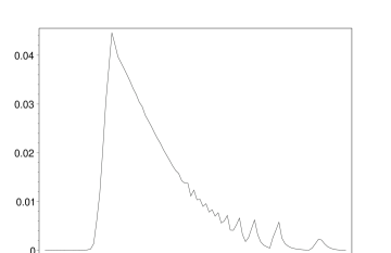
Figure 1: A histogram of the quantity $\log_{10}({\rm vol}(\vec{\lambda}))$.

Using the expressions derived in Ref. cr1 it is a simple, yet laborious task to compute $\gamma_{ij}(f,\theta,\phi,\imath,\psi)$. The final expressions are long and rather opaque. Most striking is the strong dependence on $(f,\theta,\phi,\imath,\psi)$, which makes it exceedingly difficult to give simple answers to questions such as “what is the angular resolution of the LISA detector?”. One trend that is obvious is the improvement in the information encoding at high frequencies that comes from the Doppler modulation. Thus, to obtain a lower limit on the bandpass required to remove a source from the data stream one should work in the very low frequency limit (which is equivalent to setting $\Phi_{D}(t)=0$). Even then $\gamma_{ij}$ shows a strong dependence on $(\theta,\phi,\imath,\psi)$ that defies efforts to define “typical” parameter sensitivities. Using (5) and (9) we have

$$\Delta V(\vec{\lambda})=\left(\frac{N}{S}\right)^{7}{\rm vol}(\vec{\lambda})\,,$$ (12)

where

$${\rm vol}(\vec{\lambda})=\frac{\pi^{3}\sqrt{2}}{105}\frac{1}{\sqrt{{\rm det}(\gamma_{ij}(\vec{\lambda}))}}\,.$$ (13)

When calculating $\gamma_{ij}$ the dimensionless quantity $q=fT$ is used instead of $f$. Physically, $q$ is the number of wave cycles in the observation period. In terms of the coordinates $(q,\ln{\cal A},\theta,\phi,\imath,\psi,\varphi_{0})$, the volume $V(B)$ is equal to

$$V(B)=4\pi^{3}BT(\Delta\ln{\cal A})\simeq 285N_{b}\,$$ (14)

where the final expression uses the fact that ${\cal A}$ is typically within a factor of $\sim 10$ of the fixed signal strength $S$, and $N_{b}=BT$ is the number of frequency bins covered by the bandwidth $B$. Combing equations (6), (12) and (14) yields

$${\cal I}(B,\vec{\lambda})=7\log_{2}\left(\frac{S}{N}\right)+\log_{2}(285N_{b})-\log_{2}({\rm vol}(\vec{\lambda})).$$ (15)

While the quantity ${\cal I}(B,\vec{\lambda})$ does vary with the binary’s location in parameter space $\vec{\lambda}$, the variations are tamed by the logarithmic dependence on ${\rm vol}(\vec{\lambda})$. Figure 1 shows a histogram of the quantity $\log_{10}({\rm vol}(\vec{\lambda})$ in the very low frequency limit ($f\sim 0.1$ mHz) for $T={\rm 1yr}$ of observations. The histogram was generated by sampling $(\theta,\phi)$ on a uniform HEALPIX grid HEALpix with 49152 pixels, and by sampling both $\imath$ and $\psi$ uniformly at 200 points, making for a grand total of $1.97\times 10^{9}$ samples. The quantity $\log_{10}({\rm vol}(\vec{\lambda}))$ was found to have a median value of $1.4$ and a mean value of $2.3$. Thus, the average value of ${\cal I}(B,\vec{\lambda})$ is equal to

$${\cal I}(B)=7\log_{2}\left(\frac{S}{N}\right)+\log_{2}(1.43\,N_{b})\,.$$ (16)

Solving the transcendental equation (7) yields

$$N_{b}\simeq 7+\frac{\log_{2}(10)}{\log_{2}(S/N)}.$$ (17)

Thus, for typical sources, $N_{b}\simeq 8$. This result is in striking disagreement with the recent work of Królack and Tinto massimo , where a Fisher matrix based approach was used to derive the result $N_{b}\simeq 0.5$. They argue that the number of sources than can be removed scales as $V(B)/\Delta V(\vec{\lambda})$, which is precisely opposite to the reasoning used to derive Eqn. (6).

It has been estimated gils that the number of detached wd-wd binaries per $1/{\rm yr}$ frequency bin scales as

$$N_{\rm bin}=\left(\frac{f}{1.445\,{\rm mHz}}\right)^{-11/3}\,.$$ (18)

Setting $N_{\rm bin}=1/8$ yields $f=2.54$ mHz for the frequency cutoff below which the galactic population of wd-wd binaries becomes a confusion noise source for LISA. Increasing the limit from $1.445$ mHz to $2.54$ mHz may not sound like much, but it translates into a significant reduction in the number of galactic binaries LISA can resolve.

The “eight bin rule” derived above is likely a fairly robust estimate. Mostly it comes from the overall $(N/S)^{7}$ factor that scales the size of the seven dimensional error ellipsoid. The estimate is fairly insensitive to how $\gamma_{ij}$ is calculated, so including the Doppler modulation will only slightly increase $N_{b}$. As argued earlier, utilizing the full stereo capabilities of LISA would reduce $N_{b}$, but by less than a factor of two. In Ref. cl a single channel was used to test an algorithm for identifying and subtracting binary systems from the LISA data stream. It was found that the subtraction worked for 3 sources separated by an average of 5 bins. This appears to contradict the eight bin rule, but information from surrounding bins was also used. The number of bins with $S/N>5$ that contributed to the subtraction totaled $\sim 40$, so approximately 13 bins were used to remove each signal, and even then the subtraction was imperfect. One of the key questions to be addressed in future work is how close can one get to the information theory limit. At least now we have a better idea of what that limit is.

References

- (1) R. Hellings, Comments made at the Int. Conf. on Gravitational Waves: Sources and Detectors, Casinica, (1996).
- (2) S. Phinney, Talk give at the Fourth International LISA Symposium, July (2002).
- (3) C. Cutler, Phys. Rev. D57, 7089 (1998).
- (4) N.J. Cornish & L.J. Rubbo, Phys. Rev. D67, 022001 (2003).
-
(5)
K. M. Gorski, B. D. Wandelt, E. Hivon, F. K. Hansen
& A. J. Banday,
http://www.eso.org/science/healpix/. - (6) G. Nelemans, L.R. Yungelson & S.F. Portegies-Zwart, A&A 375, 890 (2001).
- (7) N.J. Cornish & S.L. Larson, astro-ph/0301548.
- (8) A. Królak & M. Tinto, gr-qc/0302013.