Spherically symmetric relativistic stellar structures

Abstract

We investigate relativistic spherically symmetric static perfect fluid models in the framework of the theory of dynamical systems. The field equations are recast into a regular dynamical system on a 3-dimensional compact state space, thereby avoiding the non-regularity problems associated with the Tolman-Oppenheimer-Volkoff equation. The global picture of the solution space thus obtained is used to derive qualitative features and to prove theorems about mass-radius properties. The perfect fluids we discuss are described by barotropic equations of state that are asymptotically polytropic at low pressures and, for certain applications, asymptotically linear at high pressures. We employ dimensionless variables that are asymptotically homology invariant in the low pressure regime, and thus we generalize standard work on Newtonian polytropes to a relativistic setting and to a much larger class of equations of state. Our dynamical systems framework is particularly suited for numerical computations, as illustrated by several numerical examples, e.g., the ideal neutron gas and examples that involve phase transitions.

PACS numbers: 04.40.Dg, 04.40.Nr, 97.10.–q, 02.90.+p.

Keywords: static perfect fluids, barotropic equations of state, relativistic polytropes, dynamical systems.

1 Introduction

The line element of a static spherically symmetric spacetime can be written as

$$ds^{2}=-c^{2}e^{2\Phi(r)}dt^{2}+e^{2\Lambda(r)}dr^{2}+r^{2}(d{\theta}^{2}+{\sin}^{2}{\theta}\,d{\phi}^{2})\,,$$ (1)

where $r$ is the radial area coordinate and $c$ the speed of light, which we have chosen to introduce explicitly. A perfect fluid is described by the energy-momentum tensor $T_{\mu\nu}=\rho u_{\mu}u_{\nu}+p(g_{\mu\nu}+u_{\mu}u_{\nu})$, where $\rho$ is the mass-energy density and $p$ the pressure as measured in a local rest frame; compatibility with static symmetry requires the unit vector $u^{\mu}$ to be parallel to the static Killing vector, i.e., $u^{\mu}=c^{-1}e^{-\Phi}\delta^{\mu}_{0}$. Einstein’s field equations can be written so that the “relativistic potential” $\Phi$ is given by

$$\frac{d\Phi}{dr}=-\frac{1}{p+\rho c^{2}}\,\frac{dp}{dr}\>,$$ (2)

while the remaining equations take the form

$$\frac{dm}{dr} =4\pi r^{2}\rho\,,$$ (3a)

$$\frac{dp}{dr} =-\frac{Gm\rho}{r^{2}}\left(1+\frac{p}{\rho c^{2}}\right)\left(1+\frac{4\pi r^{3}p}{mc^{2}}\right)\left(1-\frac{2Gm}{c^{2}r}\right)^{-1}\,,$$ (3b)

where $G$ is the gravitational constant and where the mass function $m(r)$ is defined by $\exp(2\Lambda)=(1-\frac{2Gm(r)}{c^{2}r})^{-1}$. To form a determined system, these equations must be supplemented by equations characterizing the properties of the perfect fluid matter, e.g., by a barotropic equation of state $\rho(p)$.

Eqs. (3) are the equations that govern hydrostatic equilibrium of a self-gravitating spherically symmetric perfect fluid body, Eq. (3b) is the famous Tolman-Oppenheimer-Volkoff (TOV) equation [19, 12]. The TOV equation is fundamental to the study of relativistic stellar models, nonetheless it is associated with certain problems. One is that the equation is singular at $r=0$, which leads to mathematical complications. It was only recently that such central issues as existence and uniqueness of regular static spherically symmetric perfect fluid models could be established [1]. A less known but perhaps even more problematic feature is that the right hand sides of Eqs. (3) are not differentiable in $p$ at $p=0$ for many barotropic equations of state, e.g., for asymptotically polytropic equations of state, discussed below. A similar problem occurs when $p\rightarrow\infty$; even though this limit is unphysical, this is still important. The relevance of the limit is due to the fact that there are several physical problems that are directly or indirectly governed by the limit $p\rightarrow\infty$. Consider, for example, the Buchdahl inequality $2GM/c^{2}R\leq 8/9$, where $M$ is the total mass and $R$ the surface radius, which implies that no star can have a larger gravitational redshift than $2$ at the surface. All relativistic stellar models satisfy the Buchdahl inequality, however, the equality $2GM/c^{2}R=8/9$, is associated with a solution of constant mass-energy density and infinite central pressure. Among other issues relying on differentiability of $\rho(p)$ in the limit $p\rightarrow\infty$ there is, e.g., the mass-radius relationships for large central pressures which we will discuss in the present paper. The derivation of the Buchdahl inequality exemplifies that sometimes certain rather unphysical solutions, associated with somewhat unphysical equations of state, are important for physical problems. Hence it is useful, indeed essential for certain problems, to understand the entire solution space associated with Eqs. (3), including especially the limiting solutions with infinitely small or infinitely large pressures. In particular, in order to study generic behavior of solutions, one has to understand the entire solution spaces of large classes of equations of state. As indicated, the TOV equation is rather unsuitable for this task.

The purpose of this paper is to introduce a formulation that avoids the above problems and allows us to (i) obtain a global picture of the entire solution space of a large set of equations of state and to (ii) probe relationships between the equation of state and global features like mass-radius properties. To this end we will develop a framework based on the theory of dynamical systems; Eqs. (3) will be reformulated as a regular autonomous system of differential equations. A formulation that allows such a global treatment of solutions cannot exist for arbitrary barotropic equations of state. However, the large classes of equation of state that can be covered are of fundamental importance, as outlined in the following.

Let us start by making some dimensional comparisons between General Relativity (GR) and Newtonian gravity. The dimensions relevant for self-gravitating perfect fluid models are mass, length, and time. In Newtonian theory and in GR these are linked through the gravitational constant $G$. Thus one can choose units so that one unit, e.g., mass, is expressed in terms of the other two. In relativity yet another fundamental constant appears – the speed of light $c$. This constant reduces the number of independent units to one, e.g., length. This restriction on the number of independent scales is of great significance since scaling laws are of great importance in gravitational theory, as in all branches of physics (see, e.g., [14] for references).

The Newtonian limit of (2) and (3) is obtained by defining the Newtonian potential $\Phi_{N}:=c^{2}\Phi$ and letting $c^{2}\rightarrow\infty$, thus setting the relativistic ”correction” terms to zero. Note that $\rho$ stands for the rest-mass density in the Newtonian case. Requiring that these equations be invariant under scalings of time and space forces a barotropic equation of state to be a polytrope $\rho=Kp^{n/(n+1)}$, where $K>0$ and $n\geq 0$ is the so-called polytropic index. The appearance of $c$ in relativity reduce the number of scale degrees of freedom from two to one since extra terms arise in the equations as compared to Newtonian theory; these terms originate from spacetime curvature and from pressure, which now also contributes source terms, and are proportional to $c^{-2}$. Hence polytropes do not leave the relativistic equations invariant under scale transformations. Only the linear and homogeneous equation of state $p=K\rho$ does.

Invariance implies symmetry, and symmetry implies mathematical simplification. The existence of scale symmetries allows one to choose all variables except one to be scale-invariant. Doing so leads to that the equation for the single non-scale-invariant variable decouples and thus one obtains a reduced set of equations for the scale-invariant variables. Hence polytropes and linear homogeneous equations of state play a special role in Newtonian theory and relativity, respectively — they are the mathematically simplest perfect fluid models these theories admit, and the associated equations can be formulated as symmetry-reduced problems.

The central role these equations of state occupy is not due to gravity alone, but is also based on microscopic considerations of matter models. Again scaling laws can be used to motivate their special status, from a fundamental as well as phenomenological perspective. Consider, e.g., Chandrasekhar’s equation of state for white dwarfs, where degenerate electrons contribute the pressure while the baryons supply the mass. In this case there are two limits — the non-relativistic electron limit, which leads to a polytropic equation of state with index $n=3/2$, and the relativistic electron limit, which yields a polytrope with index $n=3$. Another example is given by an ideal Fermi gas. For extreme relativistic fermions $p=\rho c^{2}/3$ describes the asymptotic behavior of the equation of state, where the fermions supply both the pressure and the mass-energy.

This discussion suggests that it is natural to consider equations of state that are at least asymptotically scale-invariant, i.e., asymptotically polytropic or linear, and to classify equations of state according to their asymptotic limits; $p\rightarrow 0$ and $p\rightarrow\infty$. Their special status indicates that asymptotically polytropic/linear equations of state are the mathematically “simplest” equations of state — apart from their exact counterparts.

In GR, asymptotically linear equations of state possess asymptotic invariance properties, however, surprisingly at first glance, also asymptotic polytropes exhibit similar mathematical simplicity in the low pressure regime. The reason for this is the following: imposing spherical symmetry and requiring a static perfect fluid equilibrium configuration results in a close connection between Newtonian gravity and GR. The spacetime symmetries prevent the existence of gravitational waves and gravitomagnetic effects, thereby reducing the number of degrees of freedom in GR to the same number as in the Newtonian case. Asymptotically, the relativistic equations of hydrostatic equilibrium coincide with their Newtonian counterparts provided that $p/\rho c^{2}\rightarrow 0$ when $p\rightarrow 0$, and hence it follows that variables that are asymptotically scale-invariant in the Newtonian case are also asymptotically scale-invariant in GR. Accordingly, asymptotically polytropic equations of state can be naturally included in the relativistic formalism.

The paper is structured as follows. In Sec. 2 the dynamical systems approach to relativistic stellar models is presented: by introducing asymptotically scale-invariant variables we reformulate the equations as a dynamical system. In Sec. 3 we discuss the assumptions on the equations of state that are needed for the dynamical system to become regular. Thereby the notion of asymptotically polytropic/linear is made precise. The section concludes with a discussion about phase transitions. In Sec. 4 we investigate the state space of the dynamical system and study its global properties. The dynamical systems picture is subsequently translated into a physical picture in Sec. 5. In Sec. 6, we prove theorems concerning the relationship between the equation of state and global mass and radius features. To further illustrate our approach, we give several numerical examples in Sec. 7. Finally, in Sec. 8 we give a concluding discussion, while we briefly compare the relativistic and Newtonian cases in the Appendix.

2 The dynamical system

Let us begin with some basic assumptions and definitions. Throughout this paper we will assume that the perfect fluid is characterized by a non-negative mass-energy density $\rho$ and a non-negative pressure $p$, related by a continuous barotropic equation of state $\rho(p)$ that is sufficiently smooth for $p>0$. Define

$$\Gamma_{N}(p):=\frac{\rho}{p}\,\frac{dp}{d\rho}\>\,,\qquad\quad\Upsilon(p):=\Gamma_{N}^{-1}(p)=\frac{p}{\rho}\,\frac{d\rho}{dp}\>\,,\qquad\quad\sigma(p):=\frac{p}{\rho c^{2}}\ ,$$ (4)

where $\Gamma_{N}$ is the standard Newtonian adiabatic index , however, it turns out to be more convenient to use the inverse index $\Upsilon$, which in addition naturally incorporates incompressible fluids (for which $\Upsilon=0$) into the formalism. The frequently used polytropic index-function $n(p)$ is defined via $\Upsilon(p)=n(p)/(n(p)+1)$, or equivalently $\Gamma_{N}(p)=1+1/n(p)$.

Assumptions.

For simplicity, although only necessary asymptotically in our framework, we assume that $d\rho/dp\geq 0$. Then $\Upsilon\geq 0$ and $\rho(p)$ is monotonic. If one impose the causality condition $c_{s}\leq c$ on the speed of sound $c_{s}=\sqrt{dp/d\rho}$, then $\sigma\leq\Upsilon$. Below, further assumptions will be imposed by the dynamical systems formulation.

A central idea of this paper is to obtain a regular dimensionless autonomous system from Eqs. (3) with a compact state space. To this end we first ”elevate” $r$ to a dependent variable and introduce $\xi=\ln r$ ($r>0$) as a new independent variable. We then make a variable transformation from $(m,p>0,r>0)$ to the following three dimensionless variables,

$$u=\frac{4\pi r^{3}\rho}{m}\ ,\quad v=\frac{\rho c^{2}}{p}\left(\frac{\frac{Gm}{c^{2}r}}{1-\frac{2Gm}{c^{2}r}}\right)\ ,\quad\omega=\omega(p)\ .$$ (5)

The new pressure variable $\omega(p)$ is a dimensionless continuous function on $[0,\infty)$, strictly monotonically increasing and sufficiently smooth on $(0,\infty)$. We require that $\omega(0)=0$ and $\omega\rightarrow\infty$ when $p\rightarrow\infty$, and hence $\omega\geq 0$. The remaining freedom will be used to adapt $\omega$ to features exhibited by the classes of equations of state of interest, cf. Sec. 3. The sign of $u$ and $v$ depends on whether $m$ is positive or negative. In the following we restrict our attention to positive masses, i.e., we investigate a perfect fluid solution only in that range of $r$ where it possesses a positive mass-function. Moreover, we require that $1-2Gm/(rc^{2})>0$, i.e., we consider only solutions to (3) that give rise to a static spacetime metric. Accordingly, we can assume $u>0$ and $v>0$.

Starting from (3) the transformation to the new variables $u,v,\omega$ yields the following system of equations:

$$\frac{du}{d\xi}=u\,(3-u+\Upsilon\,h)$$ (6a)

$$\frac{dv}{d\xi}=v\,[-(1-\Upsilon)h+(u-1)(1+2\sigma v)]$$ (6b)

$$\frac{d\omega}{d\xi}=f\omega h\>,$$ (6c)

where $$h=h(u,v,\omega)=\frac{d\ln p}{d\ln r}=-v(1+\sigma)(1+\sigma u)\>,$$ (6d)

and $f=f(\omega)=d\ln\omega/d\ln p\>|_{p(\omega)}$. Also, $\sigma$ and $\Upsilon$ are understood as functions of $\omega$.

We now proceed by defining new bounded variables $(U,V,\Omega)\in(0,1)^{3}$,

$$U=\frac{u}{1+u}\ ,\quad V=\frac{v}{1+v}\ ,\quad\Omega=\frac{\omega}{1+\omega}\ .$$ (7)

Introducing a new independent variable $\lambda$ according to $d\lambda/d\xi=(1-U)^{-1}(1-V)^{-1}$ yields the dynamical system

$$\frac{dU}{d\lambda}=U(1-U)[(1-V)(3-4U)-\Upsilon\,H]$$ (8a)

$$\frac{dV}{d\lambda}=V(1-V)[(2U-1)(1-V+2\sigma\,V)+(1-\Upsilon)\,H]$$ (8b)

$$\frac{d\Omega}{d\lambda}=-f\Omega(1-\Omega)H\,,$$ (8c)

where $$H=H(U,V,\Omega)=(1+\sigma)V(1-U+\sigma U)\>,$$ (8d)

and where $\Upsilon$, $\sigma$, and $f$ are now functions depending on $\Omega$.

It turns out to be useful, indeed essential, to include the boundaries in our analysis so that our compactified state space consists of the unit cube $[0,1]^{3}$. To be able to discuss the dynamical system (8) in a straight forward manner (e.g., to do a fixed point analysis) we require the system to be ${\mathcal{C}}^{1}$-differentiable on $[0,1]^{3}$. This is the case if $\Omega(1-\Omega)f(\Omega)$, $\Upsilon(\Omega)$, and $\sigma(\Omega)$ are ${\mathcal{C}}^{1}$ on $[0,1]$. In the next section we will show that a broad class of equations of state satisfies these requirements.

3 Equations of state

In this section the consequences of the ${\mathcal{C}}^{1}$-differentiability requirement are examined in detail. There are three main building blocks: firstly, the requirement that $\Omega(1-\Omega)f(\Omega)$ is ${\mathcal{C}}^{1}[0,1]$ is shown to imply that the choice of $\omega(p)$ in (5) is subject to certain restrictions; secondly, the assumptions on $\Upsilon$ are formulated in a precise way: $\Upsilon(\Omega)$ must be ${\mathcal{C}}^{1}$ in an admissible pressure variable $\Omega$; this assumption defines the classes of equations of state we can treat in the dynamical systems framework; thirdly, $\sigma$ is made ${\mathcal{C}}^{1}$ by the freedom in choosing $\omega$. The section is concluded by illustrative examples.

Part 1. The condition that $\Omega(1-\Omega)f(\Omega)$ is ${\mathcal{C}}^{1}[0,1]$ restricts the choice of the pressure variable $\omega(p)$ in (5). This condition is satisfied if and only if $f(\Omega)$ is ${\mathcal{C}}^{0}[0,1]$ and ${\mathcal{C}}^{1}(0,1)$, such that $\Omega df/d\Omega$ and $(1-\Omega)df/d\Omega$ vanish in the limit $\Omega\rightarrow 0$ and $\Omega\rightarrow 1$ respectively. Expressed in terms of $f(p)$, a pressure variable $\omega(p)$ is admissible, if the conditions $f(p)\in{\mathcal{C}}^{0}[0,\infty)$, $\lim_{p\rightarrow\infty}f(p)<\infty$, $f(p)\in{\mathcal{C}}^{1}(0,\infty)$, and $\lim_{p\rightarrow 0}d\ln f/d\ln p=\lim_{p\rightarrow\infty}d\ln f/d\ln p=0$ are satisfied. It is not necessary, but convenient, to choose $\omega$ in such a way that $f(\Omega)$ becomes strictly positive. Thus we require $f_{0}=f(0)>0$ and $f_{1}=f(1)>0$ in the following.

Examples.

The simplest example of an admissible pressure variable is provided by $\omega=(kp)^{a}$, where $a>0$ is a constant and where $k$ is a positive constant carrying the dimension $[p]^{-1}$, so that $\omega$ becomes dimensionless. In this example $f(p)=d\ln\omega/d\ln p\equiv a$, which obviously satisfies the imposed conditions. Other simple examples include pressure variables described by $\omega(p)=(kp)^{a}(\pm\ln kp)^{b}$ for large $p$ or small $p$, respectively. Here either $a>0$ and $b\in\mathbb{R}$, or $a=0$ and $b<0$.

Part 2. Let us write the equation of state in the form

$$k\rho\,c^{2}=\psi(kp)\>,$$ (9)

where $k>0$ is a constant with dimension $[p]^{-1}$; hence $\Upsilon(kp)=d\ln\psi(kp)/d\ln(kp)$. Recall that we assume $d\rho/dp\geq 0$, i.e., $\Upsilon\geq 0$.

Assumptions.

We assume that there exists a variable $\Omega$ (i.e., $\omega(p)$) such that $\Upsilon(\Omega)$ is ${\mathcal{C}}^{1}[0,1]$. Moreover, we require $\Upsilon_{0}=\Upsilon(0)<1$ and $\Upsilon_{1}=\Upsilon(1)=1$.

Remark.

The above assumptions restrict the equations of state to be asymptotically polytropic for low pressures and asymptotically linear at high pressures. Note that if one is only interested in classes of perfect fluid solutions with bounded pressures, $p\leq p_{{\rm max}}$, then restrictions at $\Omega=1$ are unnecessary, since then $\Omega\leq\Omega_{{\rm max}}<1$. The case $\Upsilon_{0}=0$ corresponds to an equation of state that is asymptotically incompressible when $p\rightarrow 0$. Above we excluded the possibility $\Upsilon_{0}\geq 1$, which includes the asymptotically linear case $\Upsilon_{0}=1$. This is not necessary, but models with $\Upsilon_{0}\geq 1$ lead to solutions with infinite masses and radii, and are therefore not particularly interesting from an astrophysical point of view. Note, however, that $\Upsilon(p)$ might be $\geq 1$ for some range of $p$ (corresponding to a negative polytropic index-function $n(p)$), which happens, e.g., for equations of state that cover the phenomenon of neutron drip.

Let us now discuss the consequences of the assumptions for the equation of state. In a neighborhood of $\Omega=0$ let us write $\Upsilon(\Omega)=\Upsilon_{0}+\Omega\tilde{\upsilon}(\Omega)$, or equivalently, $\Upsilon(\omega)=\Upsilon_{0}+\omega\upsilon(\omega)$. Then the above assumptions can be expressed as follows: $\upsilon(\omega)$ is a continuous function, which is ${\mathcal{C}}^{1}$ away from $\omega=0$, and satisfies $\lim_{\omega\rightarrow 0}\omega d\upsilon/d\omega=0$. By the definition of $\Upsilon$ we get $d\ln(p^{-\Upsilon_{0}}\rho)/d\ln p=\omega\upsilon$, which, using $f=d\ln\omega/d\ln p$, gives rise to

$$k\rho\,c^{2}=s(kp)^{\Upsilon_{0}}\,\exp[\int f^{-1}(\omega)\upsilon(\omega)d\omega]=:s(kp)^{\Upsilon_{0}}\,(1+g(\omega))\>,$$ (10)

where $s$ is a dimensionless constant. The function $g(\omega)$ is ${\mathcal{C}}^{1}$, and even ${\mathcal{C}}^{2}$ for $\omega>0$, $g(0)=0$; moreover, $\omega d^{2}g/d\omega^{2}$ vanishes as $\omega\rightarrow 0$. To first order we have $g(\omega)=\int f^{-1}(\omega)\upsilon(\omega)d\omega$.

Analogously, in a neighborhood of $\Omega=1$, one can show that the assumptions can be translated to

$$k\rho\,c^{2}=(\gamma_{1}-1)^{-1}(kp)\,(1+\tilde{g}(\omega^{-1}))\>,$$ (11)

where $\gamma_{1}>1$ is a dimensionless constant, satisfying $\gamma_{1}\leq 2$ if we require (asymptotic) causality. Hence we have shown that the above assumptions on $\Upsilon$ are satisfied if and only if there exists a pressure variable $\omega$ and functions $g$, $\tilde{g}$ with the above properties, such that the equation of state (9) can be written in the asymptotic form (10) and (11), respectively.

Examples.

For a simple example consider the pressure variable $\omega=(kp)^{a}$ and take $g(\omega)=const\,\omega$. Then (10) reads $k\rho\,c^{2}=(kp)^{\Upsilon_{0}}\,(1+const(kp)^{a})$.

Remark.

If the assumptions hold, then it is always possible to choose $\omega$ in such a way that $d\Upsilon/d\Omega$ vanishes as $\Omega\rightarrow 0$ and $\Omega\rightarrow 1$. We can even achieve

$$\frac{d\Upsilon}{d\Omega}=O(\Omega^{k})\quad(\Omega\rightarrow 0)\qquad\mbox{and}\qquad\frac{d\Upsilon}{d\Omega}=O((1-\Omega)^{k})\quad(\Omega\rightarrow 1)$$ (12)

for an arbitrary $k>0$. This is based on the fact that if $\omega$ is an admissible pressure variable then so is $\tilde{\omega}=\omega^{l}$ ($0<l<1$) , and $d\Upsilon/d\tilde{\Omega}=O(\tilde{\Omega}^{(1-l)/l})$ for $\tilde{\Omega}\rightarrow 0$, and analogously for $\tilde{\Omega}\rightarrow 1$.

Part 3. The third imposed condition is that $\sigma(\Omega)$ is ${\mathcal{C}}^{1}[0,1]$. Firstly, the assumptions on $\Upsilon$ clearly imply that $\sigma(\Omega)$ is continuous with $\sigma_{0}=\sigma(0)=0$ and $\sigma_{1}=\sigma(1)=\gamma_{1}-1$. Secondly, $\sigma(\Omega)$ is ${\mathcal{C}}^{1}[0,1]$, if $\Omega$ is chosen appropriately: a straight forward computation of $d\sigma/d\Omega$ yields $d\sigma/d\Omega=\sigma[\Omega(1-\Omega)]^{-1}f^{-1}(1-\Upsilon)$. For $\Omega\rightarrow 1$ we obtain $\lim_{\Omega\rightarrow 1}d\sigma/d\Omega=-(\gamma_{1}-1)f_{1}^{-1}\lim_{\Omega\rightarrow 1}d\Upsilon/d(1-\Omega)$, hence $\lim_{\Omega\rightarrow 1}d\sigma/d\Omega$ exists by the assumptions on $\Upsilon$. In the limit $\Omega\rightarrow 0$ we obtain $\lim_{\Omega\rightarrow 0}d\ln\sigma/d\ln\Omega=\lim_{\Omega\rightarrow 0}(\Omega/\sigma)\,d\sigma/d\Omega=f_{0}^{-1}(1-\Upsilon_{0})$. If $f_{0}^{-1}(1-\Upsilon_{0})>1$, then $\lim_{\Omega\rightarrow 0}d\sigma/d\Omega$ exists and $\lim_{\Omega\rightarrow 0}d\sigma/d\Omega=0$. If $f_{0}^{-1}(1-\Upsilon_{0})<1$, then $d\sigma/d\Omega\rightarrow\infty$ for $\Omega\rightarrow 0$. Therefore, provided that $\Omega$ is chosen so that $f_{0}<(1-\Upsilon_{0})=1/(1+n_{0})$, we conclude that $\sigma(\Omega)\in{\mathcal{C}}^{1}[0,1]$. In addition, in analogy with the discussion involving $\Upsilon$, we can always achieve

$$\frac{d\sigma}{d\Omega}=O(\Omega^{k})\quad(\Omega\rightarrow 0)\qquad\mbox{and}\qquad\frac{d\sigma}{d\Omega}=O((1-\Omega)^{k})\quad(\Omega\rightarrow 1)$$ (13)

for arbitrarily large $k$.

Remark.

Consider the equation of state (9). We choose $\omega$ as a function of the dimensionless $kp$ as already indicated above, i.e., $\omega=\omega(kp)$. Then the equation of state can be written in the implicit form

$$kp=\phi(\omega)\,,\qquad\qquad k\rho c^{2}=\chi(\omega)\>,$$ (14)

where $\phi$ and $\chi$ may contain an arbitrary number of dimensionless parameters. The derived quantities $f$, $\Upsilon$, and $\sigma$ then read $f(\omega)=(d\ln\phi/d\ln\omega)^{-1}$, $\Upsilon(\omega)=(d\ln\chi/d\ln\omega)\,(d\ln\phi/d\ln\omega)^{-1}$, and $\sigma(\omega)=\phi(\omega)/\chi(\omega)$. Note that $f(\omega)$, $\Upsilon(\omega)$, $\sigma(\omega)$ are functions independent of the dimensional parameter $k$; therefore the whole class of equations of state (14), or equivalently (9), parameterized by $k$ is described by one dynamical system (8) with specified $f(\Omega)$, $\Upsilon(\Omega)$, and $\sigma(\Omega)$.

Example.

Relativistic polytropes. The relativistic generalization of the Newtonian adiabatic index $\Gamma_{N}$ (as defined in (4)) is the adiabatic index

$$\Gamma(p):=\frac{1}{c^{2}}\>\frac{p+\rho c^{2}}{p}\>\frac{dp}{d\rho}=(1+\sigma)\,\Gamma_{N}(p)\>.$$ (15)

Clearly, $\Gamma$ reduces to $\Gamma_{N}$ when $c\rightarrow\infty$. Regarded as a function of $\Omega$, the adiabatic index $\Gamma$ becomes a ${\mathcal{C}}^{1}[0,1]$ function for the considered class of asymptotically polytropic/asymptotically linear equations of state. In particular, $\Gamma(0)=\Gamma_{N}(0)=\Upsilon_{0}^{-1}=1+1/n_{0}$, and $\Gamma(1)=1+\sigma_{1}=\gamma_{1}$. Whereas $\Gamma_{N}=const$ defines the polytropic equations of state, $\Gamma=const$ gives rise to the so-called relativistic polytropes, usually written as

$$\rho c^{2}=(p/K)^{1/\Gamma}c^{2}+p/(\Gamma-1)\>,$$ (16)

where $K$ is a positive parameter. Requiring $d\rho/dp\geq 0$ and causality of the speed of sound $c_{s}=\sqrt{dp/d\rho}\leq c$ implies $1<\Gamma\leq 2$, where $\Gamma=2$ corresponds to the case $c_{s}\rightarrow c$ when $p\rightarrow\infty$. The class (16) of equation of state can be expressed nicely in the form (9), if we take $k=\left(c^{2}(\Gamma-1)K^{-1/\Gamma}\right)^{-\Gamma/(\Gamma-1)}$:

$$k\rho c^{2}=\left(\frac{1}{\Gamma-1}\right)\>\left((kp)^{1/\Gamma}+kp\right)\>.$$ (17)

Obviously, the relativistic polytropes are of the form (10) and (11) by the simple choice $\omega=(kp)^{a}$ with $a\leq(\Gamma-1)/\Gamma$, whereby $\Upsilon(\Omega)$ and $\sigma(\Omega)$ are ${\mathcal{C}}^{1}[0,1]$. To simplify the expressions for $\Upsilon(\Omega)$ and $\sigma(\Omega)$ as much as possible we take $\omega=(kp)^{(\Gamma-1)/\Gamma}$, i.e., $f=(\Gamma-1)/\Gamma$, which results in $\sigma(\Omega)=(\Gamma-1)\Omega$ and $\Upsilon(\Omega)=(1+(\Gamma-1)\Omega)/\Gamma$. Hence the right hand side of the dynamical system (8) consists of pure polynomials. Note that only one (dimensionless) parameter appears in the dynamical system, namely $\Gamma$, i.e., the entire one-parameter family parameterized by $k$ is represented by a single dynamical system, as expected.

Example.

Ideal neutron gas. The equation of state of a degenerate ideal neutron gas is implicitly given by

$$kp =\frac{1}{8\pi^{2}}\left(x(1+x^{2})^{1/2}({\textstyle{\frac{2}{3}}}x^{2}-1)+\ln[x+(1+x^{2})^{1/2}]\right)$$ (18a)

$$k\rho c^{2} =\frac{1}{8\pi^{2}}\left(x(1+x^{2})^{1/2}(1+2x^{2})-\ln[x+(1+x^{2})^{1/2}]\right)\;,$$ (18b)

where $x$ is essentially the Fermi momentum. A straight forward way to treat (18) is to choose $\omega=x$, whereby $\Omega=x/(1+x)$: Firstly, $x$ is an admissible pressure variable, as $f(\Omega)$ is a sufficiently smooth function satisfying $f=1/5+O(\Omega^{2})$ ($\Omega\rightarrow 0$) and $f=1/4+O((1-\Omega)^{2})$ ($\Omega\rightarrow 1$). Secondly, $\sigma(\Omega)$ is smooth with $\sigma=\Omega^{2}/5+O(\Omega^{4})$ and $\sigma=1/3+O((1-\Omega)^{2})$ as $\Omega\rightarrow 0,1$ respectively. In particular, $\sigma_{1}=1/3$, i.e., $\gamma_{1}=4/3$. Thirdly, $\Upsilon(\Omega)$ interpolates smoothly between $\Upsilon_{0}=3/5$, i.e., $n_{0}=3/2$, and $\Upsilon_{1}=1$. Moreover, $d\Upsilon/d\Omega=O(\Omega)$ and $d\Upsilon/d\Omega=O(1-\Omega)$ for $\Omega\rightarrow 0,1$. Therefore, the ideal neutron gas is easily described in the dynamical systems formalism, moreover, our formalism also covers more sophisticated equations of state that are used to model neutron stars.

To conclude this section we outline how phase transitions and composite equations of state can be incorporated into the dynamical systems framework. Consider an equation of state $\rho=\rho(p)$ that is piecewise continuous on $[0,\infty)$ and piecewise sufficiently smooth on $(0,\infty)$. This implies that at certain values $p_{j}$ of the pressure, $\rho(p)$ makes a jump or a kink, corresponding to a phase transition of first or second kind; $\Upsilon(p)$ and $\sigma(p)$ exhibit similar behavior. The associated “weak solutions” $p(r)$ and $m(r)$ of equations (3) are required to be continuous, while $\rho(r)$ is continuous only if $\rho(p)$ is. Also the variables $u,v$ and $U,V$ are continuous functions if $\rho$ is; if $\rho$ jumps from some value $\rho_{1}$ to $\rho_{2}$ at $p_{j}$, then $u,v$ make a jump according to $u_{1}/u_{2}=v_{1}/v_{2}=\rho_{1}/\rho_{2}$, and analogously for $U,V$. Choosing a conventional continuous pressure variable $\omega(p)$ we obtain piecewise continuous/smooth orbits, monotonic in $\Omega$, that have possible jumps in $U,V$ at $\Omega_{j}=\Omega(p_{j})$.

For practical purposes a slightly different viewpoint turns out to be more convenient. Assume for simplicity that there is only one jump of $\rho(p)$, at $p_{j}$. Choose two smooth equations of state $\rho_{I}(p)$, $\rho_{II}(p)$, such that $\rho\equiv\rho_{I}$ for $p<p_{j}$ and $\rho\equiv\rho_{II}$ for $p>p_{j}$. Then the equation of state $\rho$ is simply obtained by switching from $\rho_{I}$ to $\rho_{II}$ at $p_{j}$. Correspondingly, we deal with two different state spaces, in particular we can have two different pressure variables $\Omega_{I}$ and $\Omega_{II}$. ¿From this point of view, a fluid solutions associated with $\rho$ starts in one state space, and ends in the other state space; the jump in between appears as a map from one state space to the other; besides the jump in $U,V$ described above it entails a jump in $\Omega$, from $\Omega_{I}(p_{j})$ to $\Omega_{II}(p_{j})$. An explicit example will be given in Sec. 7.

4 Dynamical systems analysis

In this section we study the dynamical system (8); in particular we investigate the global dynamics. The arena for the analysis is the state space, i.e., the unit cube $[0,1]^{3}$, which is endowed with different vector fields and associated flows that depend on the equation of state.

Central to the dynamical systems analysis are the equilibrium points of the system. The fixed points as well as their associated eigenvalues are listed in Table 1. Note that the equation of state enters only via its asymptotic properties: both the location of the fixed points and the eigenvalues depend only on $n_{0}$ and $\gamma_{1}$. The state space and the fixed points are depicted in Fig. 1.

Fixed point	$U$	$V$	$\Omega$		Eigenvalues	Restrictions
$L_{1}$	1	0	$\Omega_{0}$		$1\ ,\ 1\ ,\ 0$
$L_{2}$	$\frac{3}{4}$	0	$\Omega_{c}$		$-\frac{3}{4}\ ,\ \frac{1}{2}\ ,\ 0$
$L_{3}$	0	0	$\Omega_{0}$		$3\ ,\ -1\ ,\ 0$
$L_{4}$	$U_{0}$	1	0		$0\ ,\ -(1-U_{0})\ ,\ -f_{0}(1-U_{0})$	$n_{0}=0$
$B_{1}$	0	$\frac{n_{0}+1}{n_{0}+2}$	0		$-\frac{n_{0}-3}{n_{0}+2}\ ,\ \frac{1}{n_{0}+2}\ ,\ -\frac{f_{0}(n_{0}+1)}{n_{0}+2}$
$B_{2}$	0	1	0		$-\frac{n_{0}}{n_{0}+1}\ ,\ -\frac{1}{n_{0}+1}\ ,\ -f_{0}$
$B_{3}$	1	1	0		$0\ ,\ 0\ ,\ 0$
$B_{4}$	$\frac{n_{0}-3}{2(n_{0}-2)}$	$\frac{2n_{0}+2}{3n_{0}+1}$	0		$\frac{\beta}{4}\left(5-n_{0}\pm i\sqrt{b}\right)\ ,\ -f_{0}\beta({n_{0}}^{2}-1)$	$n_{0}>3$
$T_{1}$	0	1	1		$-\gamma_{1}\ ,\ 2(\gamma_{1}-1)\ ,\ f_{1}\gamma_{1}$	$1<\gamma_{1}\leq 2$
$T_{2}$	1	1	1		$\gamma_{1}(\gamma_{1}-1)\ ,\ -2(\gamma_{1}-1)\ ,\ f_{1}\gamma_{1}(\gamma_{1}-1)$	$1<\gamma_{1}\leq 2$
$T_{3}$	$\frac{1}{2}$	$\frac{2}{2+{\gamma_{1}}^{2}}$	1		$-\frac{1}{{\gamma_{1}}^{2}+2}\frac{\gamma_{1}}{4}\left(3\gamma_{1}-2\pm i\sqrt{c}\right)\ ,\ \frac{1}{{\gamma_{1}}^{2}+2}f_{1}{\gamma_{1}}^{2}$	$1<\gamma_{1}\leq 2$

Table 1: Local properties of the fixed points. We use the abbreviations $b=-1-22n_{0}+7n_{0}^{2}$, $\beta=\frac{n_{0}-1}{(n_{0}-2)(3n_{0}+1)}$, and $c=-{\gamma_{1}}^{2}+44\gamma_{1}-36$.

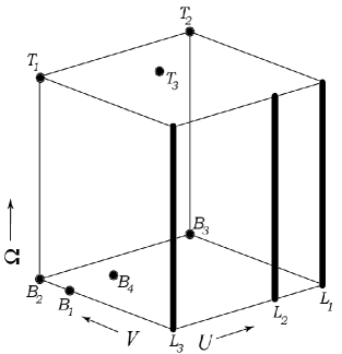
Figure 1: The compact state space for the dynamical system (8) with equilibrium points. The position of $B_{1}$ and $B_{4}$ depends on $n_{0}$ ($B_{4}$ is only present for $n_{0}>3$) and the position of $T_{3}$ depends on $\gamma_{1}$.

We observe that all six faces of the cube are invariant subspaces. On each of the four side faces, the induced dynamical system possesses a simple structure; the orbits on the side faces are depicted in Fig. 2.

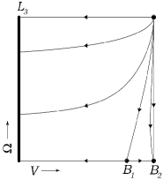
(a) $U=0$

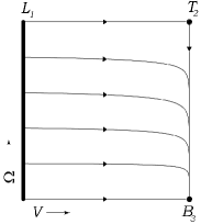
(b) $U=1$

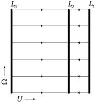
(c) $V=0$

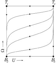
(d) $V=1$

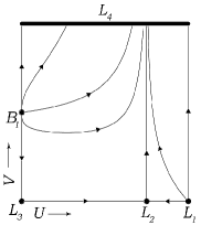
(e) $n_{0}=0$

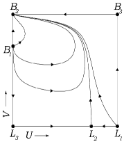
(f) $0<n_{0}\leq 3$

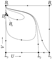
(g) $3<n_{0}\leq(11+8\sqrt{2})/7$

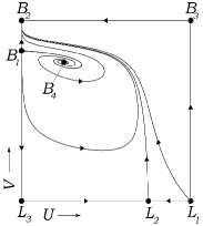
(h) $(11+8\sqrt{2})/7<n_{0}\leq 5$

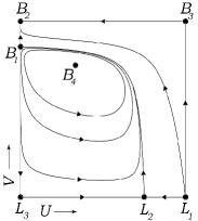
(i) $n_{0}=5$

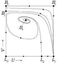
(j) $n_{0}>5$

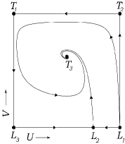
(k) $\gamma_{1}=1.1$

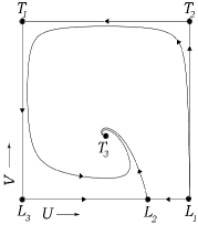
(l) $\gamma_{1}=1.9$

Figure 2: In (a), (b), (c), and (d) orbits for the four side faces are shown. The $U=0$, $U=1$, and $V=1$ faces involve $\sigma$ and $\Upsilon$, which depend on the equation of state. For the plots the relativistic polytrope with $\Gamma=4/3$ has been chosen; however, the qualitative structure is the same for all equations of state. In (e), (f), (g), (h), (i), and (j) orbits on the Newtonian subset $\Omega=0$ for different $n_{0}$ are presented. The subfigures (k) and (l) show orbits on the $\Omega=1$ subset for some values of $\gamma_{1}$.

The dynamical system on the $\Omega=0$ subset is in fact Newtonian, cf. Appendix A: since $\sigma=0$ on $\Omega=0$, $U$ and $V$ coincide with Newtonian homology variables and thus the system represents the Newtonian homology invariant equations for an exact polytrope with index $n_{0}$. On the $\Omega=0$ subset the flow of the dynamical system exhibits rather complicated features. In particular, $n_{0}$ serves as a bifurcation parameter: there exist bifurcations for $n_{0}=0$, $n_{0}=3$, and $n_{0}=5$, as indicated by the properties of the fixed points. The case $n_{0}=5$ is exactly solvable: the orbits can be represented implicitly by

$$\Phi=\sqrt{U}{V}^{3/2}(U(8-9\,V)+7\,V-6)-d(1-U)^{3/2}(1-V)^{5/2}=0\>,$$ (19)

where the parameter $d$ is required to satisfy $d\geq-9/8$. The fixed point $B_{3}$ is represented by $d=-9/8$; $-9/8<d<0$ defines a one-parameter family of closed orbits, which we will henceforth denote by $C$; $d=0$ characterizes the orbit that connects $L_{2}$ and $B_{1}$; the remaining orbits correspond to positive values of $d$, cf. Fig. 2(i). Typical orbits for a selection of values of $n_{0}$ are depicted in Fig. 2; cf. also the analogous non-compact figures in the standard literature, e.g., p.201 in [20].

The dynamical system on the $\Omega=1$ subset can be regarded as describing the relativistic scale-invariant equations for linear equations of state $p=(\gamma_{1}-1)\rho c^{2}$, a fact that reflects itself in the decoupling of the $(U,V)$-equations from the system (8) for purely linear equations of state. Typical orbits are depicted in Fig. 2 (cf. also, e.g., [3], where an analogous non-compact phase portrait is given).

The global dynamics of the dynamical system (8) is determined by the fixed points on the boundaries of the state space, which enables us to describe the asymptotics of the interior orbits. The statement is made precise in the following theorem.

Theorem 4.1.

The $\alpha$-limit of an interior orbit is a fixed point on $L_{1}$, $L_{2}$, or the fixed point $T_{3}$. The $\omega$-limit of an interior orbit is always located on $\Omega=0$, and it is one of the fixed points $B_{1}$, $B_{2}$, or $B_{4}$, when $n_{0}\neq 5$. If $n_{0}=5$, then the $\omega$-limit can also be an element of the 1-parameter set of closed orbits $C$.

Proof.

The proof of the theorem is based on the monotonicity principle [13]: if there exists a function $Z$ (defined on a closed, bounded, future (past) invariant set $S$) that is monotonic along the flow of the dynamical system $\dot{x}=f(x)$, then $\omega(S)$ ($\alpha(S)$) is contained in $\{x\in S|\dot{Z}=0\}$.

The function $\Omega$ is such a monotone function on the state space, i.e., $d\Omega/d\lambda<0$, except on $\Omega=0$, $\Omega=1$, and $V=0$. It follows that the $\omega$-limit of an interior orbit is located on $\Omega=0$ or $V=0$, while the $\alpha$-limit of an interior orbit must lie on $\Omega=1$ or $V=0$. However, it follows from the known orbit structure on $V=0$ and the local fixed point analysis that $V=0$ cannot possess an $\omega$-limit. Similarly, it follows that only $L_{1}$ and $L_{2}$ constitute $\alpha$-limits for interior orbits.

It remains to determine the $\omega$-limit ($\alpha$-limit) sets for interior orbits on $\Omega=1$ and $\Omega=0$. Again we make use of the monotonicity principle, however, to simplify the discussion we use the uncompactified variables $(u,v)$.

On $\Omega=1$, a monotone function is given by

$$Z_{3}=[-(\gamma_{1}-1)h_{1}(u,v)+3\gamma_{1}-2]^{2}(uv)^{-p_{1}}(1+2(\gamma_{1}-1)v)^{p_{1}-1}\ ,$$ (20)

where the non-negative function $h_{1}$ and the non-negative constant $p_{1}$ are defined by

$$h_{1}(u,v):=\gamma_{1}(1+(\gamma_{1}-1)u)v=-h|_{\Omega=1}\;,\qquad p_{1}=\frac{4(\gamma_{1}-1)^{2}}{\gamma_{1}(5\gamma_{1}-4)}\ .$$ (21)

Its derivative along orbits reads

$$\frac{dZ_{3}}{d\xi}=-\frac{p_{1}}{2}\,(3\gamma_{1}-2)(2-h_{1})^{2}[(\gamma_{1}-1)h_{1}+3\gamma_{1}-2]^{-1}Z_{3}\ .$$ (22)

Application of the monotonicity principle yields that only $T_{3}$ is a possible $\alpha$-limit set on $\Omega=1$.

We now turn our attention to the $\omega$-limit sets of interior orbits, which we have shown to lie on $\Omega=0$. For $n_{0}\leq 3$ the function $Z_{1}=uv^{3}$ is monotone along orbits, $dZ_{1}/d\xi=Z_{1}(2u+v(3-4\Upsilon_{0}))$. For $n_{0}>3$ define

$$Z_{2}=(uv)^{2/(n_{0}-1)}\left[\frac{n_{0}-5}{(n_{0}-1)^{2}}+\frac{2v}{(n_{0}+1)(n_{0}-1)}-\frac{v^{2}}{2(n_{0}+1)^{2}}-\frac{uv}{(n_{0}+1)^{2}}\right]\ ,$$ (23)

and observe that $dZ_{2}/d\xi=(n_{0}-5)\,(n_{0}+1)^{-2}(n_{0}-1)^{3}((uv)^{2/(n_{0}-1)}\big{(}2(n_{0}+1)-(n_{0}-1)v\big{)}^{2}$, i.e., $Z_{2}$ is monotonic on orbits for $3<n_{0}\neq 5$. (Note that the flow is non-vanishing on $v=2(n_{0}+1)/(n_{0}-1)$ except for at $B_{4}$.) Thus, by the monotonicity principle, taking also the solution structure on the boundaries into account, only the fixed points $B_{1}$, $B_{2}$, $B_{4}$ can serve as $\omega$-limit sets on $\Omega=0$. The exceptional case is $n_{0}=5$: then there also exists a 1-parameter family, $C$, of closed orbits (periodic solutions) described by (23) (see also (19)), which acts as an $\omega$-limit set for interior solutions.  

Theorem 4.2.

If $0<n_{0}\leq 3$ $(n_{0}=0)$, then all orbits end at $B_{2}$ $(L_{4})$.

Proof.

We distinguish two cases, $n_{0}<3$ and $n_{0}=3$. For $n_{0}<3$ the proof is trivial; each interior orbit converges to $B_{2}$ for $0<n_{0}<3$ (to $L_{4}$ when $n_{0}=0$), which follows from the proof of Theorem 4.1 and the local dynamical systems analysis (Table 1).

In the case $n_{0}=3$, $B_{1}$ is not hyperbolic. Nevertheless, by applying center manifold theory, we show that no interior orbit converges to $B_{1}$ as $\lambda\rightarrow\infty$:

It is advantageous to investigate the problem in adapted uncompactified variables $\{x\geq 0,y,z\geq 0\}$, defined by

$$u=x(n_{0}-2)/(n_{0}+1)\qquad v=(n_{0}+1)-x+y\qquad\omega=z\>,$$ (24)

The fixed point $B_{1}$ is represented by $(0,0,0)$ and the dynamical system (6) reads

$$\begin{array}[]{lcl}\dot{x}=&&+\quad N_{x}(x,y,z)\\[3.0pt] \dot{y}=&y&+\quad N_{y}(x,y,z)\\[3.0pt] \dot{z}=&-f_{0}(1+n_{0})z&+\quad N_{z}(x,y,z)\>,\end{array}$$ (25)

where $N_{x}$, $N_{y}$, $N_{z}$ denote the nonlinear terms. $N_{x}$ is given by

$$N_{x}=x(3-4\Upsilon(z)-x/4+(x-y)\Upsilon(z))+C_{1}(x,y,z)\sigma(z)+C_{2}(x,y,z)\sigma^{2}(z)\>.$$ (26)

A center manifold of the system (25), i.e., an invariant manifold tangential to the center subspace at the fixed point, is represented by $\{(x,h_{y}(x),h_{z}(x))|0\leq x<\varepsilon\}$ satisfying

$$\partial_{x}h_{y}(x)\;\dot{x}(x,h_{y}(x),h_{z}(x))=\dot{y}(x,h_{y}(x),h_{z}(x))\qquad\partial_{x}h_{z}(x)\;\dot{x}(x,h_{y}(x),h_{z}(x))=\dot{z}(x,h_{y}(x),h_{z}(x))\>,$$ (27)

and the tangency conditions $h(0)=0$, $\partial_{x}h(0)=0$. We obtain

$$h_{y}(x)=-x^{2}/2-x^{3}+O(x^{4})\qquad h_{z}(x)\equiv 0\>.$$ (28)

Note in particular that the center manifold lies in the Newtonian subset of the state space. The center manifold reduction theorem states that the flow of the full nonlinear system is locally equivalent to the flow of the reduced system (see, e.g., [9])

$$\begin{array}[]{lcl}\dot{x}&=&N_{x}(x,h_{y}(x),h_{z}(x))=x^{2}/2+O(x^{3})\\[3.0pt] \dot{y}&=&y\\[3.0pt] \dot{z}&=&-f_{0}(1+n_{0})z\>.\end{array}$$ (29)

The flow given by (29) clearly prevents interior solutions $(x>0,y,z>0)$ from converging to $B_{1}$, which proves the claim.  

Collecting the results of the local and global dynamical systems analysis yields the following. Interior orbits originate from $L_{1}$ (a two-parameter set); $L_{2}$ (a one-parameter set); and $T_{3}$ (a single orbit). They end at $B_{1}$ (when $n_{0}>3$; a one-parameter set); $B_{2}$ (a two-parameter set); $L_{4}$ (when $n_{0}=0$; a two-parameter set); $B_{4}$ (when $n_{0}>3$; a single orbit when $n_{0}\leq 5$ and a two-parameter set when $n_{0}>5$); and at the periodic curves $C$ (when $n_{0}=5$; a two-parameter set).

An orbit in the state space corresponds to a perfect fluid solution. Note that the perfect fluid solution is only represented in that range of $r$ where $p>0$, i.e., the fluid body, and where $m>0$; cf. Sec. 2. If the configuration has a finite radius $R$, then the fluid solution is joined to a vacuum solution, a Schwarzschild solution, at $r=R$.

The one-parameter set of regular perfect fluid solutions, i.e., solutions of (3) with a regular center of spherical symmetry, appears in the state space as the one-parameter set of orbits that originate from $L_{2}$. When $d\rho/dp\geq 0$ is assumed, $\rho(r)\leq\bar{\rho}(r)$ holds for regular solutions, where $\bar{\rho}=3m/(4\pi r^{3})$ is the “average density”. Translated to the state space variables we obtain $U\leq 3/4$. In order to show this inequality within the dynamical systems framework, consider the surface $U=3/4$ and the flow through this surface: $dU/d\lambda|_{U=3/4}=-3\Upsilon(1+\sigma)(1+3\sigma)V/64\leq 0$, since $\Upsilon\geq 0$ when $d\rho/dp\geq 0$. Hence, $U=3/4$ acts as a “semi-permeable membrane” for the flow of the dynamical system. By noting that the unstable subspaces at $L_{4}$ are characterized by $U\leq 3/4$ the claim is established.

If a perfect fluid solution satisfies $1-2Gm/(rc^{2})>0$ initially at $r=r_{0}$ for initial data $(m_{0},p_{0})$, then this condition holds everywhere. For a proof (involving regular solutions) see, e.g., [1]. In the state space picture this result can be established quite easily. By construction, the initial data is a point in the interior of the state space and the orbit passing through this point represents the associated perfect fluid solution. Since $V<1$ for the orbit, we obtain that

$$1-\frac{2Gm}{rc^{2}}=\frac{1-V}{1-V+2\sigma V}>0$$ (30)

holds everywhere within the fluid body. We can even show that $1-2Gm/(rc^{2})\geq const>0$ for all $r$: the considered orbit can have three possible end points; suppose that the orbit ends in the fixed point $B_{2}$, which is the only non-trivial case since then $V\rightarrow 1$ when $\lambda\rightarrow\infty$. We will see in the subsequent section that such an orbit gives rise to a perfect fluid solution possessing a finite radius $R$ and a total mass $M$, which are related by $GM/(Rc^{2})=B/(2B+s)$, where $B$ and $s$ are positive numbers. Hence the claim is established.

By introducing the function

$$\Psi_{1}:=1-\frac{(3{\cal M}+{\cal P})^{2}}{2(2{\cal M}+{\cal P})}\ ,$$ (31)

where

$${\cal M}:=\frac{Gm}{c^{2}r}=\frac{\sigma(\Omega)V}{1-V+2\sigma V}\,;\quad{\cal P}:=\frac{4\pi G}{c^{4}}r^{2}p=\left(\frac{U}{1-U}\right)\left(\frac{\sigma^{2}V}{1-V+2\sigma V}\right)\ ,$$ (32)

we can write the relativistic Buchdahl inequality as

$$\Psi_{1}\geq 0\ .$$ (33)

Note that the surface inequality ${\cal M}\leq 4/9$ is obtained by setting ${\cal P}=0$. The flow on the surface $\Psi_{1}=0$ is given by

$$\frac{d\Psi_{1}}{d\lambda}=\frac{\sigma(3-4U)(1-U+\sigma U)^{3}V}{(2(1-U)+\sigma U)^{2}(3(1-U)+\sigma U)}$$ (34)

and hence, since $U\leq 3/4$ for regular solutions, it follows that the derivative is positive (zero) when $U<3/4$ ($U=3/4$). The Buchdahl surface $\Psi_{1}=0$ and the $U=3/4$ surface are depicted in Fig. 3 for the relativistic polytropes with $\Gamma=3/4$ and $\Gamma=2$ (note that the Buchdahl-surface is affected by the equation of state through $\sigma(\Omega)$). Since regular solutions start at $V=0$ and since the flow on the Buchdahl surface is directed toward $V=0$, the regular solutions cannot pass through the Buchdahl-surface. Hence, for regular solutions only a limited part of the state space is accessible (cf. Fig. 3). This constitutes the dynamical systems proof of the Buchdahl inequality.

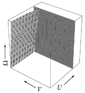
(a) $\Gamma=3/4$

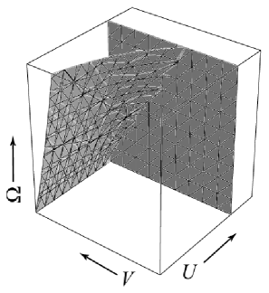
(b) $\Gamma=2$

Figure 3: The Buchdahl surface $\Psi_{1}=0$ for the relativistic polytrope together with the surface $U=3/4$.

5 Translating the state space picture to a physical picture

In this section we translate the state space picture to the common physical variables. To this end recall, firstly, that an orbit in the interior of the state space stands for a fluid solution $(m(r),p(r),\rho(r))$ ($r>0$) inside the fluid body via the transformation (5). Secondly, consider the following auxiliary equations:

$$\frac{dr}{d\lambda}=(1-U)(1-V)r\quad,\qquad\frac{dm}{d\lambda}=U(1-V)m$$ (35a)

$$\frac{dp}{d\lambda}=-(1+\sigma)V(1-U+\sigma U)p\quad,\quad\frac{d\sigma}{d\lambda}=-(1+\sigma)(1-\Upsilon)V(1-U+\sigma U)\sigma$$ (35b)

$$\frac{Gm}{c^{2}r}=\frac{\sigma V}{1-V+2\sigma V}$$ (35c)

$$r^{2}=\frac{c^{2}}{4\pi G}\left(\frac{U}{1-U}\right)\left(\frac{\sigma V}{1-V+2\sigma V}\right)\rho(\Omega)^{-1}$$ (35d)

$$m^{2}=\frac{c^{6}}{4\pi G^{3}}\left(\frac{U}{1-U}\right)\left(\frac{\sigma V}{1-V+2\sigma V}\right)^{3}\rho(\Omega)^{-1}\>.$$ (35e)

Based on an equation of state in explicit form (9), i.e., $k\rho c^{2}=\psi(kp)$, and a pressure variable $\omega=\omega(kp)$ we can replace $\rho^{-1}$ in the last two equations by

$$\rho^{-1}=\frac{kc^{2}}{\psi(\Omega)}\qquad\mbox{or}\qquad\rho^{-1}=kc^{2}\sigma(\Omega)\,\frac{1}{(kp)(\Omega)}\>,$$ (36)

where $(kp)(\Omega)=\Omega^{1/a}/(1-\Omega)^{1/a}$ in the case $\omega=(kp)^{a}$.

Equations (35a) can be used to obtain an intuitive picture of where solutions gain mass and radius in the state space. Since these equations are independent of $\Omega$, it is possible to visualize $d\ln m/d\lambda$ and $d\ln r/d\lambda$ as contour plots on the $U,V$ plane, see Fig. 4. The picture suggests that no mass is acquired near the side faces $U=0$ and $V=1$, and hence the fixed points $B_{1}$ and $B_{2}$ (and $L_{5}$, if present) are attractors for solutions with finite masses. In contrast, $d\ln r/d\lambda$ does not vanish near $B_{1}$, but only near $B_{2}$ (and $L_{5}$, if present). Therefore, $B_{2}$ is the only attractor for solutions with finite radii. Solutions converging to $B_{3}$ (or to a periodic orbit $C$ when $n_{0}=5$) for $\lambda\rightarrow\infty$ acquire both infinite masses and radii.

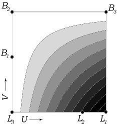
(a) $\frac{\ln m}{d\lambda}$

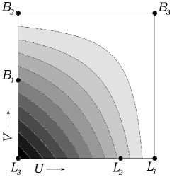
(b) $\frac{\ln r}{d\lambda}$

Figure 4: Contour plots of $\frac{\ln m}{d\lambda}$ and $\frac{\ln r}{d\lambda}$. The white regions correspond to the minimum value of the functions ($=0$) and the black to the maximum value ($=1$).

To obtain a rigorous derivation of the asymptotic mass and radius features of the various solutions we must combine equations (35) with the local dynamical systems analysis in the neighborhood of the fixed points (and the periodic orbits $C$ when $n_{0}=5$). We only state the results here (for a detailed discussion of the corresponding and rather similar Newtonian situation, see [11]):

Solutions that originate from: (i) $L_{1}$ are solutions with negative masses for small $r$; when they have acquired sufficient positive mass, so that the mass function $m$ has become zero, they appear in the state space through $L_{1}$, cf. the Newtonian case discussed in [11]); (ii) $L_{2}$ have a regular center and are therefore solutions of particular physical interest; (iii) $T_{3}$ have a non-regular center ($\rho\propto r^{-2}$ for $r\rightarrow 0$) and describe the limit when the central pressure goes to infinity. One can show that $T_{3}$ is associated with a self-similar solution admitting a $H_{4}$ spacetime transitive symmetry group. It is a special case of a solution found by Tolman [19], but has been rediscovered many times, see [16] and references therein.

Solutions that end at: (i) $B_{1}$ ($n_{0}>3$) have infinite radii but finite masses; (ii) $B_{2}$ and (iii) $L_{4}$ ($n_{0}=0$) have finite masses and radii and are therefore the most interesting solutions; (iv) $B_{4}$ ($n_{0}>3$) and (v) $C$ ($n_{0}=5$) have infinite radii and masses ($m(r)\sim r^{(n_{0}-3)/(n_{0}-1)}$ in the case of $B_{4}$).

Let us now take a closer look at the 2-parameter family of orbits that converges to $B_{2}$ as $\lambda\rightarrow\infty$. All such orbits correspond to perfect fluid solutions with finite radii $R$ and masses $M$. To describe the behavior of the physical observables as $r\rightarrow R$, we will use the local dynamical systems results together with equations (5), (7), or (35). Recall that the solutions of the dynamical system (8) with specified $\Upsilon(\Omega)$ and $\sigma(\Omega)$ represent the totality of perfect fluid solutions corresponding to a one-parameter family of equations of state, cf. (14). For $p\rightarrow 0$ the leading term of a considered equation of state was shown to be given by $k\rho c^{2}=s\,(kp)^{\Upsilon_{0}}$, where $s$ is a dimensionless constant, cf. (10).

The 2-parameter family of orbits that converges to $B_{2}$ can be conveniently characterized by the constants $A$ and $B$, defined according to

$$A:=\lim_{\lambda\rightarrow\infty}U(1-V)^{-n_{0}}\;,\quad B:=\lim_{\lambda\rightarrow\infty}\Omega^{\frac{1}{f_{0}(n_{0}+1)}}(1-V)^{-1}\;.$$ (37)

Expressed in these quantities we obtain the following, when $r\rightarrow R$,

$$p(r) =k^{-1}B^{n_{0}+1}\,\delta r^{n_{0}+1}+\frac{n_{0}+1}{n_{0}+2}\,k^{-1}B^{n_{0}+1}\left(2(n_{0}+1)+\frac{4\pi R^{3}}{Mc^{2}}\,k^{-1}B^{n_{0}+1}A^{-1}(3+2n_{0})\right)\delta r^{n_{0}+2}+O(\cdot)$$ (38a)

$$m(r) =M(1-A\delta r^{n_{0}+1})+O(\cdot)$$ (38b)

$$\rho(r) =\frac{1}{4\pi R^{3}}\,MA\,\delta r^{n_{0}}+O(\cdot)\,,$$ (38c)

where $\delta r=\frac{1}{n_{0}+1}\frac{R-r}{R}$.

The radius $R$ and mass $M$ for a solution are uniquely determined by the values of $A$ and $B$ through

$$R^{2}=\frac{kc^{4}}{4\pi s\,G}\>\frac{AB^{1-n_{0}}}{s+2B}\;,\quad\qquad M^{2}=\frac{kc^{8}}{4\pi s\,G^{3}}\>\frac{AB^{3-n_{0}}}{(s+2B)^{3}}\>.$$ (39)

The dimensionless quotient $GM/(c^{2}R)$ is given by $GM/(c^{2}R)=B/(s+2B)$, so that the line element (1) on the surface $r=R$ is determined by $e^{2\Lambda}=c^{-2}e^{-2\Phi}=1/(1-{\textstyle{\frac{2GM}{c^{2}R}}})=1+2B/s$. (Hence, naturally, $GM/(c^{2}R)$ can be used instead of $B$ together with $A$ to parameterize the different solutions.)

Eq. (39) and the related formulas are useful in, e.g., numerical computations, since it is fairly easy to compute $A$ and $B$. Below, in numerical applications, we are going to compare solutions with a reference solution, i.e., we are going to consider the dimensionless ratios $R/R_{\rm ref}$, $M/M_{\rm ref}$, where $R_{\rm ref}$ and $M_{\rm ref}$ are the radius and mass of a typical reference solution. Of course, the dimensional factors $(kc^{4})/(4\pi sG)$ and $(kc^{8})(4\pi sG^{3})$ drop out in this case.

For illustrative purposes consider cylindrical coordinates at $B_{2}$, i.e., the coordinate transformation $(U,V,\Omega)=(\varepsilon\sin\phi,1-\varepsilon\cos\phi,h^{a})$ with $0\leq\phi\leq\pi/2$, $0\leq h$, $0\leq\varepsilon$, which leads to

$$A=\lim_{\lambda\rightarrow\infty}\epsilon^{1-n_{0}}\sin\phi\,(\cos\phi)^{-n_{0}}\;,\quad B=\lim_{\lambda\rightarrow\infty}h^{1/(n_{0}+1)}\,(\epsilon\cos\phi)^{-1}\ .$$ (40)

As every orbit in a neighborhood of $B_{2}$ converges to $B_{2}$ as $\lambda\rightarrow\infty$, we obtain approximate expressions with arbitrary accuracy by choosing $\varepsilon$ sufficiently small. In this picture, every orbit is uniquely characterized by its intersection point $(h,\phi)$ with the small $\varepsilon$-cylinder, and accordingly these values uniquely determine $M$ and $R$ by combining (39) with (40). A similar discussion holds for $L_{4}$ when $n_{0}=0$; for the corresponding Newtonian discussion, see [11].

6 Mass-radius theorems

In this section we will prove several theorems concerning mass-radius properties of solutions, where we focus on regular solutions. The underlying equations of state are as always understood to be asymptotically polytropic for $p\rightarrow 0$ and asymptotically linear for $p\rightarrow\infty$, as discussed in Sec. 3.

Theorem 6.1.

All regular solutions have infinite masses and infinite radii if $\,\Gamma_{N}\leq\frac{6}{5}$ and $\sigma\leq 1$.

Proof.

Consider the function $\Psi_{2}(U,V,\Omega)$, defined by

$$\Psi_{2}:=U(8-9V)+7V-6\ .$$ (41)

The surface $\Psi_{2}=0$ coincides with the regular orbit from $L_{2}$ to $B_{1}$ for $n_{0}=5$ when projected onto the $\Omega=0$ plane, cf. (19). Taking the derivative of this function and evaluating it on the surface $\Psi_{2}=0$ yields

$$\frac{d\Psi_{2}}{d\lambda}=V(1-V)\,\left(\,(5-6\Upsilon)(1-U)^{2}+2\,\sigma\,((4U+U\sigma-1)(3-4U)-3\Upsilon(1-U)(1+U\sigma))\,\right)\ .$$ (42)

When $\Gamma_{N}\leq\frac{6}{5}$ ($\Upsilon\geq\frac{5}{6}$) and $\sigma\leq 1$, then $d\Psi_{2}/d\lambda<0$. Since in addition the unstable subspaces of the fixed points $L_{2}$ lie in the region $\Psi_{2}<0$ of the state space, it follows that a regular orbit can never leave this region. The only attractor in this part of the state space is the fixed point $B_{4}$, cf. Theorem 4.1. Since $B_{4}$ gives rise to perfect fluid solutions with infinite masses and radii the claim of the theorem is established.  

Remark.

The assumption $\sigma\leq 1$ is just the dominant energy condition, and is satisfied, e.g., for causal relativistic polytropes. In the theorem, the condition $\sigma\leq 1$ is a sufficient but not necessary; the statement is valid for much larger $\sigma$, but not for arbitrarily large values.

Let us define $\sigma_{l}:=\left(-4+\sqrt{16+2\,(5\Gamma_{N}-6)}\,\right)/6$.

Theorem 6.2.

All regular solutions with $\Omega_{c}\in(0,\Omega_{\rm max})$ have finite masses and radii if $\Gamma_{N}>\frac{6}{5}$ and if $\sigma<\sigma_{l}$ on $(0,\Omega_{\rm max})$.

Proof.

Consider again the function $\Psi_{2}$ as defined in (41). If $\Gamma_{N}>6/5$ (i.e., $\Upsilon<5/6$), then $d\Psi_{2}/d\lambda>0$ is satisfied, provided that $\sigma<\sigma_{l}$. Under the same conditions, the unstable subspace of a fixed point on $L_{2}$ lies in the region $\Psi_{2}>0$. It follows that a regular orbit, which originates from a fixed point $(3/4,0,\Omega_{c})$ on $L_{2}$, is confined to the region $\Psi_{2}>0$ of the state space, if $\sigma(\Omega)<\sigma_{l}$ for all $\Omega\leq\Omega_{c}$. The only attractor in the region $\Psi_{2}>0$ is the fixed point $B_{2}$, and since $B_{2}$ generates solutions with finite masses and radii, the theorem is established.  

Remark.

In [1] it is shown that if $6/5<\Gamma_{0}<2$ then the solution possesses a finite radius provided that $\sigma$ is sufficiently small (Theorem 4, p.994). In [28] and [10] theorems related to Theorem 6.2 are proved with completely different methods. In the above theorem, the lower limit for $\sigma$ is not a particularly good lower bound for “most” equations of state. Indeed, as follows from the next theorem, when $n_{0}\leq 3$, then all solutions have finite masses and radii for all $\Omega_{c}\in[0,1]$ and thus all values of $\sigma$ are allowed.

Theorem 6.3.

(Finiteness of perfect fluid solutions). All regular and non-regular perfect fluid solutions have finite radii and masses if $n_{0}\leq 3$ (i.e., $\Gamma_{0}\geq 3/4$).

Proof.

This theorem follows from Theorem 4.2, which shows that all solutions end at $B_{2}$ if $n_{0}\leq 3$ (at $L_{4}$ if $n_{0}=0$), and from that $B_{2}$ ($L_{4}$) is associated with solutions with finite masses and radii.  

Remark.

(General validity). The last theorem holds irrespective of the asymptotic behavior of the equation of state at high pressures. Also for the first two theorems the asymptotic high pressure regime is irrelevant if one restricts the attention to solutions with finite central pressures. This is because the proofs in such cases do not rely on the inclusion of the boundary $\Omega=1$ in the state space. This is in contrast to the next theorem which makes use of the $\Omega=1$ subset and relies on our assumptions about differentiability of the equation of state when $\Omega\rightarrow 1$ ($p\rightarrow\infty$).

Theorem 6.4.

(Spiral structure of the $(M,R)$-diagram). Let $0<n_{0}\leq 3$. For sufficiently high central pressures the mass-radius diagram exhibits a spiral structure, i.e., $(R(p_{c}),M(p_{c}))$ is given by

$$\left(\begin{array}[]{c}R(p_{c})\\ M(p_{c})\end{array}\right)\>=\>\left(\begin{array}[]{c}R_{O}\\ M_{O}\end{array}\right)\>+\>\left(\frac{1}{p_{c}}\right)^{\tau_{1}}\>{\mathcal{B}}\>{\mathcal{J}}(\tau_{2}\log p_{c}\,)\>b\>+\>o(\left(\frac{1}{p_{c}}\right)^{\tau_{1}})\>,$$ (43)

where $R_{O}$ and $M_{O}$ are constants, ${\mathcal{B}}$ is a matrix with positive determinant, and $b$ a non-zero vector. The matrix ${\mathcal{J}}(\varphi)\in\mathrm{SO}(2)$ describes a (positive) rotation by an angle $\varphi$, and the constants $\tau_{1}$ and $\tau_{2}$ are given by

$$\tau_{1}=\frac{3\gamma_{1}-2}{4\gamma_{1}}\,,\qquad\tau_{2}=\frac{1}{4\gamma_{1}}\,\sqrt{c}\>,$$ (44)

where $\sqrt{c}=\sqrt{-36+44\gamma_{1}-\gamma_{1}^{\>2}}$ see Table 1.

Sketch of proof. The basic observation is that the regular orbit on $\Omega=1$ forms a spiral as it converges to $T_{3}$, and that this spiral subsequently reflects itself as a spiral in the $(R,M)$-diagram.

Choose $\varepsilon$ small and set $\omega_{\varepsilon}=1-\varepsilon$. The dynamical system asymptotically decouples as $\Omega\rightarrow 1$ (recall from (12) and (13) that we can always choose $\omega$ in such a way that $\frac{d\Upsilon}{d\Omega}=O((1-\Omega)^{k})$ and $\frac{d\sigma}{d\Omega}=O((1-\Omega)^{k})$ as $\Omega\rightarrow 1$), which enables us to approximately solve the system on $[0,1]^{2}\times[\Omega_{\varepsilon},\Omega]$: let $U_{\mathrm{L}}(\lambda)$, $V_{\mathrm{L}}(\lambda)$ denote the regular solution of the system (8a) and (8b) with $\Gamma_{N}=1$, $\sigma=\sigma_{1}=\gamma_{1}-1$. Then $(U_{\mathrm{L}}(\lambda),V_{\mathrm{L}}(\lambda),\Omega(\lambda))$ is an approximate solution of (8) when $\frac{d\Omega}{d\lambda}=-f_{1}(1-\Omega)H_{\mathrm{L}}$, where $H_{\mathrm{L}}=H(U_{\mathrm{L}},V_{\mathrm{L}},1)$.

For large $\lambda$ the orbit $(U_{\mathrm{L}}(\lambda),V_{\mathrm{L}}(\lambda))$ has the form of a spiral, i.e.,

$$\left(\begin{array}[]{c}U_{\mathrm{L}}(\lambda)\\ V_{\mathrm{L}}(\lambda)\end{array}\right)\>=\>\left(\begin{array}[]{c}U_{T_{3}}\\ V_{T_{3}}\end{array}\right)+\exp(-\delta_{1}\lambda)\>{\mathcal{B}}^{\prime}\>{\mathcal{J}}(\delta_{2}\lambda)\>b^{\prime}\>,$$ (45)

where $U_{T_{3}},V_{T_{3}}$ are the coordinates of the fixed point $T_{3}$; ${\mathcal{B}}^{\prime}$ is a matrix with $\det{\mathcal{B}}^{\prime}>0$, and $b^{\prime}$ a non-zero vector; $\delta_{1}=\frac{\gamma_{1}}{4(\gamma_{1}^{2}+2)}(3\gamma_{1}-2)$ and $\delta_{2}=\frac{\gamma_{1}}{4(\gamma_{1}^{2}+2)}\,\sqrt{c}$. The constants $\delta_{1}$ and $\delta_{2}$ are the real and imaginary part of the complex eigenvalue that is associated with $T_{3}$, cf. with Table 1.

Inserting (45) into the equation for $\Omega$ we obtain the approximation

$$1-\Omega(\lambda)=(1-\Omega_{c})\,const\,\exp\big{(}f_{1}H_{T_{3}}\,(\lambda-\tilde{\lambda})\big{)},$$ (46)

where $H_{T_{3}}=H(U_{T_{3}},V_{T_{3}},1)=\gamma_{1}^{2}/(2+\gamma_{1}^{2})$, and $\tilde{\lambda}$ and $const$ are independent of $\Omega_{c}$ (the value of $\Omega(\lambda)$ as $\lambda\rightarrow-\infty$).

Consider the orbit that originates from $T_{3}$ into the state space: it intersects the plane $\Omega=\Omega_{\varepsilon}$ in a point $I$ with approximately the same $(U,V)$-coordinates as $T_{3}$. A regular solution with $\Omega_{c}$ sufficiently close to $1$ can be described by (45) and (46). It intersects $\Omega=\Omega_{\varepsilon}$ at $\lambda=\lambda_{c}$, where

$$\lambda_{c}=\frac{1}{aH_{T_{3}}}\,\log\frac{1}{1-\Omega_{c}}+const=\frac{1}{H_{T_{3}}}\log p_{c}+const\>.$$ (47)

For the components $(U(\lambda_{c}),V(\lambda_{c}))$ of this regular solution we have $(U(\lambda_{c}),V(\lambda_{c}))=(U_{T_{3}},V_{T_{3}})+(\delta U_{0},\delta V_{0})$ with

$$\left(\begin{array}[]{c}\delta U_{0}(\eta_{c})\\ \delta V_{0}(\eta_{c})\end{array}\right)\>=\>\left(\frac{1}{p_{c}}\right)^{\tau_{1}}\>{\mathcal{B}}^{\prime\prime}\>{\mathcal{J}}(\tau_{2}\log p_{c}\,)\>b^{\prime\prime}\>,$$ (48)

where ${\mathcal{B}}^{\prime\prime}$ ($\det{\mathcal{B}}^{\prime\prime}>0$) and $b^{\prime\prime}$ have absorbed the constants. From (48) we see that the set of regular solutions intersects $\Omega=\Omega_{\varepsilon}$ in a spiral in a neighborhood $U_{I}$ of $I$ in this plane.

The orbit that originates from $T_{3}$ and passes through $I\in U_{I}$ eventually intersects the mass-radius cylinder (cf. (40)) at some point $O\in U_{O}\subseteq\mathrm{cylinder}$, where the cylindrical coordinates of $O$ determine the mass $M_{O}$ and the radius $R_{O}$ of the solution (cf. (39)). The flow of the dynamical system induces a diffeomorphism $U_{I}\rightarrow U_{O}$, so that the spiral (48) in $U_{I}$ is mapped to a distorted (positively oriented) spiral in $U_{O}$. Since the cylindrical coordinates $(\phi,h)$ in the small neighborhood $U_{O}$ are related to $(R,M)$ by a positively oriented linear map, the spiral (48), with different ${\mathcal{B}}$ and $b$, appears also in the $(R,M)$ diagram.  

Remark.

Note that the theorem does not rely on the behavior of the equation of state in the intermediate non-asymptotic regimes. Hence the theorem describes a universal phenomenon and connects it with the self-similar solution that corresponds to $T_{3}$. A similar theorem has been proved in [24] using quite different methods. However, an advantage with the present approach, apart from less restrictive assumptions, brevity of proof, and clarity, is that it visually shows the importance of key solutions like the self-similar one associated with $T_{3}$.

7 Examples

In this section the dynamical systems approach to relativistic stellar models will be illustrated by several examples. The presented results also demonstrate the usefulness of the new framework in numerical computations.

7.1 Relativistic polytropes

As discussed in Sec. 3, a relativistic polytrope with index $\Gamma$ can be described by the dynamical system (8) with $\sigma=(\Gamma-1)\Omega$ and $\Upsilon=(1+(\Gamma-1)\Omega)/\Gamma$. The numerical integration of this system is straight forward, when we use the local analysis near the fixed points. The radius $R$ and the total mass $M$ of a solution can be obtained by various methods, in particular one can use equations (35d) and (35e), or one can include the auxiliary equations (35a) in the numerical integration of the dynamical system; Eq. (39) provides a different approach. Mass-radius diagrams for the regular solutions associated with different values of $\Gamma$ are shown in Fig. 5.

The theorems of Sec. 6 guarantee that all regular solutions possess finite $R$ and $M$ for $n_{0}\leq 3$ ($\Gamma\geq 4/3$). For $5>n_{0}>3$ ($\Gamma<4/3$), regular solutions with small central pressures must be finite fluid bodies. The numerical investigation improves these results: all regular solutions associated with $\Gamma\gtrsim 1.2971$ ($n_{0}\lesssim 3.366$) possess finite $R$ and $M$. A similar analysis was performed in [27] for purely polytropic equations of state: for a polytropic index $n\lesssim 3.339$ only finite fluid bodies appear. For an extensive discussion of the methods involved in establishing these results we refer the reader to that paper.

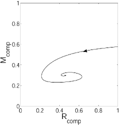
(a) $\Gamma=4/3$

(b) $\Gamma=5/3$

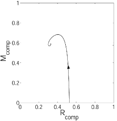
(c) $\Gamma=2.0$

Figure 5: Mass-radius diagrams for the regular relativistic polytropes. We display the compactified quantities $M_{{\rm comp}}=(M/M_{{\rm ref}})/(1+M/M_{{\rm ref}})$ and $R_{{\rm comp}}=(R/R_{{\rm ref}})/(1+R/R_{{\rm ref}})$, where $M_{{\rm ref}}$ and $R_{{\rm ref}}$ are typical values. The arrows indicate the direction of increasing $\Omega_{c}$, i.e., increasing central pressures.

Letting $\Gamma\rightarrow 1$ for relativistic polytropes implies that $\sigma\rightarrow 0$, and hence the dynamical system (8) approaches the Newtonian system, cf. Appendix A. Moreover, the equation for $\Omega$ decouples from the $U$- and $V$-equations, and the flows on the $\Omega=0$ and the $\Omega=1$ subset coincide in the limit. It follows that the regular surface is a surface perpendicular to the $\Omega=const$ plane; its projection to $\Omega=const$ is depicted in Fig. 6(c). Note also that the limit $\Gamma\rightarrow 1$ reveals a relationship between the Newtonian self-similar solution associated with $B_{4}$ (discussed, e.g., in [21]) and the relativistic self-similar solution associated with $T_{3}$.

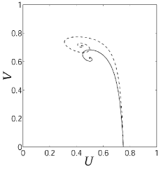
(a) $\Gamma=1.1$

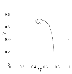
(b) $\Gamma=1.01$

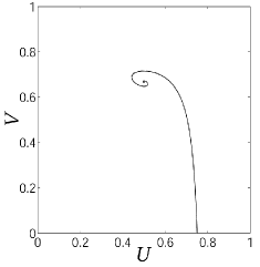
(c) $\Gamma=1.001$

Figure 6: Superimposed regular orbits for the relativistic polytrope, with varying $\Gamma=\Gamma_{0}=\gamma_{1}$. The dashed line corresponds to the orbit in the $\Omega=0$ plane and the solid line to the orbit in the $\Omega=1$ plane.

Regular solutions associated with an equation of state characterized by an arbitrary adiabatic index $\Gamma(p)$ close to $1$ lie close to the regular ”soft-limit-surface”. Hence, deviations from the soft-limit-surface measure both deviations of the equation of state from the soft limit and relativistic effects. Stiffer models are located ”further out” compared to the soft-limit-surface and increasing stiffness implies that the $U=3/4$ surface is approached, and it is on this “stiff-limit-surface” the incompressible perfect fluid solutions reside, as discussed previously. Note also that the Buchdahl surface, depicted in Fig. 3, for increasingly soft equations of state moves toward the $V=1$ surface, thereby becoming increasingly less restrictive. This illustrates that the Buchdahl inequality is a purely relativistic effect, since the surface disappears from the interior state space in the soft, and thereby Newtonian, limit.

7.2 The ideal neutron gas

The equation of state of the ideal neutron gas provides a simple model for neutron star matter; it is given in implicit form in equation (18). As discussed in Sec. 3, the ideal neutron gas can be naturally described in the dynamical systems framework, and is easy to handle numerically.

In Fig. 7 regular orbits for various values of $\Omega_{c}$ and the regular orbits on $\Omega=0$ and $\Omega=1$ are depicted.

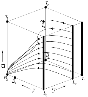
Figure 7: Typical regular orbits for the ideal neutron gas together with the orbits on the boundaries $\Omega=0$ and $\Omega=1$.

7.3 Composite equations of state

Consider first a stiff perfect fluid characterized by the equation of state $p=(\rho-\rho_{-})c^{2}$, which can be rewritten as

$$k\rho c^{2}=1+kp\>,$$ (49)

where $k=(\rho_{-}c^{2})^{-1}$. If we choose $\omega=kp$, we obtain $f=1$, $\Upsilon=\Omega$, and $\sigma=\Omega$, i.e., the dynamical system (8) becomes very simple. In this context, it is of interest to note that the solution that corresponds to the orbit from $T_{3}$ to $L_{4}$ (which is a solution with finite radius and mass but infinite central pressure) is explicitly known: it is a special case of a Tolman solution [19]. In the present formalism, the corresponding orbit is given by $U=3/(5+\Omega)$ and $V=(2+\Omega)/(2+3\Omega+4\Omega^{2})$. (For interesting features of this solution, see [17].)

As an example of a composite equation of state, let us continuously join a stiff equation of state $p=(\rho-\rho_{-})\,c^{2}$ (when $p>p_{j}$) to a relativistic polytrope (when $p<p_{j}$). Such an equation of state possesses a kink at $p_{j}$.

As outlined in Sec. 3, we work with two state spaces and dynamical systems, one pertaining to the relativistic polytrope and one representing the stiff fluid. The jump at $p_{j}$ reflects itself in a map between the two state spaces. Since $\rho$ is continuous, the values of $U,V$ are continuous under the map, however, there is a jump in $\Omega$. Since $\rho_{{\rm relpol}}(p_{j})=\rho_{{\rm stiff}}(p_{j})$ we have

$$\frac{1}{\Gamma-1}\,\left(\frac{(kp_{j})^{1/\Gamma}}{k}+p_{j}\right)=\rho_{-}c^{2}+p_{j}\>.$$ (50)

Dividing by $p_{j}$ and using that $\omega_{{\rm relpol}}(p)=(kp)^{(\Gamma-1)/\Gamma}$ and $\omega_{{\rm stiff}}(p)=(\rho_{-}c^{2})^{-1}p$, we obtain that

$$\Omega_{{\rm relpol}}=\frac{\Omega_{{\rm stiff}}}{\Gamma-1}$$ (51)

at the jump. If $\Gamma=2$, i.e., if the relativistic polytrope is asymptotically stiff, then there is no jump at all. A typical solution with a jump is illustrated in Fig. 8.

Note that, in general, if one starts with a regular solution in the first state space, then this solution has to be matched with a non-regular one associated with the other (extended) equation of state in the second state space.

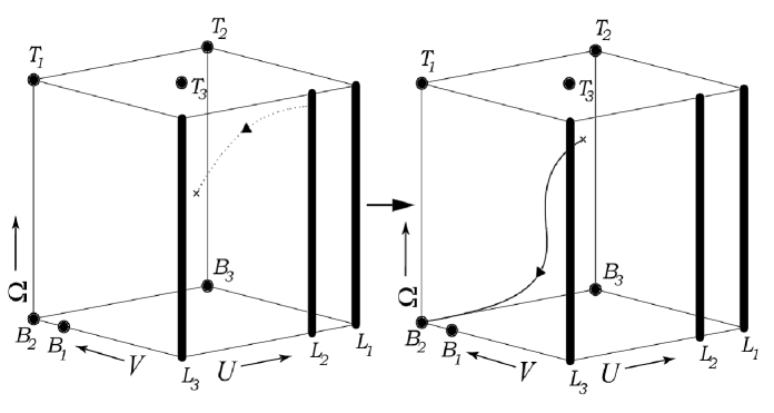
Figure 8: An example of an orbit for a composite equation of state consisting of a relativistic polytrope ($\Gamma=11/6$) and a stiff fluid. We have chosen to cut the ”stiff fluid orbit” at $\Omega=0.50$ (where $(U,V)=(0.58,0.60)$). The jump transformation law then yields a map to the point $(U,V,\Omega)=(0.58,0.60,0.75)$ in the state space of the relativistic polytrope, which serves as initial data for the subsequent evolution in that state space.

8 Concluding remarks

In this paper we have derived a dynamical systems formulation for the study of spherically symmetric relativistic stellar models. The method of ”homology invariants” known from the theory of Newtonian polytropes has been generalized both to a general relativistic context and to the broad class of asymptotically polytropic/linear equations of state. For previous related work see [11] (Newtonian asymptotic polytropes) and [27] (polytropes in GR).

The present formulation has turned out to be advantageous in many respects: (i) it provides a clear visual representation of the solution spaces associated with broad classes of equations of state; in particular it is revealed how the global qualitative properties of the solution space are influenced by the equation of state; (ii) the formulation makes the theory of dynamical systems available, which makes it possible to prove a number of theorems and describe the qualitative behavior of solutions; and (iii) the framework is particularly suited for numerical computations, since the numerics is supported by the local dynamical systems analysis.

The idea of using dimensionless variables and exploiting asymptotic symmetries and properties to derive a dynamical systems formulation is a quite versatile one. As another example, in a future paper, we will show how one also can treat a collisionless gas. The ”dynamical systems approach” can even be applied to problems, in general relativity and other areas, when no symmetries exist at all [4], as will be shown in another set of papers. Thus the ideas in the present work should be seen in a quite broad context, and it is likely that there are many problems in very different areas that could benefit from the type of ideas and the approach presented in this paper.

Acknowledgements

The authors would like to thank Alan Rendall and Robert Beig (J.M.H.) for helpful discussions. This work was supported by the DOC-program of the Austrian Academy of Sciences (J.M.H.) and the Swedish Research Council (C.U.).

Appendix A Appendix: Comparison with the Newtonian theory

The Newtonian equations of hydrostatic equilibrium are obtained from (2) and (3) by letting $c\rightarrow\infty$, however, note that in the Newtonian case $\rho$ is interpreted as the rest-mass density and $c^{2}\Phi\rightarrow\Phi_{N}$, the Newtonian potential. Consistently, since $\sigma=p/(\rho c^{2})$, in the dynamical system (8) we must set $\sigma\equiv 0$. Note also that $v$ reduces to $v=G\rho m/(rp)$. Since $\sigma\rightarrow 0$ for $p\rightarrow 0$, the relativistic system (8) and its Newtonian counterpart coincide on $\Omega=0$.

In the Newtonian case we can treat equations of state $\rho(p)$ with less restrictive asymptotic behavior in the regime $p\rightarrow\infty$. This is because it was the existence of $\sigma(\Omega)$ on the right hand side of the dynamical system that forced the assumption of asymptotic linearity upon us in the relativistic case. In particular we can naturally include asymptotically polytropic behavior as $p\rightarrow\infty$ in the Newtonian case (cf. [11]).

In Newtonian gravity there exist two independent dimensional scales, space and time, while in relativity, space and time are connected by the speed of light $c$, so that only one single dimensional scale remains. A Newtonian equation of state can be written in the implicit form

$$k_{1}p=\phi(\omega)\;,\qquad k_{2}\rho=\chi(\omega)\;,$$ (52)

where $\omega$ is a dimensionless variable and $k_{1}$ and $k_{2}$ are constants carrying the dimension $[p]^{-1}$ and $[\rho]^{-1}$ respectively; $\phi$ and $\chi$ are monotone functions in $\omega$ containing any number of dimensionless parameters. An explicit representation of (52) is $k_{2}\rho=\psi(k_{1}p)$.

Since our dynamical system is expressed in terms of purely dimensionless quantities, the dimensional parameters have to drop out. Consequently, a single dynamical system must be capable of describing the entire two-parameter set of equations of state (52) parameterized by $k_{1}$ and $k_{2}$. Indeed, the relevant function entering the dynamical system in the Newtonian case is $\Upsilon(\omega)$ given by $\Upsilon(\omega)=(d\ln\chi/d\ln\omega)(d\ln\phi/d\ln\omega)^{-1}$. Evidently, this function does not depend on $k_{1}$ and $k_{2}$. The same clearly holds for $f(\omega)=d\ln\phi/d\ln\omega$.

Example.

As an illustrative example, consider the equation of state $\rho=C_{1}p^{\Upsilon_{0}}+C_{2}p^{\Upsilon_{1}}$. By rescaling the equation and the two parameters one can write the equation of state as $k_{2}\rho=(k_{1}p)^{\Upsilon_{0}}+(k_{1}p)^{\Upsilon_{1}}$, and thus the equation has been brought to the desired form. The choice $\omega=(k_{1}p)^{a}$ ensures that $\Upsilon(\omega)$ and therefore also $\Upsilon(\Omega)$ are independent of $k_{1}$ and $k_{2}$, and interpolate monotonically between $\Upsilon_{0}$ and $\Upsilon_{1}$. In analogy to the detailed discussion in Sec. 3, the constant $a$ must be chosen sufficiently small so that a ${\mathcal{C}}^{1}$-differentiable dynamical system is obtained.

Remark.

(Consistent translatory invariance). As seen previously, it is the freedom to choose $\omega(p)$ that allows one to treat a one-parameter class of equations of state simultaneously by one specified dynamical system in the relativistic case. The freedom we were able to exploit in the Newtonian case to cover even two-parameter classes of equations of state reflects itself in the consistent translatory invariance of the Newtonian dynamical system. Namely, if ${\bf x}(\xi)$ (${\bf x}(\xi):=(u(\xi),v(\xi),\omega(\xi))$ (recall that $\xi=\ln r$) is a solution of the Newtonian dynamical system, then so is ${\bf x}_{0}:={\bf x}(\xi-\xi_{0})$, and moreover, the translated solution gives rise to a perfect fluid solution associated with an equation of state with the same $\Upsilon(p)$. In contrast, in the relativistic case this consistency is broken: if ${\bf x}(\xi)$ is a solution of the dynamical system (6), then so is ${\bf x}_{0}(\xi)={\bf x}(\xi-\xi_{0})$. However, whereas the solution ${\bf x}(\xi)$ can be consistently interpreted as a relativistic perfect fluid solution, associated with an equation of state $\rho(p)$ (determined by $\Upsilon$ and $\sigma$), this is not the case with the translated solution. Although the translated solution satisfies differential equations associated with $\rho(p)$, the initial data are not consistent with this equation of state. Accordingly, only one particular solution on every orbit of (6), can be interpreted as a relativistic perfect fluid solution. However, in the compactified dynamical system (8) this ‘defect’ is remedied by the appearance of the freedom in the new independent variable $\lambda$ (this ‘cure’ could also have been implemented in the $u,v,\omega$-formulation by defining $\xi$ through $dr/d\xi=r$, i.e, by letting $\xi=\ln r+\xi_{0}$, where $\xi_{0}$ is an arbitrary constant, instead of setting $\xi=\ln r$, however, the direct relation between $\xi$ and $r$ is sometimes useful). The reason behind the difference in the Newtonian and relativistic cases is the appearance of $\sigma$ in the relativistic dynamical system; $\sigma$ uniquely determines the equation of state while $\Upsilon$ only does so up to a proportionality constant.

To conclude the remarks on the Newtonian case, we consider the Newtonian counterpart of the mass-radius formulas (39). These equations simplify considerably in the Newtonian case. Starting from the two-parameter family (52) we obtain for the surface potential $\Phi_{N}(R)=-GM/R$ the expression $GM/R=k_{1}^{-1}k_{2}B/s$, and for $R^{2}$ and $M^{2}$,

$$R^{2}=\frac{k_{2}^{2}}{4\pi s^{2}k_{1}\,G}\>AB^{1-n_{0}}\ ,\qquad M^{2}=\frac{k_{2}^{4}}{4\pi s^{4}k_{1}^{3}\,G^{3}}\>AB^{3-n_{0}}\>.$$ (53)

References

- [1] A. D. Rendall and B. G. Schmidt. Existence and properties of spherically symmetric static fluid bodies with a given equation of state. Class. Quantum Grav., 8 : 985–1000, 1991.
- [2] A. D. Rendall and K. P. Tod. Dynamics of spatially homogeneous solutions of the Einstein-Vlasov equations which are locally rotationally symmetric. Class. Quantum Grav., 16 : 1705–1726, 1999.
- [3] B. K. Harrison, K. S. Thorne, M. Wakano, and J. A. Wheeler. Gravitational Theory and Gravitational Collapse. University of Chicago Press, Chicago, 1965.
- [4] C. Uggla, H. van Elst, G. F. R. Ellis, and J. Wainwright. The past attractor in inhomogeneous cosmology. Preprint.
- [5] C. Uggla, R. T. Jantzen and K. Rosquist. Exact Hypersurface-Homogeneous Solutions in Cosmology and Astrophysics. Phys.Rev.D, 51 :5522-5557, 1995.
- [6] C. Uggla, R. T. Jantzen, K. Rosquist, and H. von Zur-Mühlen Remarks about late stage homogeneous cosmological dynamics. Gen. Rel. Grav.. 23 : 947–966, 1991.
- [7] J. B. Hartle. Bounds on the mass and moment of inertia of non-rotating neutron stars. Phys. Rep., 46 :201-247, 1978.
- [8] J. Carr. Applications of center manifold theory. Springer Verlag, New York, 1981.
- [9] J. D. Crawford. Introduction to bifurcation theory. Rev. Mod. Phys., 63-4 : 991–1038, 1991.
- [10] J. M. Heinzle. (In)finiteness of static spherically symmetric perfect fluids. Class. Quantum Grav., 19 : 2835–2853, 2002.
- [11] J. M. Heinzle and C. Uggla. Newtonian Stellar Models. Preprint: astro-ph/0211628, 2003.
- [12] J. R. Oppenheimer and G. M. Volkoff. On Massive Neutron Cores. Phys. Rev., 55 : 374-381, 1939.
- [13] J. Wainwright and G. F. R. Ellis. Dynamical systems in cosmology. Cambridge University Press, Cambridge, 1997.
- [14] K. Wiesenfeld. Resource Letter: ScL-1: Scaling Laws. Amer. J. Phys., 69 : 938-, 2001.
- [15] L. Lindblom. On the symmetries of equilibrium star models. In S. Chandrasekhar, editor, Classical General Relativity, Oxford Science Publications, pages 17–28. Oxford University Press, 1993.
- [16] M. Goliath, U. S. Nilsson, and C. Uggla. Timelike self-similar spherically symmetric perfect-fluid models Class. Quant. Grav, 15 : 2841–2863, 1998.
- [17] M. Karlovini, K. Rosquist, and L. Samuelsson. Ultracompact stars with multiple necks. Mod. Phys. Lett., A17 : 197-204, 2002.
- [18] M. S. R. Delgaty, and K. Lake. Physical Acceptability of Isolated, Static, Spherically Symmetric, Perfect Fluid Solutions of Einstein’s Equations. Comput. Phys. Commun., 115 : 395-415, 1998.
- [19] R. C. Tolman. Static Solutions of Einstein’s Field Equations for Spheres of Fluid. Phys. Rev., 55 : 364-373, 1939.
- [20] R. Kippenhahn and A. Weigert. Stellar structure and evolution. Springer, Berlin Heidelberg, 1994.
- [21] S. Chandrasekhar. An introduction to the study of stellar structure. University of Chicago Press, Chicago, 1939.
- [22] S. L. Shapiro and S. A. Teukolsky. Black Holes, White Dwarfs and Neutron Stars. John Wiley & Sons, 1983.
- [23] T. Makino. On spherically symmetric stellar models in general relativity. J. Math. Kyoto Univ., 38-1 : 55–69, 1998.
- [24] T. Makino. On the spiral structure of the (R,M)-diagram for a stellar model of the Tolman-Oppenheimer-Volkoff equation. Funkcialaj Ekvacioj, 43 : 471–489, 2000.
- [25] U. M. Schaudt. On Static Stars in Newtonian Gravity and Lane-Emden Type Equations. Ann. Henri Poincaré, 5 : 945–976, 2000.
- [26] U. Nilsson and C. Uggla. General relativistic stars: Linear equations of state. Ann. Phys., 286 : 278-291, 2000 .
- [27] U. Nilsson and C. Uggla. General relativistic stars: Polytropic equation of state. Ann. Phys., 286 : 292-319, 2000.
- [28] W. Simon. Criteria for (in)finite extent of static perfect fluids. In J. Frauendiener and H. Friedrich, editors, The conformal structure of space-times: Geometry, Analysis, Numerics, Lecture Notes in Physics 604, Springer (2002).