Critical Phenomena in the Einstein-Massless-Dirac System

Abstract

We investigate the general relativistic collapse of spherically symmetric, massless spin-$\frac{1}{2}$ fields at the threshold of black hole formation. A spherically symmetric system is constructed from two spin-$\frac{1}{2}$ fields by forming a spin singlet with no net spin-angular momentum. We study the system numerically and find strong evidence for a Type II critical solution at the threshold between dispersal and black hole formation, with an associated mass scaling exponent $\gamma\sim 0.26$. Although the critical solution is characterized by a continuously self-similar (CSS) geometry, the matter fields exhibit discrete self-similarity with an echoing exponent $\Delta\sim 1.34$. We then adopt a CSS ansatz and reduce the equations of motion to a set of ODEs. We find a solution of the ODEs that is analytic throughout the solution domain, and show that it corresponds to the critical solution found via dynamical evolutions.

I Introduction

Beginning with an investigation of the spherically symmetric collapse of a massless scalar field Choptuik (1993), many studies of gravitational collapse have established that the threshold of black hole formation is characterized by critical phenomena analogous to those that accompany phase transitions in statistical mechanical systems. Briefly, (for a detailed review, see Gundlach (1998)), black-hole threshold phenomena arise from the consideration of families of spacetimes, (generally containing one or more matter fields), which are labeled by a family parameter, $p$, that controls the degree of self-gravitation in the spacetime. These families typically describe the implosion of an initially in-going concentration of matter-energy. For small values of $p$, the energy implodes in an essentially linear fashion, re-emerges and disperses to large distances. In contrast, for large $p$, the implosion results in black hole formation, with some fraction of the initial mass of the system trapped within a horizon. The threshold of black hole formation is defined by the specific (critical) parameter value, $p^{\star}$, at which a black hole first makes an appearance.

Empirically, and quite generically, a number of intriguing features are seen in the near-critical regime. These include the emergence of specific critical solutions with scaling, or time-translational, symmetries, scaling laws of dimensionful quantities such as the black-hole mass, and universality in the sense that these features do not depend on the details of the family used to generate the critical solution. There is now a relatively complete, though non-rigorous, understanding of this phenomenology. First, for a given matter model and symmetry restrictions (spherical, or axial symmetry for example), the black hole threshold apparently defines specific solutions of the coupled matter-Einstein equations. These solutions are essentially unique, up to certain rescalings, or at least are isolated in the overall solution space of the model. Second, these critical solutions, although unstable essentially by construction, tend to be minimally unstable in the sense of possessing a single (or perhaps a few) unstable modes in perturbation theory. The Lyapunov exponents associated with these modes can be immediately related to the exponents determined from empirically measured scaling laws.

In this paper we study the critical collapse of a massless spin-$\frac{1}{2}$ Dirac field coupled to the general relativistic gravitational field, within the context of spherical symmetry. Since a single spinor field cannot be spherically symmetric, we consider the incoherent sum of two independent fields so that the superposition has no net spin-angular momentum. Through direct solution of the 1+1 dimensional PDEs governing the dynamics, we demonstrate the existence of so-called Type II behavior in the model, in which black hole formation turns on at infinitesimal mass, and the critical solution is self-similar. In the current instance, the self-similarity is somewhat novel in that individual components of the Dirac field are discretely self-similar, but the overall geometry is continuously self-similar. As expected for this type of critical solution, we find a black hole mass-scaling law for solutions in the super-critical regime. We then directly construct the threshold solution using an appropriate self-similar ansatz for the geometry and matter fields and demonstrate, good agreement between it and the PDE solution.

II Formalism

We consider a spherically symmetric system of spin-$\frac{1}{2}$ fields. We use the ADM formalism (see York (1979) for details), adopt units in which $G=c=\hbar=1$, and express the metric in polar-areal coordinates:

$$ds^{2}=-\alpha(t,r)^{2}dt^{2}+a(t,r)^{2}dr^{2}+r^{2}d\theta^{2}+r^{2}\sin^{2}\theta d\phi^{2}.$$ (1)

The coordinate $r$ is the areal radius defined as $(A/4\pi)^{\frac{1}{2}}$, where $A$ is the proper area of a constant-$r$ $2$-sphere. The functions $\alpha(t,r)$ and $a(t,r)$ are to be determined using a subset of the $3+1$ form of Einstein’s equations, as described in more detail in Section II.3.

Before discussing how we separate the radial and angular dependences in our system to form a spin singlet, we begin with a brief review of spinors in curved spacetime (see Brill and Wheeler (1957), Unruh (1974), and Birrell and Davies (1982)). The evolution of a massless, spin-$\frac{1}{2}$ field coupled to gravity is governed by the curved space Dirac equation:

$$\gamma^{\mu}\nabla_{\mu}\psi=0.$$ (2)

The curved space $\gamma$-matrices, $\gamma^{\mu}$ satisfy

$$g^{\mu\nu}\openone=\frac{1}{2}\left\{\gamma^{\mu},\gamma^{\nu}\right\}$$ (3)

where $\openone$ is the $4\times 4$ identity matrix and $g^{\mu\nu}$ is the inverse metric. In flat spacetime, we have:

$$\eta^{ab}\openone=\frac{1}{2}\left\{\tilde{\gamma}^{a},\tilde{\gamma}^{b}\right\}.$$ (4)

A particular choice of $\tilde{\gamma}^{a}$ that satisfy (4) with our metric signature $(-,+,+,+)$ is:

$$\tilde{\gamma}^{0}=i\left(\begin{array}[]{cc}\openone&0\\ 0&-\openone\end{array}\right),\hskip 36.135pt\tilde{\gamma}^{j}=i\left(\begin{array}[]{cc}0&\sigma^{j}\\ -\sigma^{j}&0\end{array}\right).$$ (5)

Here, the index $j$ ranges over the spatial values $1,2,3$ and the $\sigma^{j}$ are the Pauli spin matrices, namely

$$\sigma^{1}=\left(\begin{array}[]{cc}0&1\\ 1&0\end{array}\right),\sigma^{2}=\left(\begin{array}[]{cc}0&-i\\ i&0\end{array}\right),\sigma^{3}=\left(\begin{array}[]{cc}1&0\\ 0&-1\end{array}\right).$$ (6)

The general $\gamma$-matrices are related to their flat, Cartesian counterparts by

$$\gamma^{\mu}={V_{a}{}^{\mu}}\tilde{\gamma}^{a}$$ (7)

where there is an implied summation over the values $0,1,2,3$ of the “flat”, Latin index $a$, and the ${V_{a}{}^{\mu}}$ are known as vierbein.

The derivative operator in equation (2) is a spinor covariant derivative with spinor affine connections, $\Gamma_{\mu}$. It acts in the following way on spinors,

$$\nabla_{\mu}\psi=\left(\frac{\partial}{\partial x^{\mu}}-\Gamma_{\mu}\right)\psi,$$ (8)

and on $\gamma$-matrices,

$$\nabla_{\mu}\gamma^{\nu}=\frac{\partial}{\partial x^{\mu}}\gamma^{\nu}+{\Gamma^{\nu}{}_{\mu\lambda}}\gamma^{\lambda}-\Gamma_{\mu}\gamma^{\nu}+\gamma^{\nu}\Gamma_{\mu}.$$ (9)

However, it reduces to the usual covariant derivative when acting on tensors. We choose the spinor connections so that

$$\nabla_{\mu}\gamma^{\nu}=0.$$ (10)

It can then be shown that the $\Gamma_{\mu}$ take the form

$$\Gamma_{\mu}=-\frac{1}{8}\left[\tilde{\gamma}^{a},\tilde{\gamma}^{b}\right]{V_{a}{}^{\nu}}\nabla_{\mu}V_{b\nu}.$$ (11)

We also note that when taking the covariant derivative of the vierbein, $V_{a}{}^{\mu}$, only one Christoffel connection appears, since there is only one curved, tensor (Greek) index.

II.1 Representation

Having fixed the form of the spherically symmetric metric (1), we are ready to find a set of $\gamma$-matrices that satisfy equation (3). We choose as our representation:

$$\gamma^{t}=\frac{\tilde{\gamma}^{0}}{\alpha},\hskip 21.68121pt\gamma^{r}=\frac{\tilde{\gamma}^{3}}{a},$$

$$\gamma^{\theta}=\frac{\tilde{\gamma}^{2}}{r},\hskip 7.22743pt\gamma^{\phi}=\frac{\tilde{\gamma}^{1}}{r\sin\theta}.$$ (12)

The spinor connections are

$$\Gamma_{t}=\frac{1}{2}\frac{\alpha^{\prime}}{a}\tilde{\gamma}^{0}\tilde{\gamma}^{3},$$

$$\Gamma_{r}=\frac{1}{2}\frac{\dot{a}}{\alpha}\tilde{\gamma}^{0}\tilde{\gamma}^{3},$$

$$\Gamma_{\theta}=\frac{1}{2}\frac{1}{a}\tilde{\gamma}^{3}\tilde{\gamma}^{2},$$

$$\Gamma_{\phi}=\frac{1}{2}\frac{\sin\theta}{a}\tilde{\gamma}^{3}\tilde{\gamma}^{1}+\frac{1}{2}\cos\theta\tilde{\gamma}^{2}\tilde{\gamma}^{1}.$$ (13)

where dots and primes denote differentiation with respect to $t$ and $r$ respectively. We note that we have complete freedom to choose any set of $\gamma^{\mu}$ we wish provided they satisfy equation (3), and that our specific choice is made so that the Dirac equation can be easily separated into radial and angular parts.

Before proceeding to this separation, we introduce a further simplification based on the fact that we are dealing with a massless spin-$\frac{1}{2}$ field. Mathematically, such a field has a particular chirality (circular polarization); we adopt left-handed chirality which is expressed as:

$$\left(\openone-i\gamma^{5}\right)\psi=0.$$ (14)

Here, $\gamma^{5}$ is defined by

$$\gamma^{5}\equiv\tilde{\gamma}^{0}\tilde{\gamma}^{1}\tilde{\gamma}^{2}\tilde{\gamma}^{3}.$$ (15)

Equation (14) can be satisfied by taking

$$\psi=\left(\begin{array}[]{c}\psi_{1}(t,r,\theta,\phi)\\ \psi_{2}(t,r,\theta,\phi)\\ \psi_{1}(t,r,\theta,\phi)\\ \psi_{2}(t,r,\theta,\phi)\end{array}\right).$$ (16)

Substitution of this form for the spinor into equation (2) yields two identical sets of equations, each coupling the spinor components, $\psi_{1}$ and $\psi_{2}$. We of course only need to solve one set of equations for these variables, so we are left with two equations instead of the original four.

We now perform a separation of variables on the spinor components by writing:

$$\left(\begin{array}[]{c}\psi_{1}(t,r,\theta,\phi)\\ \psi_{2}(t,r,\theta,\phi)\end{array}\right)=\frac{1}{r\sqrt{a(t,r)}}\left(\begin{array}[]{c}F(t,r)H_{1}(\theta,\phi)\\ G(t,r)H_{2}(\theta,\phi)\end{array}\right).$$ (17)

With this new choice of variables, and with our previously chosen representation of the $\gamma^{\mu}$ (12), the Dirac equation separates into a part that depends on $(t,r)$ (which we will refer to as the “radial” part), and a part that depends on $(\theta,\phi)$:

$$\frac{ir}{\alpha}\left(\begin{array}[]{c}\dot{F}/G\\ \dot{G}/F\end{array}\right)+\frac{ir}{2}\frac{a^{\prime}}{a^{2}}\left(\begin{array}[]{c}-F/G\\ G/F\end{array}\right)+\frac{ir}{a}\left(\begin{array}[]{c}F^{\prime}/G\\ G^{\prime}/F\end{array}\right)+\frac{ir}{2}\frac{\alpha^{\prime}}{\alpha a}\left(\begin{array}[]{c}F/G\\ -G/F\end{array}\right)$$ (26)

$$+\frac{i}{\sin\theta}\left(\begin{array}[]{c}H_{2,\phi}/H_{1}\\ H_{1,\phi}/H_{2}\end{array}\right)+\left(\begin{array}[]{c}H_{2,\theta}/H_{1}\\ -H_{1,\theta}/H_{2}\end{array}\right)+\frac{1}{2}\cot\theta\left(\begin{array}[]{c}H_{2}/H_{1}\\ -H_{1}/H_{2}\end{array}\right)=0.$$ (33)

We note that although the factor $(r\sqrt{a})^{-1}$ in (17) is not necessary for the separation of variables, it simplifies matters by reducing the number of terms in the resulting equation. Of particular importance is the elimination of a time derivative of $a(t,r)$ that would make numerical solution of the resulting system of PDEs somewhat more involved.

Considering our separated equation, we observe that since any change in $\theta$ or $\phi$ cannot change the value of the $(t,r)$ part of (26), the $(\theta,\phi)$ part must be a constant. At this point, if our goal was to simply remove the angular dependence from the Dirac equation, we would be done. By replacing the angular part of (26) by a constant we would be restricting ourselves to some spinor that is an eigenfunction of the angular operators in the Dirac equation. In fact only one of its eigenvalues, rather than the precise form of the angular eigenfunction, would need to be known. However, our goal is not only to eliminate the angular dependence of our equation of motion, but also to have a matter source that generates a spherically symmetric spacetime. An individual spinor is not a spherically symmetric object (it always has a spin-angular momentum that breaks this symmetry) and therefore cannot by itself produce such a spacetime. What we require are multiple spinors where all the individual spin-angular momenta counterbalance each other so the system has no net spin. We will use two spinors, for simplicity, but any even number of the appropriate spinors could also be used. The spherically symmetric stress-energy tensor for the system, $T_{\mu\nu}$, is found from the sum of the stress-energy tensors of the individual spinor fields Unruh .

$$T_{\mu\nu}=T^{+}_{\mu\nu}+T^{-}_{\mu\nu}$$ (34)

Evaluating the right hand side of equation (34) does require the angular eigenfunctions that we will now compute.

II.2 Equations of Motion

Setting the angular part of equation (26) equal to a constant, $n$, gives:

$$\left[-\frac{i}{\sin\theta}\frac{\partial}{\partial\phi}-\frac{\partial}{\partial\theta}-\frac{1}{2}\cot\theta\right]H_{2}=-nH_{1},$$ (35)

$$\left[\frac{i}{\sin\theta}\frac{\partial}{\partial\phi}-\frac{\partial}{\partial\theta}-\frac{1}{2}\cot\theta\right]H_{1}=nH_{2},$$ (36)

where we have multiplied the first and second components of the angular terms in (17) by $-H_{1}$ and $H_{2}$ respectively, so that the bracketed terms in the above expression are the raising and lowering operators, $\eth$ (eth) and $\bar{\eth}$ (ethbar), respectively. These operators act on the spin weighted spherical harmonics, $\mathord{{}_{s\mkern-4.0mu}Y_{lm}}$, (see Penrose and Rindler (1984) and Goldberg et al. (1967)) in the following way:

$$\eth(\mathord{{}_{s\mkern-4.0mu}Y_{lm}})=\sqrt{(l-s)(l+s+1)}(\mathord{{}_{s+1\mkern-4.0mu}Y_{lm}})$$ (37)

$$\bar{\eth}(\mathord{{}_{s\mkern-4.0mu}Y_{lm}})=-\sqrt{(l+s)(l-s+1)}(\mathord{{}_{s-1\mkern-4.0mu}Y_{lm}}).$$ (38)

Our functions $H_{1}$ and $H_{2}$ have the spin weights $s=\pm\frac{1}{2}$:

$$H_{1}(\theta,\phi)=\mathord{{}_{\frac{1}{2}\mkern-4.0mu}Y_{lm}}(\theta,\phi)$$ (39)

$$H_{2}(\theta,\phi)=\mathord{{}_{-\frac{1}{2}\mkern-4.0mu}Y_{lm}}(\theta,\phi).$$ (40)

To form a spin singlet, all we require is one spinor constructed from $\mathord{{}_{\frac{1}{2}\mkern-4.0mu}Y_{\frac{1}{2}\frac{1}{2}}}$, $\mathord{{}_{-\frac{1}{2}\mkern-4.0mu}Y_{\frac{1}{2}\frac{1}{2}}}$, and one spinor from $\mathord{{}_{\frac{1}{2}\mkern-4.0mu}Y_{\frac{1}{2}-\frac{1}{2}}}$, $\mathord{{}_{-\frac{1}{2}\mkern-4.0mu}Y_{\frac{1}{2}-\frac{1}{2}}}$. These spin weighted spherical harmonics are:

$$\mathord{{}_{\frac{1}{2}\mkern-4.0mu}Y_{\frac{1}{2}\frac{1}{2}}}=\frac{1}{\sqrt{2\pi}}e^{i\phi/2}\sin\frac{\theta}{2},$$

$$\mathord{{}_{-\frac{1}{2}\mkern-4.0mu}Y_{\frac{1}{2}\frac{1}{2}}}=\frac{1}{\sqrt{2\pi}}e^{i\phi/2}\cos\frac{\theta}{2},$$

$$\mathord{{}_{\frac{1}{2}\mkern-4.0mu}Y_{\frac{1}{2}-\frac{1}{2}}}=\frac{1}{\sqrt{2\pi}}e^{-i\phi/2}\cos\frac{\theta}{2},$$

$$\mathord{{}_{-\frac{1}{2}\mkern-4.0mu}Y_{\frac{1}{2}-\frac{1}{2}}}=-\frac{1}{\sqrt{2\pi}}e^{-i\phi/2}\sin\frac{\theta}{2}$$ (41)

and are solutions to (35) and (36) for $n=-1$. Thus, for our two spinor fields, we have:

$$\psi^{+}=\frac{1}{2\sqrt{\pi}}\frac{e^{i\phi/2}}{r\sqrt{a(t,r)}}\left(\begin{array}[]{c}F(t,r)\sin(\theta/2)\\ G(t,r)\cos(\theta/2)\\ F(t,r)\sin(\theta/2)\\ G(t,r)\cos(\theta/2)\end{array}\right)$$ (42)

$$\psi^{-}=\frac{1}{2\sqrt{\pi}}\frac{e^{-i\phi/2}}{r\sqrt{a(t,r)}}\left(\begin{array}[]{c}F(t,r)\cos(\theta/2)\\ -G(t,r)\sin(\theta/2)\\ F(t,r)\cos(\theta/2)\\ -G(t,r)\sin(\theta/2)\end{array}\right).$$ (43)

From the above results, we can now derive the following radial equations of motion from (26):

$$\dot{F}_{1}=-\sqrt{\frac{\alpha}{a}}\partial_{r}\left(\sqrt{\frac{\alpha}{a}}F_{1}\right)+\frac{\alpha}{r}G_{2}$$ (44)

$$\dot{G}_{1}=\sqrt{\frac{\alpha}{a}}\partial_{r}\left(\sqrt{\frac{\alpha}{a}}G_{1}\right)+\frac{\alpha}{r}F_{2}$$ (45)

$$\dot{F}_{2}=-\sqrt{\frac{\alpha}{a}}\partial_{r}\left(\sqrt{\frac{\alpha}{a}}F_{2}\right)-\frac{\alpha}{r}G_{1}$$ (46)

$$\dot{G}_{2}=\sqrt{\frac{\alpha}{a}}\partial_{r}\left(\sqrt{\frac{\alpha}{a}}G_{2}\right)-\frac{\alpha}{r}F_{1}$$ (47)

where we have written the complex functions, $F(t,r)$ and $G(t,r)$ in terms of real functions via $F(t,r)\equiv F_{1}(t,r)+iF_{2}(t,r)$ and $G(t,r)\equiv G_{1}(t,r)+iG_{2}(t,r)$.

II.3 Geometry

Although the spinors (42) and (43) both yield the same radial equations of motion (44)-(47), they have different stress-energy tensors. We calculate the stress-tensor for each field individually using:

$$T_{\mu\nu}=-\frac{1}{2}\left[\bar{\psi}\gamma_{(\mu}\nabla_{\nu)}\psi-\left(\nabla_{(\mu}\bar{\psi}\right)\gamma_{\nu)}\psi\right]$$ (48)

where the Dirac adjoint of $\psi,\bar{\psi}$ is defined by

$$\bar{\psi}=\psi^{\dagger}A.$$

Here, $A$ is the so-called Hermitizing matrix, needed in the computation of real-valued expressions (such as the current density or, in this case, the stress-energy tensor) from the complex-valued spinors. It is to be chosen so that both $A$ and $iA\gamma^{\mu}$ are Hermitian, and we take $A=-i\tilde{\gamma}^{0}$.

Computing $T_{\mu\nu}$ for each of the two spinors (42) and (43) and summing the results yields the following non-vanishing components of the spherically symmetric stress-energy tensor:

$$T_{tt}=\frac{\alpha}{2\pi r^{2}a}\left(\dot{F}_{1}F_{2}-F_{1}\dot{F}_{2}+\dot{G}_{1}G_{2}-G_{1}\dot{G}_{2}\right)$$

$$T_{tr}=\frac{1}{4\pi r^{2}}\left[F_{1}\dot{F}_{2}-\dot{F}_{1}F_{2}+\dot{G}_{1}G_{2}-G_{1}\dot{G}_{2}+\frac{\alpha}{a}\left(F^{\prime}_{1}F_{2}-F_{1}F^{\prime}_{2}+G^{\prime}_{1}G_{2}-G_{1}G^{\prime}_{2}\right)\right]$$

$$T_{rr}=\frac{1}{2\pi r^{2}}\left(F_{1}F^{\prime}_{2}-F^{\prime}_{1}F_{2}+G^{\prime}_{1}G_{2}-G_{1}G^{\prime}_{2}\right)$$

$$T_{\theta\theta}=\frac{1}{2\pi ra}\left(F_{1}G_{1}+F_{2}G_{2}\right)$$

$$T_{\phi\phi}=\frac{\sin^{2}\theta}{2\pi ra}\left(F_{1}G_{1}+F_{2}G_{2}\right).$$ (49)

Contracting the stress-energy tensor gives

$${T_{\mu}{}^{\mu}}=0,$$ (50)

which is expected since the massless Dirac system is conformally invariant. Having computed a stress-energy tensor that will generate a spherically symmetric spacetime, we can now write down the Einstein equations that will fix $\alpha(t,r)$ and $a(t,r)$.

Due to our choice of coordinates, the Hamiltonian constraint and the slicing condition comprise a sufficient subset of the Einstein equations to be used in our numerical solution. The Hamiltonian constraint is

$$\frac{a^{\prime}}{a}+\frac{a^{2}-1}{2r}=\frac{2}{r^{2}}\left(2aF_{1}G_{1}+2aF_{2}G_{2}+rF_{1}F^{\prime}_{2}-rF^{\prime}_{1}F_{2}+rG^{\prime}_{1}G_{2}-rG_{1}G^{\prime}_{2}\right)$$ (51)

and is treated as an equation for $a(t,r)$. We note that the momentum constraint,

$$\dot{a}=\frac{2\alpha}{r}\left(F^{\prime}_{1}F_{2}-F_{1}F^{\prime}_{2}+G^{\prime}_{1}G_{2}-G_{1}G^{\prime}_{2}\right).$$ (52)

also yields an equation for $a$ (an evolution equation) that we use as a means to check the consistency of our equations, both at the analytic level, and during numerical evolutions. We note that in both equations (51) and (52), time derivatives of $F$’s and $G$’s have been eliminated using the equations of motion (44)-(47).

The slicing condition, which fixes $\alpha(t,r)$, is derived from the evolution equation for ${K^{\theta}{}_{\theta}}$ and the fact that for polar slicing we have

$$K={K^{i}{}_{i}}={K^{r}{}_{r}}+2{K^{\theta}{}_{\theta}}={K^{r}{}_{r}}$$

since ${K^{\theta}{}_{\theta}}(t,r)=0$. To maintain ${K^{\theta}{}_{\theta}}(t,r)=0$ for all time, we impose ${\dot{K}^{\theta}{}_{\theta}}(t,r)=0$, which yields

$$\frac{\alpha^{\prime}}{\alpha}-\frac{a^{2}-1}{2r}=\frac{2}{r}\left(F_{1}F^{\prime}_{2}-F^{\prime}_{1}F_{2}+G^{\prime}_{1}G_{2}-G_{1}G^{\prime}_{2}\right).$$ (53)

III Numerics and Results

The above equations of motion were solved using a Crank-Nicholson update scheme, standard $O(h^{2})$ spatial derivatives, and Berger-Oliger style adaptive mesh refinement (see Berger and Oliger (1984)) on the computational domain, $0\leq r\leq r_{\rm max}$, $t\geq 0$. To achieve stability, high frequency modes were damped using Kreiss-Oliger dissipation Kreiss and Oliger (1973). At $r=0$, the following regularity conditions were enforced:

$$\begin{array}[]{rcl}F_{1}(t,0)&=&0\\ F_{2}(t,0)&=&0\\ G_{1}(t,0)&=&0\\ G_{2}(t,0)&=&0.\\ \end{array}$$ (54)

At $r=r_{\rm max}$, outgoing wave conditions are imposed on the matter fields:

$$\begin{array}[]{rcl}\partial_{t}F_{1}&=&-\partial_{r}F_{1},\\ \partial_{t}F_{2}&=&-\partial_{r}F_{2},\\ \partial_{t}G_{1}&=&-\partial_{r}G_{1},\\ \partial_{t}G_{2}&=&-\partial_{r}G_{2}.\\ \end{array}$$ (55)

We also have

$$a(t,0)=1,$$ (56)

which follows from the demand of regularity (local flatness) at $r=0$. At each time step, the Hamiltonian constraint is integrated outwards from $r=0$ using a point-wise Newton method. The slicing condition (53) is solved subject to the outer boundary condition $\alpha(t,r_{\rm max})=1/a(t,r_{\rm max})$, so that, provided that all of the matter remains within the computational domain, coordinate time and proper time coincide at spatial infinity. We note that the more natural normalization choice, from the point of view of critical collapse, is $\alpha(t,0)=1$. However, computationally, this choice would vitiate our ability to compute with a fixed Courant factor, $\Delta t/\Delta r$, particularly in the near-critical regime, and would thus unnecessarily complicate the numerical solution.

The results presented below were generated from the study of three distinct parametrized families of initial data, which we refer to as Gaussians, spatial derivatives of Gaussians, and kink–anti-kink. In all cases, the initial datasets were such that the pulses were essentially ingoing with positive energy at $t=0$. The specific forms used are as follows:

Gaussian:

$$F_{1}=0$$

$$F_{2}=0$$

$$G_{1}=p\,e^{-(r-r_{0})^{2}/4*\delta^{2}}$$

$$G_{2}=p\,e^{-(r-r_{0}+\delta)^{2}/4*\delta^{2}}$$

Derivative of Gaussian:

$$F_{1}=0$$

$$F_{2}=0$$

$$G_{1}=p\,((r_{0}-r)/(2\delta^{2}))e^{-(r-r_{0})^{2}/4\delta^{2}}$$

$$G_{2}=p\,((r_{0}-r-\delta)/(2\delta^{2}))e^{-(r-r_{0}+\delta)^{2}/4\delta^{2}}$$

Kink anti-Kink:

$$F_{1}=0$$

$$F_{2}=0$$

$$G_{1}=(p/2)(\tanh((r-r_{0})/\delta)-\tanh((r-2r_{0})/\delta))$$

$$G_{2}=(p/2)(\tanh((r-r_{0}+\delta)/\delta)-\tanh((r-2r_{0}+\delta)/\delta))$$

In each case the family parameter, $p$, can be used to control whether the mass-energy of the system collapses to form a black hole, or if it implodes through the center ($r=0$) and disperses to spatial infinity. As discussed in the introduction, and in a process now familiar from many other studies of critical collapse, as $p$ is tuned to the black hole threshold $p=p^{\star}$, the single unstable mode associated with the critical solution is “tuned away” to reveal the critical solution per se.

In the current case, we find strong indications from such studies that the critical solution for the spherically symmetric EMD (Einstein-massless-Dirac) system describes a continuously self-similar (CSS) geometry. Typical evidence for this claim is shown in Fig. 3, which displays near-critical evolution of the scale invariant quantity, $a$. In contrast, the Dirac fields themselves appear to be discretely self-similar (DSS) (see Fig. 4).

As usual, associated with the Type II critical solution is a scaling law for the black hole mass near criticality:

$$M_{bh}\propto|p-p^{\star}|^{\gamma},$$ (57)

and, as expected, we find strong evidence that the scaling exponent, $\gamma$, is universal in that it is independent of the family of initial data used to generate the critical solution. The values of $\gamma$ computed for the different families are summarized in Table 1, and we note that there is uncertainty in the third digit of the quoted values.

Table 1: Scaling exponent, $\gamma$, associated with the three families of initial data described in the text.

Family	$\gamma$
Gaussian	0.258
derivative of Gaussian	0.259
kink anti-kink	0.257

The data in Fig. 1 does not oscillate about the fit line since the geometry is continuously self-similar. This lack of regular oscillations about the fit line is shown more clearly in Fig. 2.

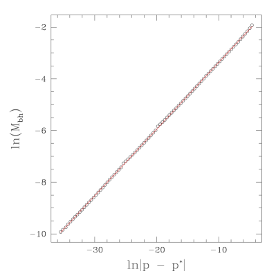
Figure 1: Plot of the observed mass scaling near criticality for the case of the Gaussian family. The measured scaling exponent is $\gamma=0.258$, with uncertainty in the third digit. As we tune arbitrarily close to the critical parameter, $p^{\star}$, black holes of arbitrarily small masses are formed, indicative of a Type II critical solution. The small irregularities visible in the plot are shown and discussed in more detail in Fig. 2

Figure 2: Plot of the residuals of the data shown in Fig. 1 with respect to the computed linear fit. The absence of regular oscillations indicates that the geometry is not discretely self-similar. There are, however, features in the plot, notably the “spikes”, that can be explained as follows. The matter fields have a discretely self-similar nature, but combine to produce a continuously self-similar geometry. Truncation error effects, combined with the fact that our determination of black hole mass is not precise, result in a residual imprint of the DSS nature of the Dirac fields in the plot. In fact the spikes in this plot occur as the amplitude of the Dirac fields reach an extremum near the black hole, periodically in $\ln|p-p^{\star}|$.

IV Self-Similar Ansatz

Given the numerical evidence suggesting the existence of a self-similar solution at the black hole threshold, we proceed to an ab initio computation of the critical solution based on the application of a self-similar ansatz to our system. The development here closely parallels the work done by Hirschmann and Eardley Hirschmann and Eardley (1995), who considered the case of a massless, complex scalar field.

By definition, a self-similar spacetime has a homothetic Killing vector, $\xi$, that obeys

$$\mathcal{L}_{\xi}g_{\mu\nu}=2g_{\mu\nu}$$ (58)

where the factor $2$ is simply a matter of convention. We want to define coordinates, $(\tau,x)$ that are adapted to this self-similar symmetry. Specifically with $\tau$ adapted to the vector field $\xi^{\mu}$, (58) can be written as:

$$\frac{\partial}{\partial\tau}g_{\mu\nu}(\tau,x)=2g_{\mu\nu}(\tau,x).$$ (59)

Performing a separation of variables on the metric tensor and then solving (59) for the $\tau$-dependent part yields

$$g_{\mu\nu}(\tau,x)=e^{2\tau}\tilde{g}_{\mu\nu}(x),$$ (60)

where $\tilde{g}_{\mu\nu}(x)$ is the part of the metric that depends only on $x$. The original coordinates $(t,r)$ are related to $(\tau,x)$ by:

$$\tau=\ln\left|\frac{t^{\star}-t}{L}\right|,\hskip 21.68121ptx=\frac{r}{t^{\star}-t}.$$ (61)

The equations of interest will take the same form for any value of the constant factor, $L$, and without loss of generality, we subsequently take $L=1$. The time $t^{\star}$ is the value of coordinate time to which the self-similar solution asymptotes as it propagates down to arbitrarily small scales, and, from the point of view of critical evolution, is a natural temporal origin for use in describing the dynamics. Further, as mentioned previously, in analyzing self-similar critical solutions, it is natural to adopt a parameterization of the $t$=constant surfaces, such that $t$ coincides with central proper time. We thus adopt such a normalization, and additionally adjust $t$ so that $t^{\star}=0$.

In these new coordinates, the metric (1) becomes

$$ds^{2}=e^{2\tau}\left[(-\alpha(x)^{2}+x^{2}a(x)^{2})d\tau^{2}+2xa(x)^{2}d\tau dx+a(x)^{2}dx^{2}+x^{2}d\theta^{2}+x^{2}\sin^{2}\theta d\phi^{2}\right].$$ (62)

We note that the $\tau$ coordinate is timelike, and, as can be verified by comparing the right hand sides of (60) and (62), that the functions, $\alpha$ and $a$ are functions of the spacelike coordinate, $x$, alone.

In $(\tau,x)$ coordinates, the spinors (42) and (43) become

$$\psi^{+}=\frac{e^{-\tau}}{2\sqrt{\pi}}\frac{e^{i\phi/2}}{x\sqrt{a(x)}}\left(\begin{array}[]{c}F(\tau,x)\sin(\theta/2)\\ G(\tau,x)\cos(\theta/2)\\ F(\tau,x)\sin(\theta/2)\\ G(\tau,x)\cos(\theta/2)\end{array}\right)$$ (63)

$$\psi^{-}=\frac{e^{-\tau}}{2\sqrt{\pi}}\frac{e^{-i\phi/2}}{x\sqrt{a(x)}}\left(\begin{array}[]{c}F(\tau,x)\cos(\theta/2)\\ -G(\tau,x)\sin(\theta/2)\\ F(\tau,x)\cos(\theta/2)\\ -G(\tau,x)\sin(\theta/2)\end{array}\right),$$ (64)

where these expressions were found by transforming the $(t,r)$ parts of (42) and (43) as scalars.

In order to find spinor components that are only functions of $x$, we require knowledge of the $\tau$ dependence of our field quantities. This is determined by performing the coordinate transformations on the equations of motion (44)-(47) and the geometric equations (51) and (53), and then ascertaining what $\tau$ dependence is needed in $F$ and $G$ to produce a set of $\tau$ independent ODEs. A suitable ansatz is

$$F(\tau,x)=e^{\tau/2}e^{i\omega\tau}x(P_{1}(x)+iP_{2}(x))$$ (65)

$$G(\tau,x)=e^{\tau/2}e^{i\omega\tau}x(Q_{1}(x)+iQ_{2}(x)).$$ (66)

where the $\exp(i\omega t)$ terms reflect the fact that, as the PDE solutions have revealed, we expect the matter fields to exhibit discrete self-similarity. Note that $\omega$ as defined here corresponds to $2\pi/\Delta$ (see Hirschmann and Eardley (1995)) where $\Delta$ is the echoing exponent originally defined in Choptuik (1993). Additionally, the extra factor of $x$ is introduced to cast the resulting equations in a more convenient form. Inserting this ansatz into (44)-(47), (51) and (53), we find

$$P_{1}^{\prime}=\frac{1}{x+\alpha/a}\left[-\frac{1}{2}P_{1}-\omega P_{2}-\frac{1}{2}\frac{\alpha}{a}\left(\frac{a^{2}+1}{x}\right)P_{1}+2\alpha P_{1}(P_{1}Q_{1}+P_{2}Q_{2})+\frac{\alpha}{x}Q_{2}\right]$$ (67)

$$P_{2}^{\prime}=\frac{1}{x+\alpha/a}\left[-\frac{1}{2}P_{2}+\omega P_{1}-\frac{1}{2}\frac{\alpha}{a}\left(\frac{a^{2}+1}{x}\right)P_{2}+2\alpha P_{2}(P_{1}Q_{1}+P_{2}Q_{2})-\frac{\alpha}{x}Q_{1}\right]$$ (68)

$$Q_{1}^{\prime}=\frac{1}{x-\alpha/a}\left[-\frac{1}{2}Q_{1}-\omega Q_{2}+\frac{1}{2}\frac{\alpha}{a}\left(\frac{a^{2}+1}{x}\right)Q_{1}-2\alpha Q_{1}(P_{1}Q_{1}+P_{2}Q_{2})+\frac{\alpha}{x}P_{2}\right]$$ (69)

$$Q_{2}^{\prime}=\frac{1}{x-\alpha/a}\left[-\frac{1}{2}Q_{2}+\omega Q_{1}+\frac{1}{2}\frac{\alpha}{a}\left(\frac{a^{2}+1}{x}\right)Q_{2}-2\alpha Q_{2}(P_{1}Q_{1}+P_{2}Q_{2})-\frac{\alpha}{x}P_{1}\right]$$ (70)

$$\frac{a^{\prime}}{a}=\frac{1-a^{2}}{2x}+2x\left(P_{1}P_{2}^{\prime}-P_{1}^{\prime}P_{2}+Q_{1}^{\prime}Q_{2}-Q_{1}Q_{2}^{\prime}\right)+4a\left(P_{1}Q_{1}+P_{2}Q_{2}\right)$$ (71)

$$\frac{\alpha^{\prime}}{\alpha}=\frac{a^{2}-1}{2x}+2x\left(P_{1}P_{2}^{\prime}-P_{1}^{\prime}P_{2}+Q_{1}^{\prime}Q_{2}-Q_{1}Q_{2}^{\prime}\right).$$ (72)

We note that we can cast this system into a canonical form suitable for numerical integration, by using (67)-(70) to eliminate the derivatives of $P$ and $Q$ that appear in the right hand side of the equations for $a$ (71) and $\alpha$ (72).

V Numerical Solution of the Self-Similar ODEs

Having rewritten our equations in a coordinate system adapted to self-similar symmetry, we can now solve the resulting ODEs to determine what we expect will be the CSS critical solution seen at the black hole threshold in the EMD model. Following Hirschmann and Eardley Hirschmann and Eardley (1995), we use a multi-parameter shooting method to integrate the equations subject to regularity and analyticity conditions.

We first observe that the system (67)-(72) has singularities at $x=0$ and at $x=x_{2}=\alpha/a$ (the similarity horizon). Of the infinitely many solutions to the ODEs, we seek one that is analytic at both of these points, as the CSS solution found via solution of the PDEs has this property. Our unknown problem parameters (“shooting” parameters) include the values of some of the fields at the origin, the value of $\omega$ appearing in the ansatz (65)-(66), as well as the value of $x_{2}$ (the position of the similarity horizon). Following Eardley and Hirschmann we shoot outwards from $x=0$ and inwards from $x_{2}=\alpha/a$, comparing solutions at some intermediate point $x_{1}$. This process is automated by starting from some initial guess, then using Newton’s method to determine the shooting parameters for subsequent iterations. In the Newton iteration, we use the square of the differences of the values of the functions and their derivatives at $x_{1}$ (computed from the inwards and outwards integrations) as the goodness-of-fit indicator, which is driven to 0 as the iteration converges.

At $x=0$ we have the following:

$$P_{1}(0)=0$$

$$P_{2}(0)=-Q_{0}$$

$$Q_{1}(0)=Q_{0}$$

$$Q_{2}(0)=0$$

$$\alpha(0)=1$$

$$a(0)=1.$$

Regularity at the origin gives $P_{1}=Q_{2}$ and $P_{2}=-Q_{1}$. We use the global $U(1)$ invariance of our system (67)-(72) to set $P_{1}=0$. This leaves $Q_{0}$ as a shooting parameter.

As noted previously, the location of the similarity horizon (outer boundary of the integration domain) $x_{2}$ is itself a shooting parameter, and is the value $x$ where $\alpha(x)/a(x)=x$. In the limit $x\rightarrow x_{2}$ we have the following:

$$P_{1}(x_{2})=\frac{1}{2a^{2}}\left(-4\alpha Q_{2}^{3}\omega-4\alpha Q_{1}^{2}Q_{2}\omega+2a\omega Q_{1}+Q_{2}a^{3}\right)$$

$$P_{2}(x_{2})=\frac{1}{2a^{2}}\left(4\alpha Q_{1}Q_{2}^{2}\omega+4\alpha Q_{1}^{3}\omega+2a\omega Q_{2}-Q_{1}a^{3}\right)$$

$$Q_{1}(x_{2})=Q_{1}$$

$$Q_{2}(x_{2})=Q_{2}$$

$$\alpha(x_{2})=x_{2}a$$

$$a(x_{2})=a.$$

The shooting parameters at the outer boundary are: $x_{2}$, $Q_{1}(x_{2})$, $Q_{2}(x_{2})$, and $a(x_{2})$. The final shooting parameter is the frequency, $\omega$, for a total of six undetermined parameters.

We find an approximate solution given by

$$x_{2}=5.6740230\pm 0.0000004$$

$$\omega=4.698839\pm 0.000001$$

$$Q_{1}(0)=0.747912623\pm 0.000000006$$

$$Q_{1}(x_{2})=0.00151341532\pm 0.00000000007$$

$$Q_{2}(x_{2})=0.01103266083\pm 0.00000000005$$

$$a(x_{2})=1.1183631604\pm 0.0000000009.$$

where the quoted uncertainty was estimated by solving the system for many different values of $x_{1}$ and observing the changes in the shooting parameters.

VI Comparison of PDE/ODE Solutions

In this section we compare the solution computed from the self-similar ansatz, as just described, to the near-critical solutions calculated from the full PDEs in the $(t,r)$ coordinate system. The ODE solution is the theoretically predicted self-similar solution while the PDE solution can be thought of as collected data. For this comparison, we used data from the Gaussian family. The idea is to treat the ODE solution as the model function and fit it to the PDE data. We perform the fit “simultaneously” at all times by working with the functions as $2$-dimensional solution surfaces in $t$ and $r$. This process is automated by starting from some initial guess for the fitting parameters, then using Newton’s method to determine these parameters for subsequent iterations. In the Newton iteration, we use the least squares of the two solutions:

$$\sum^{N}_{j=1}\left(u^{ODE}_{j}-u^{PDE}_{j}\right)^{2}$$ (73)

as the goodness-of-fit indicator, which is driven towards 0 as the iteration converges. When this happens, we compute the $l_{2}$-norm of the difference of the two solutions:

$$||u||_{2}=\left(\frac{1}{N}\sum^{N}_{j=1}\left(u^{ODE}_{j}-u^{PDE}_{j}\right)^{2}\right)^{1/2}$$ (74)

as an error estimate. In computing both the least squares and the $l_{2}$-norm, the solution to the ODEs and the solution to the PDEs are treated as $N$-element vectors where $N$ is the total number of grid points on the $2$-dimensional grid in $t$ and $r$.

For the case of $a(t,r)$, we use $t^{\star}$ as the fitting parameter. Once $t^{\star}$ is found, the $l_{2}$-norm of the difference of the two solutions is $0.00159$. We display the results of this fitting process as a sequence of snapshots in time in Fig. 3.

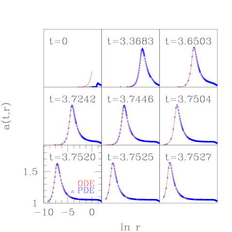
Figure 3: Evolution of the metric variable, $a(t,r)$, for a slightly supercritical evolution, overlayed with the solution to the ODEs. The frames are output logarithmically in central proper time, as measured from $t^{\star}$. The function’s peak reaches a value of approximately $1.6$ and remains there as the solution continuously repeats itself on ever smaller scales.

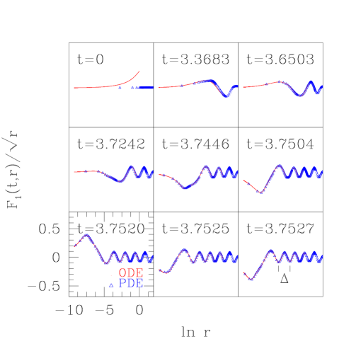
Figure 4: Comparison of $F_{1}(t,r)$ for a slightly supercritical PDE evolution with the solution found from the self-similar ansatz. As in Fig. 3, the frames are output logarithmically in central proper time, measured from $t^{\star}$. The function oscillates and discretely repeats itself on smaller and smaller scales. The particular combination of $F_{1}(t,r)/\sqrt{r}$ is the natural scaling variable as can be deduced by noting that the Dirac fields have units of $($Length$)^{1/2}$, and as shown explicitly by the $\tau$ dependence of (65) and (66). The echoing exponent, $\Delta$, calculated via $\Delta=2\pi/\omega$, where $\omega$ is computed from the ODE solution, is also shown.

Comparing the Dirac fields is a little more involved since there are a number of unspecified parameters and phases that must be determined. From the ansatz (65)-(66) we have:

$$F_{1}(t,r)=\frac{rA_{1}}{(t^{\star}-t)^{\frac{1}{2}}}\left[P_{1}(t,r)\cos(\omega\ln(t^{\star}-t)+\phi_{1})-P_{2}(t,r)\sin(\omega\ln(t^{\star}-t)+\phi_{1})\right]$$

$$F_{2}(t,r)=\frac{rA_{2}}{(t^{\star}-t)^{\frac{1}{2}}}\left[P_{1}(t,r)\sin(\omega\ln(t^{\star}-t)+\phi_{2})+P_{2}(t,r)\cos(\omega\ln(t^{\star}-t)+\phi_{2})\right]$$

$$G_{1}(t,r)=\frac{rA_{2}}{(t^{\star}-t)^{\frac{1}{2}}}\left[Q_{1}(t,r)\cos(\omega\ln(t^{\star}-t)+\phi_{2})-Q_{2}(t,r)\sin(\omega\ln(t^{\star}-t)+\phi_{2})\right]$$

$$G_{2}(t,r)=\frac{rA_{1}}{(t^{\star}-t)^{\frac{1}{2}}}\left[Q_{1}(t,r)\sin(\omega\ln(t^{\star}-t)+\phi_{1})+Q_{2}(t,r)\cos(\omega\ln(t^{\star}-t)+\phi_{1})\right].$$ (75)

We note that $F_{1}$ and $G_{2}$ have the same phase, $\phi_{1}$, while the pair $F_{2}$ and $G_{1}$ have the same phase $\phi_{2}$. This is expected from the coupling of (44)-(47). The equations of motion may be invariant under changes of these phases, but (51) and (53) are not. In order to have the entire system be invariant under changes in the phases, we must have:

$$A_{1}A_{2}=\frac{1}{\cos(\phi_{1}-\phi_{2})}$$

We see that the amplitudes of the fields must change only if the relative phase, $\phi_{1}-\phi_{2}$, changes. We merely note this fact for completeness but do not use it to reduce the number of fit parameters.

The comparison of the fields as found from the PDEs and ODEs is carried out in much the same way as it is done for the metric variable, $a(t,r)$. The goodness-of-fit is again defined to be the least squares of the two solutions but this time, the parameter $t^{\star}$ is kept fixed and the phase $\phi_{j}$ and amplitude $A_{j}$ are used as fitting parameters ($j=1,2)$. The $l_{2}$-norm of the difference of the solutions for $F_{1}$ is $0.000195$. The $l_{2}$-norm of the difference of the solutions for $G_{1}$ is $0.00024$. Fig. 4 illustrates the results of this comparison of the ODE and PDE solutions for $F_{1}$.

VII Conclusions

We have investigated the spherically symmetric Einstein-massless-Dirac system at the threshold of black hole formation. We have found strong evidence for a Type II critical solution, and an associated mass scaling law with a universal exponent $\gamma\sim 0.26$. The solution exhibits continuous self-similarity in the geometric variables and discrete self-similarity in the components of the Dirac fields, the latter characterized by an echoing exponent $\Delta\sim 1.34$. Using a self-similar ansatz, we then reduced the equations of motion governing the model to a set of ODEs whose solution, given appropriate regularity conditions, is in very good agreement with the critical solution obtained from the original PDEs.