Brane classical and quantum cosmology from an effective action

Abstract

Motivated by the Randall-Sundrum brane-world scenario, we discuss the classical and quantum dynamics of a $(d+1)$-dimensional boundary wall between a pair of $(d+2)$-dimensional topological Schwarzschild-AdS black holes. We assume there are quite general — but not completely arbitrary — matter fields living on the boundary “brane universe” and its geometry is that of an Friedmann-Lemaître-Robertson-Walker (FLRW) model. The effective action governing the model in the mini-superspace approximation is derived. We find that the presence of black hole horizons in the bulk gives rise to a complex action for certain classically allowed brane configurations, but that the imaginary contribution plays no role in the equations of motion. Classical and instanton brane trajectories are examined in general and for special cases, and we find a subset of configuration space that is not allowed at the classical or semi-classical level; these correspond to spacelike branes carrying tachyonic matter. The Hamiltonization and Dirac quantization of the model is then performed for the general case; the latter involves the manipulation of the Hamiltonian constraint before it is transformed into an operator that annihilates physical state vectors. The ensuing covariant Wheeler-DeWitt equation is examined at the semi-classical level, and we consider the possible localization of the brane universe’s wavefunction away from the cosmological singularity. This is easier to achieve for branes with low density and/or spherical spatial sections.

I Introduction

The idea that our universe might be a 4-dimensional hypersurface embedded in a higher-dimensional manifold is an old one with a long history, as well as the subject of a considerable amount of contemporary interest. The primordial impetus for this line of study comes from the work of Kaluza Kaluza (1921), who showed that one can obtain a classical unification of gravity and electromagnetism by adding an extra dimension to spacetime (1921); and Klein Klein (1926), who suggested that extra dimensions have a circular topology of very small radius and are hence unobservable (1926). The latter idea, the so-called “compactification” paradigm, came to dominate most approaches to higher-dimensional physics, the most notable of which was early superstring theory. However, a number of papers have appeared in the intervening years that do not assume extra dimensions with compact topologies; early examples include the works of Joseph Joseph (1962), Akama Akama (1982), Rubakov & Shaposhnikov Rubakov and Shaposhnikov (1983), Visser Visser (1985), Gibbons & Wiltshire Gibbons and Wiltshire (1987), and Antoniadis Antoniadis (1990). A systematic and independent approach to the 5-dimensional, non-compact Kaluza-Klein scenario, known as Space-Time-Matter (STM) theory, followed Wesson and Ponce de Leon (1992); Wesson et al. (1996); Overduin and Wesson (1997); Wesson (1999). Then, in 1996 Horava & Witten showed that the compactification paradigm was not a prerequisite of string theory with their discovery of an 11-dimensional theory on the orbifold $\mathbb{R}^{10}\times S^{1}/\mathbb{Z}_{2}$, which is related to the 10-dimensional $E_{8}\times E_{8}$ heterotic string via dualities Horava and Witten (1996). In this theory, standard model interactions are confined to a lower-dimensional hypersurface, known as a “brane”, on which the endpoints of open strings reside, while gravitation propagates in the higher-dimensional bulk. This situation has come to be known as the “braneworld scenario.” The works of Arkani-Hamed et al. Arkani-Hamed et al. (1998); Antoniadis et al. (1998); Arkani-Hamed et al. (1999) and Randall & Sundrum (RS) Randall and Sundrum (1999a, b), which used non-compact extra dimensions to address the hierarchy problem of particle physics and demonstrated that the graviton ground state can be localized on a 3-brane in 5 dimensions, won a large following for the braneworld scenario and a virtual flood of papers dealing with non-compact, higher-dimensional models of the universe soon followed.

One particular type of braneworld model that has received much attention concerns the idea that the universe could be a 4-dimensional boundary wall between a pair of 5-dimensional Schwarzschild-anti deSitter (S-AdS₅) or Riesner-Nordström-anti deSitter black holes. The Friedman equation governing the classical dynamics of such a scenario has been derived using Israel’s junction conditions Israel (1966) for arbitrary brane matter-content Kraus (1999); Barcelo and Visser (2000), and for the case where the only matter energy on the brane is from its tension or vacuum energy Savonije and Verlinde (2001); Nojiri et al. (2002); Gregory and Padilla (2002a). There have been numerous studies of the classical brane trajectories associated with such scenarios that have found that the “brane universe” can exhibit non-standard bouncing or cyclic behaviour Campos and Sopuerta (2001); Myung (2003); Mukherji and Peloso (2002); Medved (2002). Generalizations to six-dimensional bulks have also been considered Cuadros-Melgar (2003).

The natural extension of this work is the problem of quantizing these braneworld models. Several authors have found it useful to appeal to the well-known 4-dimensional formalism of quantum cosmology to initiate studies of this issue, particularly concerning the “quantum birth” of the universe Vilenkin (1982); Hartle and Hawking (1983); Vilenkin (1984); Linde (1984); Vilenkin (1986); Rubakov (1984). The advantage of the quantum cosmology approach are obvious: the mini-superspace approximation allows one to pick a few of the system’s degrees of freedom to treat quantum mechanically while the others are represented by their classical solutions. However, there are a number of well-catalogued problems associated with quantum cosmology; including the problem of time Kuchar̆ (1991), the validity of the mini-superspace approximation, and the problem of assigning appropriate boundary conditions to the wavefunction of the universe Hartle (1997).

Despite these difficulties, the canonical quantum cosmology for the vacuum branes surrounding bulk black holes has been considered from the point of view of an effective action Koyama and Soda (2000); Biswas et al. (2003), while the problem for a vacuum brane bounding pure AdS space has also been dealt with Anchordoqui et al. (2000). The case where there is some conformal field theory living on the brane has also been considered for various bulk manifolds Nojiri et al. (2000); Nojiri and Odintsov (2000, 2001). Related to these studies are works that consider the quantum creation (or decay) of brane universes via saddle-point approximations to path integrals Gorsky and Selivanov (2000); Ida et al. (2002); Gregory and Padilla (2002b) — often in bulk manifolds other than S-AdS₅ — as well as papers that consider the classical and quantum dynamics of “geodetic brane universes” Karasik and Davidson (2002); Cordero and Vilenkin (2002); Cordero and Rojas (2003).

It should be mentioned that quantum brane world models where the bulk is sourced by black holes are related to 4-dimensional problems other than canonical quantum cosmology. Indeed, they share many of the same features as the problem of the quantum collapse of spherical matter shells, which has been rather whimsically named “quantum conchology” by some authors Hajicek (1992); Hajicek et al. (1992); Friedman et al. (1997); Hajicek and Bicak (1997); Kuchar (1999); Corichi et al. (2002); Hajicek (2002). Also, the problem associated with the quantum birth of a braneworld sandwiched in between topological bulk black holes is almost the inverse of the problem of the creation of 4-dimensional topological black holes separated by a 3-dimensional domain wall Mann and Ross (1995); Caldwell et al. (1996); Mann (1998).

The purpose of this paper is to analyze the classical and quantum mechanics of a $d$-brane acting as a boundary between a pair of “topological” S-AdS_(d+2) black holes from the point of view of an effective action. The treatment is designed to be as self-contained and transparent as possible. The action for our model in the mini-superspace approximation is explicitly constructed from the standard action of general relativity in Sec. II. One of the novel features of our analysis is that we allow for arbitrary matter living on the brane, provided that the perfect cosmological principle (PCP) is obeyed. The true dynamical variables in our action are the brane radius and the matter field configuration variables. We also retain a gauge degree of freedom in the form of the lapse function on the brane, which is associated with transformations of the $(d+1)$-dimensional time coordinate. As a result, our effective action is reparametrization invariant. Another way in which our work differs from previous efforts is that we pay special attention to the behavior of the action as the brane crosses the bulk black hole horizon — if such a horizon exists — and we will demonstrate that even though the brane trajectory is perfectly well behaved at the horizon, the action becomes complex valued. This behaviour is reminiscent of the action governing the collapse of thin matter shells in 4 dimensions. We argue that a complex action can be partly avoided by the addition of total time derivatives to the Lagrangian in certain classically allowed parts of configuration space — which is the manifold spanned by the system’s coordinates and velocities — resulting in an piecewise-defined action. However, we do find a portion of configuration space where it is impossible to make the action real. When the brane is within this region, its normal becomes timelike and comoving brane observers follow spacelike paths. Hence we name this portion of configuration space the “tachyon region”.

Sec. III is devoted to the classical cosmology of our model as derived from direct variation of the effective action. We analyze the Friedman equation in the general situation and determine the criterion for classically allowed and classically forbidden regions. We also derive the Newtonian limit of the brane’s equation of motion and show that it is nothing more than an energy conservation equation for a thin-shell encircling a central mass with zero total energy. We then turn our attention to a special case that is suitable for exact analysis. In that case, the bulk cosmological constant is set to zero and the spatial sections of the brane are flat, while the matter on the brane takes the form of the brane tension and a cosmological dust fluid. We demonstrate that the solutions of the Friedman equation exhibit exotic bounce and crunch behaviour for negative mass bulk black holes; i.e., one does not need a charged bulk black hole to avoid the cosmological singularity. However, at least for this special case, one must allow the energy conditions to be violated in the bulk. We also look for classical brane trajectories that transverse the tachyon region and find that only possibility is to allow the brane’s density to be imaginary. This is not surprising; recall that only point particles with imaginary mass can travel on spacelike trajectories.

The Hamiltonization and quantization of the model is the subject of Sec. IV. In order to maintain a certain level of rigor, we find that the reparametrization invariance of the action and the general nature of the matter fields demand an extended foray into Dirac’s formalism dealing with the Hamiltonian mechanics of constrained systems Dirac (1964); Gitman and Tyutin (1990). The piecewise nature of the action comes back to haunt us here; in order to avoid the consideration of a complex phase space, we find that it is necessary to define canonical momenta and constraints in a piecewise fashion. Continuity of the latter across the horizon is resolved by rewriting the first-class Hamiltonian constraint in an algebraically equivalent form and by making minimal assumptions about the matter fields. We ultimately obtain a continuous set of first-class constraints and Dirac bracket structure suitable for Dirac quantization. The transformation of the Hamiltonian constraint represents a significant departure from previous studies Anchordoqui et al. (2000); Biswas et al. (2003), which is another “twist” that has a number of beneficial qualities. The Wheeler-DeWitt equation obtained upon quantization is shown to be equivalent to a $(d+2)$-dimensional covariant wave equation — which means that it ought to be invariant under $(d+2)$-dimensional coordinate transformations — and reduces to a one-dimensional Schrödinger equation that exhibits no pathological behaviour at the position of the bulk horizon; this is in contrast to the wave equation derived in Biswas et al. (2003). We then specialize to the case where the brane matter consists of vacuum energy plus dust, and demonstrate that for certain model parameters the wavefunction of the universe can be localized away from the cosmological singularity by potential barriers in the Wheeler-DeWitt equation. The degree of localization is characterized by the WKB tunnelling amplitude through those same barriers, which is calculated explicitly for certain model parameters. We find that singularity avoidance is more likely for branes with low matter density and spherical spatial sections.

Finally Sec. V gives a summary of our results and suggestions for future projects based on this work, of which there are several.

II An effective action for the brane world

The model that we will be concerned with in this paper is as follows: Consider a $d$-brane $\Sigma$ that acts as a domain wall between two bulk $N$-dimensional manifolds, where $N=d+2$. We treat the embedding functions of the brane as the dynamical degrees of freedom of the model, but we regard the components of the two bulk metrics as fixed; i.e, we are considering a brane propagating in a static background. The other dynamical degrees of freedom in the model come from matter fields living on $\Sigma$, about which we will make minimal assumptions.

The structure of the brane is taken to be that of an $(d+1)$-dimensional FLRW model; i.e., $\Sigma=\mathbb{R}\times{\mathbb{S}}_{d}^{(k)}$, where ${\mathbb{S}}_{d}^{(k)}$ is an $d$-dimensional Euclidean space of constant curvature $k=-1,0,1$. We take $\theta=\{\theta^{1},\ldots,\theta^{d}\}$ to be a suitable coordinate system on ${\mathbb{S}}_{d}^{(k)}$ such that the metric is $\sigma^{(k,d)}_{ab}$, where $a,b=1\ldots d$. A necessary assumption for a well defined action of our model is that ${\mathbb{S}}_{d}^{(k)}$ is globally compact; i.e., if $k=0$ we take ${\mathbb{S}}_{d}^{(k)}$ to be an $d$-torus and if $k=-1$ we take ${\mathbb{S}}_{d}^{(k)}$ to be a compact $d$-hyperboloid. The finite $d$-dimensional volume of the unit radius submanifold ${\mathbb{S}}_{d}^{(k)}$ is then given by

$${\mathcal{V}}^{(k)}_{d}=\oint\limits_{{\mathbb{S}}_{d}^{(k)}}d^{d}\theta\,\sqrt{\sigma^{(k,d)}},$$ (1)

where $\sigma^{(k,d)}=\det\sigma^{(k,d)}_{ab}$. Our work will not depend on the actual value of ${\mathcal{V}}^{(k)}_{d}$ — other than the fact that it is finite — so we do not need to specify the periodicity of the $\theta^{a}$ coordinates in the $k=0$ or $-1$ cases (when $k=1$ we take $\theta^{a}$ to be the standard angular coordinates on an $d$-sphere).

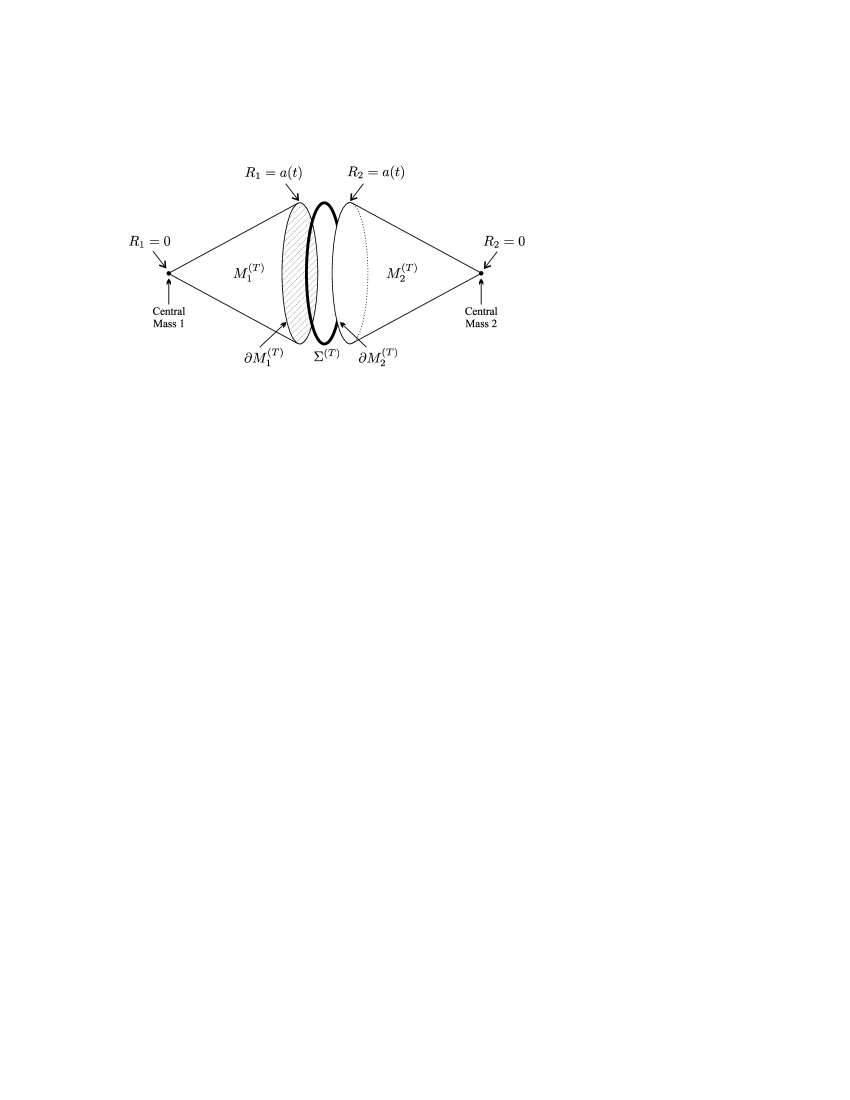
Figure 1: A pictorial representation of a spatial slice of our model. The $(T)$ superscripts are meant to convey that we are showing the $T=$ constant surfaces of the relevant manifolds. We have suppressed $d-1$ dimensions on the ${\mathbb{S}}_{d}^{(k)}$ submanifolds so that they appear as vertical circles and $M_{1,2}^{(T)}$ appear as 2-surfaces. The finite amount of space between $\partial M_{1}^{(T)}$, $\Sigma^{(T)}$, and $\partial M_{2}^{(T)}$ is included to ease with visualization; in actuality those three $d$-surfaces are coincident. Note that the spatial slice is compact for finite $a(t)$ and that each of the bulk regions has a distinct boundary.

The brane $\Sigma$ is sandwiched between two $N$-dimensional bulk spaces $M_{1}$ and $M_{2}$, as shown in Fig. 1. We impose $\mathbb{Z}_{2}$ symmetry across the brane, which implies that $M_{1}$ and $M_{2}$ are “mirror images” of one another. Each of the bulk spaces is identified with a topological S-AdS_N manifold. On each side of the brane, we place a bulk coordinate system $x_{(1,2)}=\{T,\theta^{1},\ldots,\theta^{d},R_{1,2}\}$ such that the metric $g^{(1,2)}_{AB}$ on $M_{1,2}$ is

$$ds^{2}_{(1,2)}=-F(R_{1,2})\,dT^{2}+\frac{dR_{1,2}^{2}}{F(R_{1,2})}+R_{1,2}^{2}\sigma^{(k,d)}_{ab}d\theta^{a}d\theta^{b},$$ (2)

where $A,B=0\ldots(d+1)$. This reduces to the usual Schwarzschild-AdS line element if we set $k=1$ and is a solution of the bulk Einstein field equations

$$G^{(1,2)}_{AB}=\Lambda g^{(1,2)}_{AB}$$ (3)

if we set

$$F(R)=k-\frac{K}{R^{d-1}}+\frac{2\Lambda R^{2}}{d(d+1)}.$$ (4)

The constant $K$ is linearly proportional to the ADM mass of the central object in each of the bulk regions:

$$K=\frac{2MG_{N}}{d-1}\frac{\Omega_{d}}{{\mathcal{V}}^{(k)}_{d}},$$ (5)

where $\Omega_{d}\equiv{\mathcal{V}}^{(+)}_{d}$ and we define the $N$-dimensional Newton’s constant by

$$\kappa_{N}^{2}=\left(\frac{N-2}{N-3}\right)\Omega_{N-2}G_{N}=\left(\frac{d}{d-1}\right)\Omega_{d}G_{d+2},$$ (6)

where $\kappa_{N}^{2}$ is the higher-dimensional gravity matter coupling in Einstein’s equations. We note that (2) solves (3) even if $K$ is negative. In this paper, we will generally restrict ourselves to $\Lambda\geq 0$ — i.e., AdS space — although this is not a critical assumption for any of the derivation.

We should comment on the horizon structure of the bulk manifolds. In general, there will be a Killing horizon at any $R=R_{H}$ such that $F(R_{H})=0$. For the moment, let us focus in on the most physically relevant case of $d=3$. Then we find the following solution for $R_{H}$:

$$R_{H}^{2}=\begin{cases}\sqrt{\frac{6K}{\Lambda}},&k=0,\\ -\frac{3k}{\Lambda}\left(-1\pm\sqrt{1+\frac{2}{3}\Lambda K}\right),&k=\pm 1.\end{cases}$$ (7)

For $K>0$, it is easy to see that there is only one real and positive solution for $R_{H}$ for all values of $k$. When $K<0$, there is no horizon for the $k=0$ and $k=+1$ case. However, if $\Lambda|K|<\tfrac{3}{2}$, there will be two positive and real solutions for $R_{H}$ in the $k=-1$ case. As long as $\Lambda>0$, $F(a)\rightarrow\infty$ when $a\rightarrow\infty$. This prompts us to use the terminology that “outside the horizon” refers to regions with $F(a)>0$ and that “inside the horizon” refers to regions with $F(a)<0$. Clearly the labels are not strictly applicable to the $k=-1$ case and might not sense when $d>3$ or $\Lambda=0$. However, we do find it useful to apply these terms to the general situation and with the preceding caveat we forge ahead.

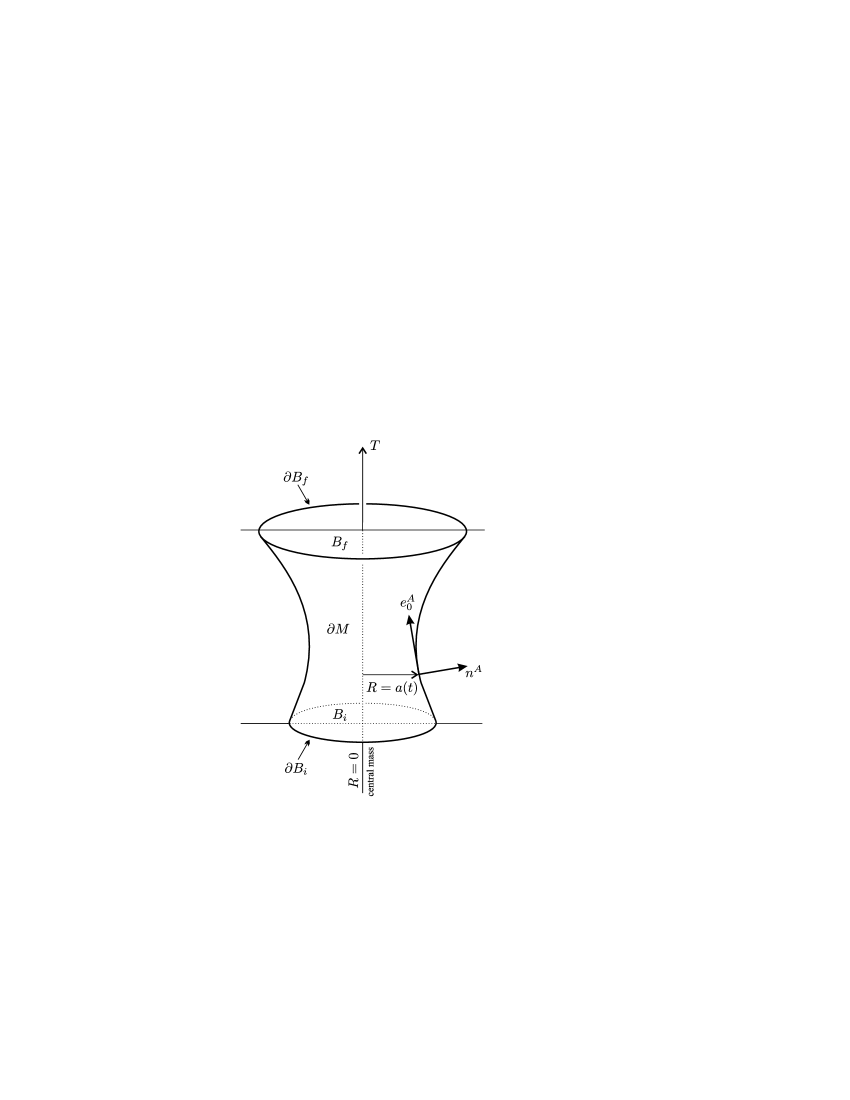
Figure 2: A pictorial representation of one of the bulk sections of our model. As if Fig. 1, we suppress $d-1$ dimensions on ${\mathbb{S}}_{d}^{(k)}$ to obtain a 3-dimensional picture. The bulk $M$ is the region bounded by $\partial M\cup B_{i}\cup B_{f}$.

We now return to the case of arbitrary $d$. The structure of each bulk section is shown in Fig. 2. The boundary of $M_{1,2}$ is given by $\partial M_{1,2}\cup B_{i}\cup B_{f}$. The $B_{i}$ and $B_{f}$ hypersurfaces are defined by $T=T_{i}$ and $T_{f}$ respectively, and will represent the endpoints of temporal integrations in the action for our model. The other boundary $\partial M_{1,2}$ is described by the hypersurface

$$R_{1,2}=a(t),\quad T={T}(t).$$ (8)

Here, $t$ is a parameter. In principle, we can identify $M_{1,2}$ with the portion of the Schwarzschild-AdS manifold interior or exterior to the $\partial M_{1,2}$ world-tube. However, we want the spatial sections of our model to be compact, so we take $M_{1,2}$ to be the $(d+2)$-manifold inside $\partial M_{1,2}$. Let us define a function $\Phi(t)\in\mathbb{R}^{+}$ as

$$\Phi^{2}\equiv F(a)\dot{T}^{2}-\frac{1}{F(a)}\dot{a}^{2},$$ (9)

where an overdot stands for $d/dt$. With this definition, we see that the induced metric on $\partial M_{1}$ is identical to that of $\partial M_{2}$ and is given by

$$ds_{\Sigma}^{2}=-\Phi^{2}(t)\,dt^{2}+a^{2}(t)\sigma^{(k,d)}_{ab}d\theta^{a}d\theta^{b}.$$ (10)

We identify this with the metric $h_{\alpha\beta}$ on the brane in the $y=\{t,\theta^{1},\ldots,\theta^{d}\}$ coordinate system, where $\alpha,\beta=0\ldots d$. All three of the $(d+1)$-surfaces $\partial M_{1,2}$ and $\Sigma$ are bounded by $\partial B_{i}$ and $\partial B_{f}$, which can be thought of as $t=t_{i}$ and $t_{f}$ $d$-surfaces respectively. The intrinsic geometry of the brane is hence specified by the two functions $a(t)$ and $\Phi(t)$, which we take to be the brane’s generalized coordinate degrees of freedom. However, it is obvious that the lapse function $\Phi(t)$ does not represent a genuine physical degree of freedom because it can be removed from the discussion via a reparametrization of the brane’s time coordinate $t$. It is therefore a gauge degree of freedom whose existence implies that there are first class constraints in our system Dirac (1964). This is important in what follows.

The last ingredient of the model is the matter fields living on $\Sigma$. We will characterize the matter degrees of freedom by the set of “coordinates” $\psi=\{\psi_{i}\}$. Here, $\psi$ can include scalar or spinorial fields, perfect fluid velocity potentials Schutz (1970b), or other types of fields. At this stage, the only real restriction we place on $\psi$ comes from the fact that our assumed form of the brane metric is isotropic and homogeneous, and hence obeys the perfect cosmological principle (PCP). This means that $\psi$ can only depend on $t$ and not $\theta^{a}$. We will need the matter Lagrangian density, which in keeping with the PCP must be of the form

$${\mathcal{L}}_{m}={\mathcal{L}}_{m}\left(\psi,\dot{\psi};a,\Phi\right).$$ (11)

Notice that ${\mathcal{L}}_{m}$ is independent of derivatives of the induced metric, which is a common and non-restrictive assumption. Later, we will need the stress energy tensor associated with the matter fields, which is given by

$$T_{\alpha\beta}=-2\frac{\delta{\mathcal{L}}_{m}}{\delta h^{\alpha\beta}}+{\mathcal{L}}_{m}h_{\alpha\beta}.$$ (12)

We are now in position to calculate the action of our model. It is composed of five parts as follows Karasik and Davidson (2002):

$$S=\frac{1}{\mathcal{N}}[S(M_{1})+S(\partial M_{1})+S(\Sigma)+S(\partial M_{2})+S(M_{2})],$$ (13)

where ${\mathcal{N}}$ is a normalization constant that will be selected later, and

$$S(M_{1,2}) = \int\limits_{M_{1,2}}d^{d+2}x_{(1,2)}\sqrt{-g^{(1,2)}}\,\left[{\mathcal{R}}^{(1,2)}+2\Lambda\right],$$ (14a)

$$S(\partial M_{1,2}) = 2\int\limits_{\partial M_{1,2}}d^{d+1}y\sqrt{-h}\,\text{Tr}\left[{\mathcal{K}}^{(1,2)}\right],$$ (14b)

$$S(\Sigma) = 2\kappa^{2}_{N}\int\limits_{\Sigma}d^{d+1}y\sqrt{-h}\,{\mathcal{L}}_{m}.$$ (14c)

In these expressions, ${\mathcal{R}}^{(1,2)}$ is the Ricci scalar in the bulk regions, $\text{Tr}\left[{\mathcal{K}}^{(1,2)}\right]$ is the trace of the extrinsic curvature of $\partial M_{1,2}$. There is no contribution to the action from the spacelike boundaries $B_{i}$ and $B_{f}$ of $M_{1,2}$ because those surfaces have vanishing extrinsic curvature. The $\mathbb{Z}_{2}$ symmetry immediately gives us

$$S(M_{1})=S(M_{2})\equiv S(M).$$ (15)

Now, what does this symmetry imply for the boundary terms? Note that $\text{Tr}\left[{\mathcal{K}}^{(1,2)}\right]$ is calculated with the outward-pointing normal vector field, which means that the normal on $\partial M_{1}$ is anti-parallel to the normal on $\partial M_{2}$. Usually, the $\mathbb{Z}_{2}$ symmetry gives that the sign of the extrinsic curvature is inverted as one traverses the brane, but that assumes a continuous normal vector. In our situation, we expect $\text{Tr}\left[{\mathcal{K}}^{(1)}\right]=\text{Tr}\left[{\mathcal{K}}^{(2)}\right]$, which yields

$$S(\partial M_{1})=S(\partial M_{2})\equiv S(\partial M).$$ (16)

Hence, we only have to calculate three separate quantities to arrive at the total action.

The actual calculation of $S$ is straightforward but lengthy, involving partial integrations, the elimination non-dynamical contributions, and integrating over the bulk manifolds and spatial directions on the brane; full details can be found in refs. Seahra et al. (2003); Seahra (2003). The final result is

$$S=\int_{t_{i}}^{t_{f}}dt\,\Phi a^{d-1}\left\{-\frac{\dot{a}}{\Phi}\mathrm{arcsinh}\left[\frac{\dot{a}}{\Phi\sqrt{F(a)}}\right]+\sqrt{\frac{\dot{a}^{2}}{\Phi^{2}}+F(a)}+a\alpha_{m}{\mathcal{L}}_{m}\right\},$$ (17)

where we have made the choices

$${\mathcal{N}}\equiv 4d{\mathcal{V}}^{(k)}_{d},\quad\alpha_{m}\equiv\frac{\kappa_{N}^{2}}{2d}.$$ (18)

This is the effective action for our model. The degrees of freedom are the brane radius $a(t)$, the lapse function $\Phi(t)$, and the matter coordinates $\psi_{i}(t)$. We note that under an arbitrary reparametrization of the time

$$t\rightarrow\tilde{t}=\tilde{t}(t),$$ (19)

the lapse transforms as

$$\Phi\rightarrow\tilde{\Phi}=\Phi\frac{dt}{d\tilde{t}}.$$ (20)

Assuming that the matter Lagrangian is a proper relativistic scalar, we see that the total action is invariant under time transformations. Systems with this property have Hamiltonian functions that are formally equal to constraints and hence vanish on solutions, which is what we will see explicitly in Sec. IV. The fact that our action involves constraints should not be surprising because we have already identified $\Phi$ as a gauge degree of freedom. Also, the zero Hamiltonian phenomena is a trademark of fully covariant theory such as general relativity.

Before leaving this section, we note that our action can become imaginary for certain values of $(a,\dot{a})$; i.e., when $F(a)<0$. To get around a complex action, we consider the following identities:

$$\ln(i) = \mathrm{arcsinh}(iz)-\mathrm{arccosh}(z),$$ (21a)

$$\ln(-1) = \mathrm{arccosh}(z)+\mathrm{arccosh}(-z).$$ (21b)

There are a couple of subtle points that one must remember when working with these complex identities. The first is that we must specify a branch cut in order to evaluate the logarithms of complex quantities. In all cases, we assume that the argument of complex numbers lies in the interval $(-\pi,\pi]$ so that $\ln(i)=i\pi/2$ and $\ln(-1)=i\pi$. This cut also makes the square root function single-valued on the negative real axis; we have that $\sqrt{-x}=i\sqrt{x}$ for all $x\in\mathbb{R}^{+}$. The other issue is the fact that the arccosh function is multi-valued on the positive real axis. We will always take the principle branch, with $x\in[1,\infty)$ implying that $\mathrm{arccosh}(x)>0$.

Having clarified our choices for the structure of the complex plane, let us now define a pair of alternative actions $S_{\pm}$ by

$$S_{\pm}=\int_{t_{i}}^{t_{f}}dt\,\Phi a^{d-1}\left\{\mp\frac{\dot{a}}{\Phi}\mathrm{arccosh}\left[\frac{\pm\dot{a}}{\Phi\sqrt{-F(a)}}\right]+\sqrt{\frac{\dot{a}^{2}}{\Phi^{2}}+F(a)}+a\alpha_{m}{\mathcal{L}}_{m}\right\}.$$ (22)

Using the identity (21a) it is not difficult to show that

$$S-S_{+}=-\frac{\ln(i)}{n}\int_{t_{i}}^{t_{f}}dt\frac{d}{dt}a^{d},$$ (23)

and using (21b) we have

$$S_{+}-S_{-}=-\frac{\ln(-1)}{n}\int_{t_{i}}^{t_{f}}dt\frac{d}{dt}a^{d}.$$ (24)

Therefore, the three actions $S$ and $S_{\pm}$ differ by terms proportional to the integral of total time derivatives. This means that the variations of each are the same, and each one is a valid action for our model. Now, each action will be real and well-behaved for different regions of the $(a,\dot{a})$-plane, which are depicted in Fig. 3 and defined by

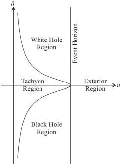
Figure 3: A sketch of the various regions in the position-velocity $(a,\dot{a})$-plane describing our model when the bulk manifold contains an event (Killing) horizon.

Exterior Region $$\equiv \bigg{\{}a\in\mathbb{R}^{+},\,\dot{a}\in\mathbb{R}\,\bigg{|}\,F(a)>0\bigg{\}},$$ (25a)

White Hole Region $$\equiv \left\{a\in\mathbb{R}^{+},\,\dot{a}\in\mathbb{R}\,\bigg{|}\,F(a)<0,\,0<\dot{a},\,0<\frac{\dot{a}^{2}}{\Phi^{2}}+F(a)\right\},$$ (25b)

Black Hole Region $$\equiv \left\{a\in\mathbb{R}^{+},\,\dot{a}\in\mathbb{R}\,\bigg{|}\,F(a)<0,\,\dot{a}<0,\,0<\frac{\dot{a}^{2}}{\Phi^{2}}+F(a)\right\},$$ (25c)

Tachyon Region $$\equiv \left\{a\in\mathbb{R}^{+},\,\dot{a}\in\mathbb{R}\,\bigg{|}\,\frac{\dot{a}^{2}}{\Phi^{2}}+F(a)<0\right\}.$$ (25d)

The original action $S$ is real-valued in the exterior region, while the alternative actions $S_{\pm}$ are well-behaved in the white and black hole regions respectively. The adjectives “White Hole” and “Black Hole” are used because the brane is moving away from the central singularity when it is in the former region and towards the singularity when in the latter. The fourth region is intriguing; when the brane is inside it all of the actions we have written down thus far fail to be real. Also, when inside this region it is impossible to solve equation (9) for $\Phi\in\mathbb{R}$, which means the brane’s “timelike” tangent vector $e^{A}_{0}$ becomes spacelike. Since the brane behaves like a particle with imaginary mass in this portion of the position-velocity plane, we label it as the “Tachyon Region”. What is the form of the action for our model inside the tachyon region? To answer this, we can analytically continue the $S_{\pm}$ actions by using the identities

$$0 = \text{arccosh}(z)-i\,\mathrm{arccos}(z),$$ (26a)

$$\pi = \text{arccos}(x)+\text{arccos}(-x).$$ (26b)

When the first of these is applied to the $S_{\pm}$ actions, we obtain two distinct expressions. But if we apply the second identity to the action derived from $S_{-}$ and discard a boundary term, we arrive at the tachyon action:

$$S_{\mathrm{tach}}=i\int_{t_{i}}^{t_{f}}dt\,\Phi a^{d-1}\left\{-\frac{\dot{a}}{\Phi}\mathrm{arccos}\left[\frac{\dot{a}}{\Phi\sqrt{-F(a)}}\right]+\sqrt{-\left[\frac{\dot{a}^{2}}{\Phi^{2}}+F(a)\right]}-ia\alpha_{m}{\mathcal{L}}_{m}\right\}.$$ (27)

This action is valid throughout the tachyon region, and is explicitly complex-valued. Recall that when the action for a mechanical system is complex when evaluated along a given trajectory that solves the equation of motion, that trajectory is considered to be classically forbidden. In our case, this means that the tachyon region is inaccessible by the brane in the context of classical mechanics. We will revisit this notion in the context of semi-classical considerations shortly.

To summarize, we have obtained the reduced action(s) governing the motion of the brane in our model. The degrees of freedom are the brane radius, the lapse function, and whatever coordinates we need to describe the matter living on the brane. When there are horizons in the bulk, the $(a,\dot{a})$-plane acquires the structure depicted in Fig. 3. We find that four actions are needed in this case: $S$, $S_{\pm}$, and $S_{\mathrm{tach}}$. These actions differ by integrals of time derivatives, and are hence equivalent.

III The dynamics of the classical cosmology

III.1 The Friedman equation exterior to the tachyon region

We now turn our attention to the classical dynamics of our system. The equation of motion that we will be primarily concerned with can be obtained from varying the action with respect to the lapse $\Phi$ and setting the result equal to zero. But before we do this, recall that we derived four distinct expressions for the action in the previous section. This might cause one to wonder: which action must we vary in order to obtain the correct equation of motion? The answer is that it does not matter, each of the actions $S$, $S_{\pm}$ and $S_{\mathrm{tach}}$ differ from one another by boundary contributions and must therefore yield the same equations of motion. We can explicitly confirm this by calculating the functional derivatives

$$\frac{\delta S}{\delta\Phi}=\frac{\delta S_{\pm}}{\delta\Phi}=\frac{\delta S_{\mathrm{tach}}}{\delta\Phi}=\int dt\,a^{d-1}\,\left[\sqrt{\frac{\dot{a}^{2}}{\Phi^{2}}+F}+a\alpha_{m}\left({\mathcal{L}}_{m}+\Phi\frac{\partial{\mathcal{L}}_{m}}{\partial\Phi}\right)\right]\stackrel{{\scriptstyle{\mathrm{set}}}}{{=}}0.$$ (28)

Note that we have evaluated each derivative in the region where the associated action is valid; i.e., $\delta S/\delta\Phi$ is evaluated in the exterior region, $\delta S_{\mathrm{tach}}/\delta\Phi$ is evaluated in the tachyon region, and so on. We see that all four actions yield the same equation of motion, namely

$$0=\sqrt{\frac{\dot{a}^{2}}{\Phi^{2}}+F}+a\alpha_{m}\left({\mathcal{L}}_{m}+\Phi\frac{\partial{\mathcal{L}}_{m}}{\partial\Phi}\right).$$ (29)

To simplify this, recall our formula for the stress energy tensor on the brane (12), which implies

$$T_{00}=-2\frac{\partial{\mathcal{L}}_{m}}{\partial h^{00}}+{\mathcal{L}}_{m}h_{00}.$$ (30)

But, we have $h_{00}=-\Phi^{2}$ and $h^{00}=-\Phi^{-2}$. This results in

$${\mathcal{L}}_{m}+\Phi\frac{\partial{\mathcal{L}}_{m}}{\partial\Phi}=-\frac{T_{00}}{\Phi^{2}}.$$ (31)

Now, consider the total density of matter on the brane as measured by comoving observers $\rho_{\mathrm{tot}}$. These observers have $(d+1)$-velocities $u_{\alpha}=-\Phi\,\partial_{\alpha}t$, so the measured density is

$$\rho_{\mathrm{tot}}=u^{\alpha}u^{\beta}T_{\alpha\beta}=\frac{T_{00}}{\Phi^{2}}.$$ (32)

Putting (31) and (32) into (29) yields

$${\mathcal{L}}_{m}+\Phi\frac{\partial{\mathcal{L}}_{m}}{\partial\Phi}=-\rho_{\mathrm{tot}}$$ (33)

and

$$0=\sqrt{\frac{\dot{a}^{2}}{\Phi^{2}}+F}-a\alpha_{m}\rho_{\mathrm{tot}}.$$ (34)

It should be stressed that equation (33) is quite general and not limited to the perfect fluid case, which is the prime example that we consider below. Notice that if $\rho_{\mathrm{tot}}$ is taken to be real, then the equation of motion implies that

$$0<\frac{\dot{a}^{2}}{\Phi^{2}}+F.$$ (35)

This confirms that the tachyon portion of the $(a,\dot{a})$-plane is classically forbidden.

Equation (34) can be rewritten as a sort of energy conservation equation

$$0 = \tfrac{1}{2}\dot{a}^{2}+V,$$ (36a)

$$V \equiv \tfrac{1}{2}\Phi^{2}(F-a^{2}\alpha_{m}^{2}\rho_{\mathrm{tot}}^{2}),$$ (36b)

or in an explicitly Friedman-like form

$$\frac{\dot{a}^{2}}{a^{2}}=\Phi^{2}\left[\alpha_{m}^{2}\rho_{\mathrm{tot}}^{2}+\frac{K}{a^{d+1}}-\frac{2\Lambda}{d(d+1)}-\frac{k}{a^{2}}\right].$$ (37)

Each form of the classical equation of motion is useful in different contexts. In these equations, we still retain $\Phi$ as a gauge degree of freedom that can be specified arbitrarily. Two special choices of gauge are

$$\begin{array}[]{cclcl}\left\{\Phi=1,t=\tau\right\}&\,\,\Rightarrow&ds^{2}_{\Sigma}=-d\tau^{2}+a^{2}(\tau)\,d\sigma_{(k,d)}^{2}&&\text{(proper time gauge)},\\ \left\{\Phi=a,t=\eta\right\}&\,\,\Rightarrow&ds^{2}_{\Sigma}=a^{2}(\eta)\left[-d\eta^{2}+d\sigma_{(k,d)}^{2}\right]&&\text{(conformal time gauge)}.\end{array}$$ (38)

Let us now concentrate on the energy conservation equation (36). This formula allows us to make an analogy between the brane’s radius $a(t)$ and the trajectory of a zero-energy particle moving in a potential $V$. At a classical level, such a particle cannot exist in regions where the potential is positive. This fact allows us to identify brane radii which are classically allowed and classically forbidden:

$$\begin{array}[]{rclcl}F(a)&>&a^{2}\alpha_{m}^{2}\rho_{\mathrm{tot}}^{2}&\,\,\Rightarrow&\text{classically forbidden},\\ F(a)&<&a^{2}\alpha_{m}^{2}\rho_{\mathrm{tot}}^{2}&\,\,\Rightarrow&\text{classically allowed}.\end{array}$$ (39)

We should make it clear that classically forbidden regions defined in this way are distinct from the previously discussed tachyon region. It is interesting to note that the black and white hole regions of configuration space have $F<0$ by definition; therefore, each region is always classically allowed.

Now, the existence of classically forbidden regions exterior to the tachyon sector raises the possibility that $a(t)$ may be bounded from below, above, or above and below; these possibilities imply that the cosmology living on the brane may feature a big bounce, a big crunch, or oscillatory behaviour respectively. The existence of barriers in the cosmological potential also allows for the quantum tunnelling of the universe between various classically allowed regions. But before we get too far ahead of ourselves, we note that without specifying the matter fields on $\Sigma$, it is impossible to know if classical forbidden regions exist or not. In Sec. III.2, we will study a special case in some detail to see under which circumstances potential barriers manifest themselves.

Before leaving this section, we attempt to gain some intuition about the physics of the Friedmann equation by studying the Newtonian limit of (34). Let us momentarily limit the discussion to the $k=1$ case in the proper time gauge, and expand (34) in the limit of small velocities $\dot{a}\ll 1$, small mass $K\ll a^{d-1}$, and vanishing vacuum energy $\Lambda=0$. Using formulae (5) and (6) with $k=1$, we find

$$0=m+\frac{1}{2}m\dot{a}^{2}-\frac{G_{N}Mm}{(d-1)a^{d-1}}-\frac{1}{2}\frac{G_{N}m^{2}}{(d-1)a^{d-1}},$$ (40)

where $m=\rho_{\mathrm{tot}}\Omega_{d}a^{d}$ is the mass of the matter on the brane, and $M$ is the ADM mass of the black hole. On the righthand side, the first term is the brane’s rest mass energy, the second term is its kinetic energy, the third is the gravitational potential energy due to the black hole, and the fourth is the gravitational self-energy of $\Sigma$, which can be thought of as a massive $d$-spherical shell. Therefore, on a Newtonian level, the $k=1$ brane behaves as a massive spherical shell surrounding a central body with zero-total energy. We mentioned above that situations with classically forbidden regions are of special interest. For this situation, the brane can obviously never achieve infinite radius, so there is at least one classically forbidden region $(a_{\text{max}},\infty)$. We can engineer another forbidden region if we allow the black hole mass to become negative. In such a situation, the dynamics is dominated by the competition between the tendency of a self-gravitating shell to collapse on itself and the repulsive nature of the central object. We will see a fully-relativistic example of this effect in the next section.

III.2 Exact analysis of a special case

In this section, we will concentrate on a special case of the classical cosmology that allows for some level of exact analysis. We will make some arbitrary parameter choices that are not meant to convey some sort of advocacy, we are merely attempting to write down a model that is easy to deal with mathematically. First, we assume

$$\{d=3,\Lambda=0,k=0,\Phi=H_{0}^{-1}\}.$$ (41)

In other words, we identify $\Sigma$ with a spatially flat $(3+1)$-dimensional FLRW universe, tune the bulk cosmological constant to zero, and set the lapse function equal to the current value of the Hubble parameter, defined as

$$H=\frac{1}{a}\frac{da}{d\tau}=H_{0}\frac{\dot{a}}{a},$$ (42)

where $\tau$ is the proper cosmic time. (We use the term “current” to refer to the epoch with $a=1$.) This gives the initial condition

$$a=1\quad\Rightarrow\quad\dot{a}=1.$$ (43)

Essentially, all we have done is identify $t$ with the dimensionless Hubble time to simplify what follows. For the matter fields, we take

$${\mathcal{L}}_{m}={\mathcal{L}}_{\mathrm{v}}+{\mathcal{L}}_{\mathrm{d}}.$$ (44)

Here, ${\mathcal{L}}_{\mathrm{v}}$ is the Lagrangian density of perfect fluid matter with a vacuum-like equation of state $\rho_{\mathrm{v}}=-p_{\mathrm{v}}$ while ${\mathcal{L}}_{\mathrm{d}}$ corresponds to dust-like matter with equation of state $p_{\mathrm{d}}=0$. The total density of matter on the brane is then given by

$$\rho_{\mathrm{tot}}=\rho_{\mathrm{v}}+\rho_{\mathrm{d}}a^{-3},$$ (45)

where we have made use of equation (135). The Friedman equation in this case can therefore be written as

$$\frac{\dot{a}^{2}}{a^{2}}=\Omega_{x}a^{-3}+\Omega_{y}a^{-6}+\Omega_{z}+\Omega_{w}a^{-4},$$ (46)

where the (current epoch) density parameters are defined as

$$\Omega_{x}\equiv\frac{2\alpha_{m}^{2}\rho_{\mathrm{d}}\rho_{\mathrm{v}}}{H_{0}^{2}},\,\Omega_{y}\equiv\frac{\alpha_{m}^{2}\rho_{\mathrm{d}}^{2}}{H_{0}^{2}},\,\Omega_{z}=\frac{\alpha_{m}^{2}\rho_{\mathrm{v}}^{2}}{H_{0}^{2}},\,\Omega_{w}=\frac{K}{H_{0}^{2}}.$$ (47)

This parameters are not freely specifiable, they are constrained by

$$0 = \Omega_{x}+\Omega_{y}+\Omega_{z}+\Omega_{w}-1,$$ (48a)

$$0 = \Omega_{x}^{2}-4\Omega_{y}\Omega_{z}.$$ (48b)

This means that there are effectively two free parameters in (46). If we take the two independent parameters to be $\Omega_{x}$ and $\Omega_{y}$, each solution of the Friedman equation in this situation corresponds to a point in the parameter space ${\mathcal{P}}^{2}=(\Omega_{x},\Omega_{y})$.

We can interpret (46) as implying that the cosmological dynamics on the brane are driven by four constituents. The $\Omega_{x}$ parameter refers to a cosmological dust population, and $\Omega_{y}$ corresponds to matter whose density depends quadratically on the dust. The vacuum energy on the brane is characterized by $\Omega_{z}$. Finally, $\Omega_{w}$ seems to be associated with some radiation field whose amplitude is linearly related to the mass of the higher-dimensional black hole. In the standard brane world lexicon, the $w$ field is called Weyl or “dark” radiation. It reflects the contribution of the higher dimensional Weyl tensor to the intrinsic geometry of the brane, and its appearance in this context is hardly surprising.

The cosmological potential that appears in equation (36) for this case is

$$V(a)=-\left[\frac{(\Omega_{x}a^{3}+2\Omega_{y})^{2}+4\Omega_{y}\Omega_{w}a^{2}}{8\Omega_{y}a^{4}}\right],$$ (49)

where

$$\Omega_{w}=1-\frac{(\Omega_{x}+2\Omega_{y})^{2}}{4\Omega_{y}}.$$ (50)

Some obvious properties of the potential are

$$V(1)=-\tfrac{1}{2},\quad\lim_{a\rightarrow 0}V(a)=\lim_{a\rightarrow\infty}V(a)=-\infty.$$ (51)

By definition, $\Omega_{y}$ is positive definite so the potential will be negative definite if $\Omega_{w}>0$; i.e., if $K>0$. Therefore, if the bulk black hole mass is positive, there are no classically forbidden regions in this special case. This conclusion matches the Newtonian conclusion of the previous section. We can see explicitly forbidden regions by plotting the potential for some particular values of $(\Omega_{x},\Omega_{y})$ along with numeric scale factor solutions, which is done in Fig. 4. Notice that when we solve the Friedman equation numerically in the context of our special case, we are obliged to use the initial condition $a=1$ at the current epoch, which we define to be at $t=0$. Two of the situations in Fig. 4 show classically forbidden regions, which manifest themselves as big bounce/crunch cosmologies with $\Omega_{w}<0$.

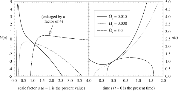
Figure 4: The cosmological potential $V(a)$ for the special case discussed in Sec. III.2 (left) along with the associated numerical solutions (right). We have taken $\Omega_{x}=0.3$. As indicated in the left panel, the $\Omega_{y}=3.0$ potential curve has been scaled by a factor of 4 to highlight the existence of the (shallow) barrier. The numeric solutions are calibrated so that the scale factor at the current time is unity.

We conclude the present analysis by presenting analytic expressions that allow one to predict the qualitative behaviour of the scale factor solutions given the values of $(\Omega_{x},\Omega_{y})$. This problem reduces to characterizing the behaviour of a cubic polynomial and is presented in detail elsewhere Seahra et al. (2003); Seahra (2003); here, we merely present the results. Consider the following three conditions:

$$h_{1}: 4\Omega_{y}-(\Omega_{x}+2\Omega_{y})^{2}>0,$$ (52a)

$$h_{2}: \left[(\Omega_{x}+2\Omega_{y})^{2}-4\Omega_{y}\right]^{3/2}-27\Omega_{x}\Omega_{y}^{2}>0,$$ (52b)

$$h_{3}: (\Omega_{x}+2\Omega_{y})^{2}-4\Omega_{y}-9\Omega_{x}^{2}>0.$$ (52c)

The origin and fate of the brane universe depends on whether these hypotheses are true or false, as communicated in Table 1. We plot these inequalities in the $\mathcal{P}^{2}$ parameter space in Figure 5.

Conditions		$h_{3}$ true	$h_{3}$ false
$h_{1}$ true		big bang & eternal expansion (I)
$h_{1}$ false	$h_{2}$ true	big bang & crunch (II)	big bounce (III)
	$h_{2}$ false	big bang & eternal expansion (IV)

Table 1: The qualitative behaviour of the special brane cosmology discussed in Section III.2. The origin and fate of the universe is determined by whether the $\{h_{1},h_{2},h_{3}\}$ hypotheses are true or false.

Figure 5: The $\mathcal{P}^{2}=(\Omega_{1},\Omega_{2})$ parameter space for the special brane cosmology discussed in Section III.2. The four regions (I)–(IV) are defined in Table 1; for example, if $(\Omega_{1},\Omega_{2})$ lies within region (III) then we know that we have a big bounce cosmology. Notice that the only region where the bulk black holes have positive mass is region (I).

To summarize, in this subsection we have examined the classical cosmology of a special case of our model. The case considered is characterized by $d=3$, a vanishing bulk cosmological constant, and spatially flat submanifolds ${\mathbb{S}}_{d}^{(k)}=S_{3}^{(0)}$. We took the matter on the brane to be given by a dust population plus a vacuum energy contribution. We found that the potential governing the brane’s motion could have classically forbidden regions if the bulk black hole has negative mass. Finally, we showed that the parameter space labelling solutions of the Friedmann equation was 2-dimensional, and we analytically determined the origin and fate of the universe on the brane based on the values of those parameters.

We finish by noting that despite the fact that the preceding scenario seems somewhat contrived, it is not wholly unphysical. We do indeed live in a 4-dimensional universe that appears to be spatially flat and contains a vacuum energy and cosmological dust. Indeed, from the point of view of observational cosmology, a simplistic model for our universe could be realized by setting the dust density parameter $\Omega_{x}=0.3$ and the amplitude of the quadratic correction to be $\Omega_{y}\ll 1$, which is necessary to avoid messing up nucleosynthesis. The dark matter in such a model comes from the Weyl contribution $\Omega_{w}$. The only thing that seems strange is our allowance for negative mass in the bulk. We will not attempt to argue that this is or is not reasonable, other than to reflect on fact that in order to realize classically forbidden regions in standard cosmology, one often needs to break the energy conditions. At least in this special case, this truism carries over to the brane world scenario.

III.3 Instanton trajectories and tachyonic branes

We conclude our analysis of the classical mechanics of our model by wandering into the semi-classical regime and considering brane instanton trajectories. We are especially interested in showing how the presence of the bulk black holes alters the archetypical example of the quantum birth of the universe: namely the deSitter FLRW model with spherical spatial sections treated in the semi-classical approximation. We also consider classical trajectories that traverse the tachyon region, and find that such paths can only be realized if the branes density is allowed to become imaginary.

For this section, let us also choose $d=3$, set the lapse equal to unity, and the matter content of the brane to be that of a single perfect fluid with equation of state $p=\gamma\rho$. Then the classical brane trajectory can be written as

$$\alpha_{m}^{2}\rho_{0}^{2}=a^{2(3\gamma+2)}\left[\left(\frac{da}{dt}\right)^{2}+F(a)\right].$$ (53)

Here, $\rho_{0}$ is a constant that controls the amplitude of the matter field. Instanton trajectories can be found from this by making the switch to the Euclidean time $t\rightarrow i\tau_{E}$. The ordinary $k=1$ deSitter model is found by setting $K=\Lambda=0$ and $\gamma=-1$. To construct the trajectory of a universe that is “created from nothing”, we replace the classical trajectory with the instanton trajectory whenever $da/dt<0$. The brane’s path through configuration space for this setup is shown in the left panel of Fig. 6 for several different values of $\alpha_{m}^{2}\rho_{0}^{2}$ ranging from $0$ to $0.4$. In this plot we see the familiar behaviour of the deSitter instanton; all of the Euclidean trajectories interpolate between the ordinary expanding universe and a universe of zero radius, which is the “nothing” state. Now what happens if we turn on the bulk black hole mass? We set $K=\tfrac{1}{2}$ and replot the trajectories for the same choices of $\alpha_{m}^{2}\rho_{0}^{2}$ in the right panel of Fig. 6. Now the instanton trajectories interpolate between an expanding state with a conventional big bang and an eternally expanding universe. Essentially, the black holes create a classically allowed region around the singularity that is not present in the archetypical case. Physically, one can understand this by realizing that the gravitational attraction of the black hole is in direct competition with the tendency of a spherical shell of vacuum energy to inflate. The important thing is that the black holes essentially expels the instanton paths from the $a=0$ area, breaking up the creation from nothing picture.

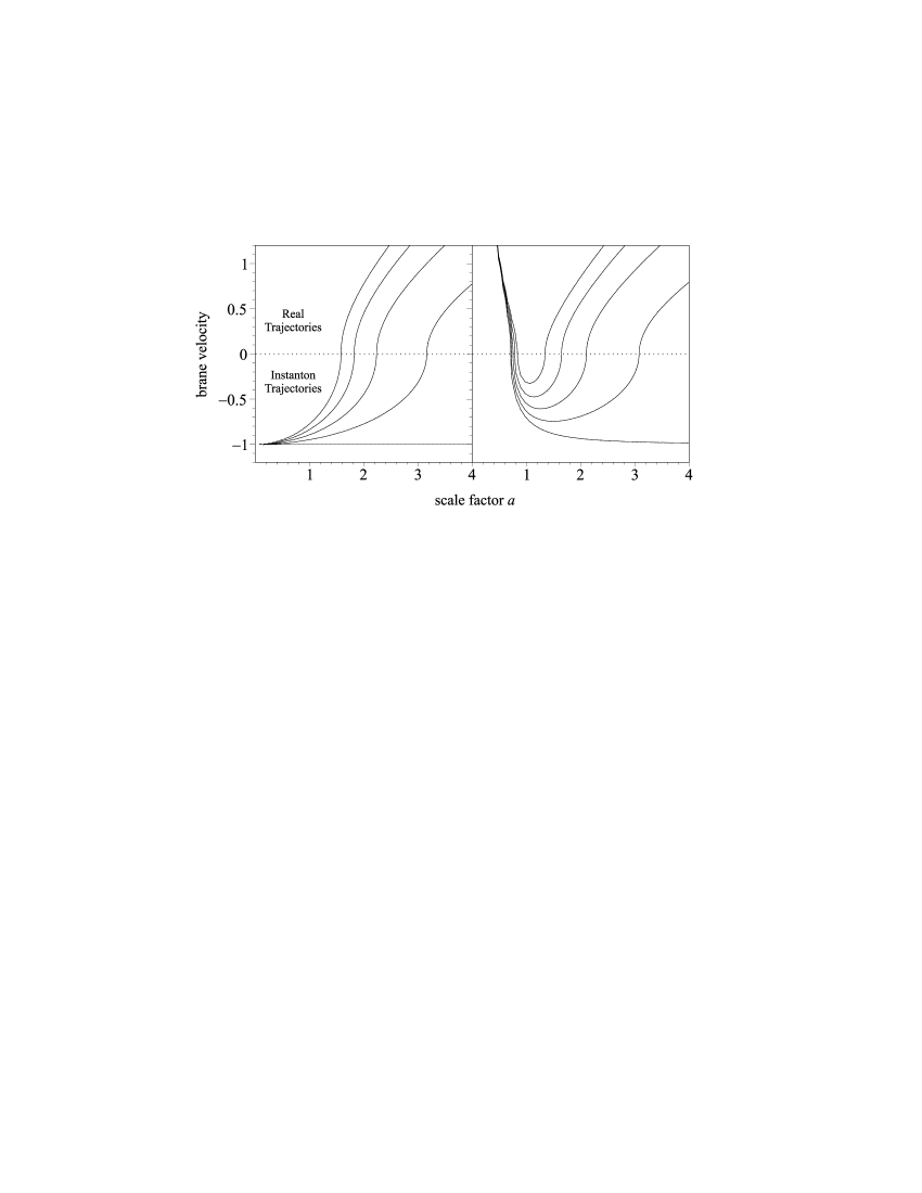
Figure 6: The trajectory of spherical 3-branes through configuration space for the case where $\Phi=1$ and the brane contains only vacuum energy. Different curves correspond to $\alpha_{m}^{2}\rho_{0}^{2}=0,0.1,0.2,0.3,0.4$ from bottom to top. The left panel shows the canonical deSitter instanton with $K=\Lambda=0$ while the right panel shows how the trajectories are deformed when $K=\tfrac{1}{2}$.

It is interesting to note that in Fig. 6 that the instanton trajectories do not seem to intersect the tachyon region. One can confirm that this is true in all situations by applying the Wick rotation of the time to inequality (35):

$$F(a)>\frac{1}{\Phi^{2}}\left(\frac{da}{d\tau_{E}}\right)^{2}.$$ (54)

So, we see that the Euclidean trajectory only exists for $F(a)>0$; i.e., in the exterior region. This is strange because we usually associate instanton trajectories with all of the classically forbidden regions of a model; clearly, the tachyon region is a special kind of forbidden region and actually represents an insurmountable boundary at the semi-classical level. Again this makes sense when we realize that the brane would have to become spacelike if it entering the tachyon region; it seems as if there is no semi-classical amplitude for such a transition. This also suggests how we might be able to find trajectories inside the region. Suppose that the brane is populated by tachyonic matter; i.e., matter with imaginary density $\alpha_{m}^{2}\rho^{2}_{0}<0$. In that case we find that

$$0>\frac{\dot{a}^{2}}{\Phi^{2}}+F(a),$$ (55)

which means that the trajectory is entirely contained within the tachyon region. We plot some of the configuration space trajectories of branes containing real and tachyonic dust and vacuum matter in Fig. 7. Again we set $d=3$ and $\Phi=1$, we also choose $K=1$ and $\Lambda=\tfrac{1}{2}$. While the branes with real dust go through a big bang and big crunch, the branes with tachyonic dust are seen to go through periodic expansion and contraction. In contrast, branes with real vacuum energy begin with a big bang and expand for ever (or vice versa) while branes with imaginary vacuum energy go through a big bang and big crunch.

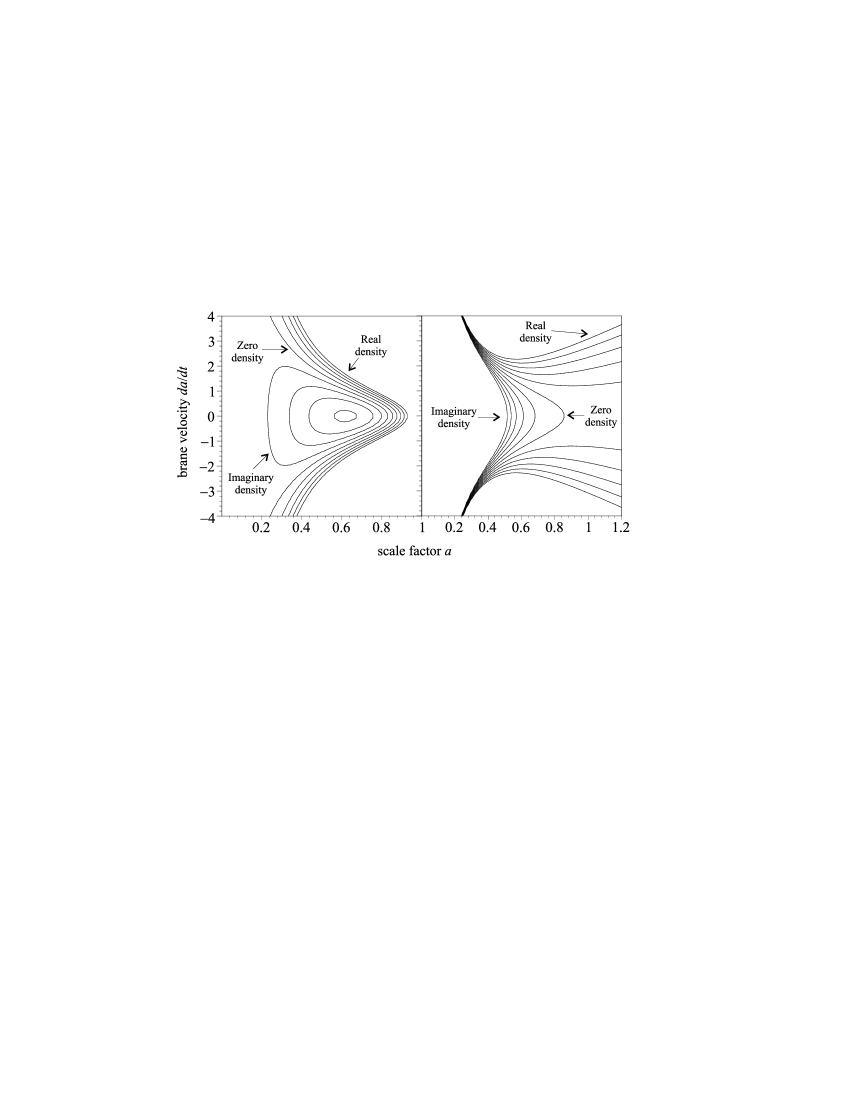
Figure 7: The trajectory of spherical 3-branes containing real and tachyonic matter through configuration space. We set $\Phi=1$, $K=1$ and $\Lambda=\tfrac{1}{2}$. The left panel shows dust filled branes with $\alpha_{m}^{2}\rho_{0}^{2}$ ranging from $-0.2$ to $+0.2$. The right panel shows vacuum dominated branes with $\alpha_{m}^{2}\rho_{0}^{2}$ ranging from $-10$ to $+10$.

In conclusion, in this section we have considered the instanton trajectories of spherical vacuum 3-branes, some of which are plotted in Fig. 6. We have seen how the presence of the bulk black holes ruins the “creation from nothing” scenario associated with the purely 4-dimensional FLRW model. We have also seen that the only way to find brane trajectories that pass through the tachyon region is to have tachyonic matter on the brane. Such paths are shown with their conventional counterparts in Fig. 7.

IV Hamiltonian formalism and the quantum cosmology

We now want to pass over from the variational formalism used up to this point to the Hamiltonian structure needed to quantize our model. But we immediately run into an ambiguity due to the fact that we have at least three different actions that we can use to Hamiltonize the model. The simplest thing to do is just choose one action — $S$ say — and ignore the others. But the fact that $S$ is complex in the interior region means that the momenta derived from $S$ are complex there too. So if we decide to use $S$ to describe the dynamics of the brane throughout configuration space we are forced to deal with a complex phase space. There is a similar problem with using either $S_{\pm}$ as the exclusive action for the model. While the issue of complex phase space in and of itself is intriguing, we are not looking for that level of complication in the current study. So we pursue an alternative line of attack: we simply take the action of the model to be defined in a piecewise fashion over configuration space; i.e., we take $S$ in the exterior region and $S_{\pm}$ in the white/black hole regions. The hope is that the Wheeler-DeWitt equation arising from each of the actions will match smoothly across the boundary between these regions. After a suitable manipulation of the constraints, we will see that this hope can be borne out. We first carry out the Hamiltonization in the exterior region, and then do the same for the interior regions — the procedures are virtually identical.

IV.1 The exterior region

In the exterior region, we can describe our system by one action $S=\int dt\,L$, given by equation (17), and we may assume $\sqrt{F}\in\mathbb{R}^{+}$. We define the model’s Lagrangian by

$$L = L_{g}+\alpha_{m}L_{m},$$ (56a)

$$L_{g} = \Phi a^{d-1}\left[-\frac{\dot{a}}{\Phi}\mathrm{arcsinh}\left(\frac{\dot{a}}{\Phi\sqrt{F}}\right)+\sqrt{\frac{\dot{a}^{2}}{\Phi^{2}}+F}\right],$$ (56b)

$$L_{m} = \Phi a^{d}{\mathcal{L}}_{m}.$$ (56c)

The canonical momenta conjugate to the scale factor and lapse function are simply found:

$$p_{a}\equiv\frac{\partial L}{\partial\dot{a}}=-a^{d-1}\mathrm{arcsinh}\left(\frac{\dot{a}}{\Phi\sqrt{F}}\right),\quad p_{\Phi}\equiv\frac{\partial L}{\partial\dot{\Phi}}=0.$$ (57)

The second of these is a primary constraint on our system:

$$\varphi_{0}=p_{\Phi}\sim 0.$$ (58)

We use Dirac’s notation that a “$\sim$” sign indicates that equality holds weakly; i.e., after all constraints have been imposed. The definition of $p_{a}$ can be rewritten as

$$\sqrt{F}\cosh\left(\frac{p_{a}}{a^{d-1}}\right)=\sqrt{\frac{\dot{a}^{2}}{\Phi^{2}}+F}.$$ (59)

The total Hamiltonian of the model is defined by

$$H = H_{g}+\alpha_{m}H_{m},$$ (60a)

$$H_{g} = p_{a}\dot{a}-L_{g}$$ (60b)

$$H_{m} = \sum_{i}\pi_{i}\dot{\psi}_{i}-L_{m}\equiv\Phi a^{d}{\mathcal{H}}_{m}.$$ (60c)

Here, we have defined $\pi_{i}$ as the momentum conjugate to the matter fields $\psi_{i}$; i.e., $\pi_{i}=\partial L_{m}/\partial\dot{\psi}_{i}$. Also note our definition of the matter Hamiltonian density ${\mathcal{H}}_{m}$. Making use of (59), we obtain

$$H=\Phi a^{d-1}\left[-\sqrt{F}\cosh\left(\frac{p_{a}}{a^{d-1}}\right)+\alpha_{m}a{\mathcal{H}}_{m}\right].$$ (61)

At this juncture, we should say a few words about the matter sector of the model. Note that relativistic invariance implies that all the matter field velocities in the matter Lagrangian must be divided by the lapse function. This is because $\Phi\,dt$ is an invariant but $dt$ by itself is not. By the same token, $\Phi$ by itself is not an invariant, so we do not expect to see any appearances of $\Phi$ uncorrelated with a velocity. Therefore, instead of regarding ${\mathcal{L}}_{m}$ as a function of $\dot{\psi}_{i}$ and $\Phi$ separately, we can instead regard it as a function of $v_{i}=\dot{\psi}_{i}/\Phi$, which may be thought of as the proper velocity of matter fields. We can then define an alternative Lagrangian density by ${\mathcal{L}}_{m}(\psi_{i},\dot{\psi}_{i};a,\Phi)=\bar{{\mathcal{L}}}_{m}(\psi_{i},v_{i};a)$. The canonical momenta definition becomes

$$\pi_{i}=a^{d}\frac{\partial\bar{\mathcal{L}}_{m}}{\partial v_{i}}.$$ (62)

We can use this with $\partial v_{i}/\partial\Phi=-\dot{\psi}_{i}/\Phi^{2}$ to deduce that

$${\mathcal{L}}_{m}+\Phi\frac{\partial{\mathcal{L}}_{m}}{\partial\Phi}=-a^{-d}\sum_{i}\pi_{i}v_{i}+{\mathcal{L}}_{m}=-{\mathcal{H}}_{m}.$$ (63)

Comparing this with (33) gives the result

$${\mathcal{H}}_{m}=\rho_{\mathrm{tot}}.$$ (64)

This is sensible; the Hamiltonian density of the matter is equal to its total matter-energy density on solutions. Since $\rho_{\mathrm{tot}}$ is a physical observable it ought to be independent of the lapse function, which is a gauge-dependent quantity. This can be rigorously shown by noting that the Hamiltonian density may be written as

$${\mathcal{H}}_{m}(\psi_{i},\pi_{i};a,\Phi)=a^{-d}\sum_{i}\pi_{i}v_{i}-\bar{\mathcal{L}}_{m}(\psi_{i},v_{i};a).$$ (65)

If the definition of the canonical momenta (62) is used to replace all instances of $v_{i}$ with expressions involving $(\psi_{i},\pi_{i};a)$ — which should always be possible — this implies that

$$\frac{\partial{\mathcal{H}}_{m}}{\partial\Phi}=0\quad\Rightarrow\quad{\mathcal{H}}_{m}={\mathcal{H}}_{m}(\psi_{i},\pi_{i};a).$$ (66)

The last point is that even though we can remove all functional dependence of ${\mathcal{H}}_{m}$ on the proper velocities, we cannot necessarily find explicit expressions for $v_{i}=v_{i}(\psi_{i},\pi_{i};a)$. This will only be possible if (62) is invertible, which requires that the Hessian determinant of the system be non-vanishing:

$$\det\left(\frac{\partial^{2}\bar{\mathcal{L}}_{m}}{\partial v_{i}\partial v_{j}}\right)\neq 0.$$ (67)

If this fails, the matter Lagrangian is said to be singular and we will have some number of primary constraints on the matter coordinates and momenta $\chi^{(1)}_{r}\sim 0$ Gitman and Tyutin (1990). One obtains explicit representations of these by manipulating the system of equations (62) to eliminate the velocities, which means that any primary constraints are independent of the lapse and $p_{a}$; i.e., $\chi^{(1)}_{r}=\chi^{(1)}_{r}(\psi_{i},\pi_{i};a)$. Can we make the simplifying assumption that all of the matter Lagrangians that we are interested in are nonsingular? The answer is no, largely because such an assumption would forbid the existence of gauge fields — which always involve constraints — living on the brane, and is therefore too restrictive.

So, to summarize, we have written down the Hamiltonian of the model (61) and found out there is at least one primary constraint $\varphi_{0}\sim 0$. Other primary constraints $\chi^{(1)}_{r}\sim 0$ may come from the matter sector. The next step is to construct the extended Hamiltonian

$$H^{\prime}=H+\mu_{0}\varphi_{0}+\sum_{r}\lambda^{(1)}_{r}\chi^{(1)}_{r},$$ (68)

where $\mu_{0}$ and $\lambda^{(1)}_{r}$ are coefficients yet to be determined. Time derivatives of any quantity are computed through the usual Poisson bracket:

$$\dot{A}\sim\{A,H^{\prime}\}.$$ (69)

We now attempt to enforce that the time derivative of $\varphi_{0}$ is zero. Making note that both ${\mathcal{H}}_{m}$ and $\chi^{(1)}_{r}$ are independent of $\Phi$, we see that $\dot{\varphi}_{0}=0$ implies the existence of an additional constraint:

$$\xi=-\sqrt{F}\cosh\left(\frac{p_{a}}{a^{d-1}}\right)+\alpha_{m}a{\mathcal{H}}_{m}\sim 0.$$ (70)

This gives that our original Hamiltonian is proportional to a constraint $H=\Phi\xi$ and therefore vanishes weakly, which is characteristic of reparametrization invariant systems. The first-stage Hamiltonian of our model is then defined as

$$H^{(1)}=\mu_{0}\varphi_{0}+\mu_{1}\xi+\sum_{r}\lambda^{(1)}_{r}\chi^{(1)}_{r},$$ (71)

where $\mu_{1}$ is yet another undetermined coefficient.

Now, let us turn our attention to the $\chi^{(1)}$ constraints. We must demand that each of these is conserved in time, which leads to the condition $\{\chi^{(1)}_{r},H^{(1)}\}\sim 0$. This in turn can generate new constraints $\chi^{(2)}\sim 0$, which then defines a new second stage Hamiltonian $H^{(2)}$. But then we need to demand that $\chi^{(2)}$ be conserved, which can generate even more constraints $\chi^{(3)}\sim 0$. Eventually the algorithm will terminate, say at the $q^{\mathrm{th}}$ stage, when demanding that $\{\chi_{r}^{(q)},H^{(q)}\}\sim 0$ does not general any new constraints. Now, by performing a linear transformation on the $q^{\mathrm{th}}$ stage matter constraints, we can divide them into two sets defined by

$$\chi^{(q)} = \varrho^{(q)}\cup\varpi^{(q)}=(\varrho^{(q)}_{1},\varrho^{(q)}_{2},\dots,\varpi^{(q)}_{1},\varpi^{(q)}_{2},\ldots),$$ (72a)

$$0 \sim \{\varrho^{(q)}_{I},\varrho^{(q)}_{J}\},$$ (72b)

$$0 \sim \{\varrho^{(q)}_{I},\varpi^{(q)}_{R}\},$$ (72c)

$$0 \nsim \det\{\varpi^{(q)}_{R},\varpi^{(q)}_{S}\}.$$ (72d)

Here, middle and late uppercase Latin indices run over the $\varrho^{(q)}$ and $\varpi^{(q)}$ constraints respectively. The $q^{\mathrm{th}}$ stage Hamiltonian is then

$$H^{(q)}=\mu_{0}\varphi_{0}+\mu_{1}\xi+\sum_{I}a^{(q)}_{I}\varrho^{(q)}_{I}+\sum_{R}b^{(q)}_{R}\varpi^{(q)}_{R},\quad\dot{A}\sim\{A,H^{(q)}\},$$ (73)

where the $a^{(q)}$ and $b^{(q)}$ coefficients are undetermined. Most importantly, it can be shown that all of the members of the $\varrho^{(q)}$ and $\varpi^{(q)}$ sets are independent of $\Phi$.

We now have the complete set of constraints for our model: $\varphi_{0}$, $\xi$, $\varrho^{(q)}$, and $\varpi^{(q)}$. According to Dirac Dirac (1964); Gitman and Tyutin (1990), the next step is to categorize them as first-class and second-class constraints. It is obvious that $\varphi_{0}$ is first-class since we have already established that it commutes with the other constraints under the Poisson bracket. It is also obvious that since $0\nsim\det\{\varpi^{(q)}_{R},\varpi^{(q)}_{S}\}$, the $\varpi^{(q)}$ constraints are second-class. Furthermore, we have by construction that the $\varrho^{(q)}$ constraints commute among themselves and the $\varpi^{(q)}$ set. Also, since the constraint-generating procedure ends at the $q^{\mathrm{th}}$ stage, all of the members of $\varrho^{(q)}$ set must commute with $\xi$, so they are all first-class constraints. Using these facts allows us to solve for the $b^{(q)}$ coefficients explicitly by setting $\dot{\varpi}_{R}^{(q)}=0$:

$$b_{R}^{(q)}=-\sum_{S}\{\varpi^{(q)}_{R},\varpi^{(q)}_{S}\}^{-1}\{\varpi^{(q)}_{S},\mu_{1}\xi\}.$$ (74)

Here, we have defined $\{\varpi^{(q)}_{R},\varpi^{(q)}_{S}\}^{-1}$ as the matrix inverse of $\{\varpi^{(q)}_{S},\varpi^{(q)}_{P}\}$ such that

$$\delta_{RP}=\sum_{S}\{\varpi^{(q)}_{R},\varpi^{(q)}_{S}\}^{-1}\{\varpi^{(q)}_{S},\varpi^{(q)}_{P}\}.$$ (75)

The only thing left is $\xi$ itself. Without knowing more about the $\varpi^{(q)}$ constraints, we cannot say with certainty that they do or do not commute with $\xi$ under the Poisson bracket. (If they did, then $b_{R}^{(q)}\sim 0$.) But this ignorance is not really important if we move over to the Dirac bracket formalism. We define the Dirac bracket between two phase space functions as

$$\{A,B\}_{*}=\{A,B\}-\sum_{RS}\{A,\varpi^{(q)}_{R}\}\{\varpi^{(q)}_{R},\varpi^{(q)}_{S}\}^{-1}\{\varpi^{(q)}_{S},B\}.$$ (76)

So defined, the Dirac bracket has the same basic properties as the Poisson bracket; i.e., it is antisymmetric in its arguments, it satisfies the Jacobi identity, etc. Under the Dirac bracket, each of the $\varpi^{(q)}$ constraints commute with every phase space function strongly:

$$\{A,\varpi^{(q)}_{R}\}=0.$$ (77)

This implies that we can impose $\varpi^{(q)}_{R}=0$ as a strong equality; i.e., we can use the second-class constraints to simplify the first-class constraints. Also, the Hamiltonian can be written in a more streamlined form:

$$H_{\mathrm{tot}}=\mu_{0}\varphi_{0}+\mu_{1}\xi+\sum_{I}a^{(q)}_{I}\varrho^{(q)}_{I},\quad\dot{A}\sim\{A,H_{\mathrm{tot}}\}_{*}.$$ (78)

It is easy to confirm that the time evolution equation under the Dirac bracket using $H_{\mathrm{tot}}$ is the same as the one under the Poisson bracket (73) if one makes use of (74). Also under the Dirac bracket, both $\xi$ and $H_{\mathrm{tot}}$ are realized as first-class quantities. Finally, the coefficients $\mu_{0}$, $\mu_{1}$, and $a^{(q)}$ are completely arbitrary and hence represent the gauge freedom of the system.

If we wanted to proceed with the Dirac quantization of the model at this point, we would promote the Dirac brackets to operator commutators, choose a representation, and then restrict the physical Hilbert space by demanding that all state vectors be annihilated by the first-class constraints. The only impediment to the immediate implementation of this procedure is the functional form of $\xi$. As written, $\xi$ contains a hyperbolic function of $p_{a}$. This will be problematic if we choose the standard operator representation $\hat{p}_{a}=i\partial/\partial a$ because the operator $\hat{\xi}$ will contain $\partial/\partial a$ to all orders, essentially resulting in an infinite-order partial differential equation. There are two ways to remedy this; we could choose a non-standard operator representation, or we can try to rewrite the constraint in a different way at the classical level. Let opt for the latter strategy. From the theory of constrained Hamiltonian systems, we know that we can transform one set of constraints into another set by applying a linear transformation matrix. The only requirement is that the matrix be non-singular on the constraint surface. In this case, we want to replace a single constraint $\xi$ with an equivalent constraint $\varphi_{1}$ such that

$$\xi=0\text{ if and only if }\varphi_{1}=0.$$ (79)

The linear transformation is trivial:

$$\varphi_{1}=\frac{\varphi_{1}}{\xi}\xi.$$ (80)

Demanding that the “transformation matrix” be non-singular is equivalent to saying that

$$\frac{\varphi_{1}}{\xi}\nsim 0;$$ (81)

i.e., the ratio of the two constraints does not vanish weakly. To ensure this, it is sufficient to demand that the gradients of $\xi$ and $\varphi_{1}$ do not vanish when the constraints are imposed. It is straightforward to verify that if we select

$$\varphi_{1}=Fa^{d}\left[p_{a}^{2}-a^{2(d-1)}\mathrm{arccosh}^{2}\left(\frac{\alpha_{m}a{\mathcal{H}}_{m}}{\sqrt{F}}\right)\right],$$ (82)

then (79) and (81) are satisfied. We will discuss the reason for including the $Fa^{d}$ prefactor in this new constraint shortly. Our final form of the Hamiltonian is then

$$H_{\mathrm{tot}}=\mu_{0}\varphi_{0}+\mu_{1}\varphi_{1}+\sum_{I}a^{(q)}_{I}\varrho^{(q)}_{I}.$$ (83)

As is appropriate for reparametrization invariant systems, the Hamiltonian is a linear combination of first-class constraints.

Having completed this short detour, we are ready to quantize the model. We make the usual correspondence

$$[\hat{A},\hat{B}]=i\{A,B\}_{*}\Big{|}_{A=\hat{A},B=\hat{B}}.$$ (84)

One assumption that will make our life easier is

$$\{a,p_{a}\}_{*}=1.$$ (85)

That is, the Dirac bracket between the conjugate pair $(a,p_{a})$ is the same as the Poisson bracket. It is possible that this might not be true, because some of the $\chi^{(2)}$ and later stage constraints could involve $p_{a}$. But for any of the concrete examples of matter models that we consider, (85) will hold. In that case, we make the usual choice of operator and state representations:

$$\langle a;\psi_{i}|\hat{a}|\tilde{\Psi}\rangle = a\tilde{\Psi}(a;\psi_{i}),$$ (86a)

$$\langle a;\psi_{i}|\hat{\psi}_{i}|\tilde{\Psi}\rangle = \psi_{i}\tilde{\Psi}(a;\psi_{i})$$ (86b)

$$\langle a;\psi_{i}|\hat{p_{a}}|\tilde{\Psi}\rangle = i\frac{\partial}{\partial a}\tilde{\Psi}(a;\psi_{i}).$$ (86c)

Here, we consider $|\tilde{\Psi}\rangle$ to be a possible physical state vector for our model that is annihilated by the constraints, while $|a,\psi_{i}\rangle$ is a state of definite $a$ and $\psi_{i}$. Note that since we don’t really know much about $\{\psi_{i},\pi_{j}\}_{*}$, we have not yet specified and operator representation of the momenta conjugate to the matter fields $\hat{\pi}_{i}$. Also, we implicitly assumed that $\tilde{\Psi}$ is independent of $\Phi$, which means the constraint $\hat{\varphi}_{0}|\tilde{\Psi}\rangle=0$ is satisfied immediately if we select $\hat{p}_{\Phi}=i\partial/\partial\Phi$. The constraint $\hat{\varphi}_{1}|\tilde{\Psi}\rangle=0$ yields the Wheeler-DeWitt equation

$$\left[-\frac{\partial}{\partial a}Fa^{d}\frac{\partial}{\partial a}-Fa^{3d-2}\mathrm{arccosh}^{2}\left(\frac{\alpha_{m}a\hat{\mathcal{H}}_{m}}{\sqrt{F}}\right)\right]\tilde{\Psi}(a;\psi_{i})=0.$$ (87)

Here, $\hat{\mathcal{H}}_{m}$ is obtained from the classical expression for ${\mathcal{H}}_{m}$ by replacing $\pi_{i}$ by its operator representation; i.e., $\hat{\mathcal{H}}_{m}={\mathcal{H}}_{m}(\psi_{i},\hat{\pi}_{i};a)$. In converting $\varphi_{1}$ into an operator, we are faced with two ordering ambiguities. One of these is relatively innocuous: Since $\partial/\partial a$ clearly does not commute with $Fa^{d}$, the relative order of the three operators in the first term on the left is non-trivial. But by demanding that the product of these operators be Hermitian, we arrive at the ordering shown above. The second ordering issue comes from the fact that we are unsure if

$$\{a,{\mathcal{H}}_{m}\}_{*}\stackrel{{\scriptstyle?}}{{=}}0.$$ (88)

If this Dirac bracket does not vanish, we have a very serious problem in the second term of the Wheeler-DeWitt equation. So we need to make another assumption, namely that the $\hat{a}$ and ${\mathcal{H}}_{m}$ operators do indeed commute. If that is true, then we can perform a separation of variables by setting

$$\tilde{\Psi}(a;\psi_{i})=\Psi(a)\Upsilon(\psi_{i}).$$ (89)

Now, consider the eigenvalue problem associated with the $\hat{\mathcal{H}}_{m}(\psi_{i},\hat{\pi}_{i};a)$ operator where we treat $a$ as a parameter. Let us select $\Upsilon$ to be an eigenfunction of $\hat{\mathcal{H}}_{m}$ so that

$$\hat{\mathcal{H}}_{m}(\psi_{i},\hat{\pi}_{i};a)\Upsilon(\psi_{i})=\mathcal{U}_{m}(a)\Upsilon(\psi_{i}).$$ (90)

Here, the “eigenvalue” is $\mathcal{U}_{m}(a)$ and should, in general, be labelled by some quantum numbers, as should $\Upsilon(\psi_{i})$. However, in the interests of brevity we will omit any such decoration. Since ${\mathcal{H}}_{m}$ is classically associated with the total matter energy density of the matter fields, what we are essentially doing is finding a basis for the physical state space in terms of state vectors of definite matter-energy density $\rho_{\mathrm{tot}}(a)=\mathcal{U}_{m}(a)$.

With the total wavefunction partitioned in the way, we can return to the Wheeler-DeWitt equation. Since by assumption $\hat{\mathcal{H}}_{m}$ and $a$ commute, we can expand the second term in (87) in a series, have $\hat{\mathcal{H}}_{m}$ act on $\Upsilon$ to produce powers of the eigenvalue, and then collapse the series into a single function. Then, we can safely divide the resulting reduced Wheeler-DeWitt equation through by $\Upsilon$. The result is similar to what we had before:

$$\left[-\frac{\partial}{\partial a}Fa^{d}\frac{\partial}{\partial a}-Fa^{3d-2}\mathrm{arccosh}^{2}\left(\frac{\alpha_{m}a\mathcal{U}_{m}}{\sqrt{F}}\right)\right]\Psi(a)=0,$$ (91)

but now we have a purely one-dimensional problem as there are no references to the matter fields or their conjugate momenta.

Let us return to the rationale for the inclusion of the $Fa^{d}$ factor. We could rewrite the Wheeler-DeWitt equation as

$$\left[-\frac{1}{a^{d}\sqrt{\sigma^{(k,d)}}}\frac{\partial}{\partial a}Fa^{d}\sqrt{\sigma^{(k,d)}}\frac{\partial}{\partial a}-Fa^{2(d-1)}\mathrm{arccosh}^{2}\left(\frac{\alpha_{m}a\mathcal{U}_{m}}{\sqrt{F}}\right)\right]\Psi(a)=0,$$ (92)

so that the volume element of the bulk manifold(s) evaluated on the brane appears in the first term. This is then equivalent to

$$[-\nabla^{A}\nabla_{A}+\mathfrak{V}]\Psi\Big{|}_{R=a}=0,$$ (93)

where $\mathfrak{V}$ and $\Psi$ are scalar functions of the bulk radial coordinate. In other words, our Wheeler-DeWitt equation is merely a scalar wave equation in the bulk manifold evaluated at the position of the brane. In keeping with the PCP, the wavefunction does not depend on the spatial coordinates $\theta$, and in keeping with the static nature of the bulk manifold, the wavefunction does not depend on the killing time coordinate $T$. Although we have only established this equality in the special $(T,\theta^{a},R)$ bulk coordinate system, we expect it to hold in all coordinate systems because (93) is a tensorial statement. The inclusion of the $Fa^{d}$ factor in $\varphi_{1}$ is crucial to this conclusion, which is why we have put it there in the first place.

Let us summarize what has been accomplished in this section. We have examined the Hamiltonian dynamics of our model exterior to the horizon. There are two constraints that come from the gravitational side of the theory, as is expected by the gauge invariance of the system. We have also allowed for any number of constraints that exist among the matter degrees of freedom on the brane, which means that our model can be used in conjunction with matter gauge theories. By introducing the Dirac bracket and transforming one of the constraints from the gravity sector, we have written the system Hamiltonian as a linear combination of first class constraints. Employing standard canonical quantization, we have at the one-dimensional Wheeler-DeWitt equation:

$$\left[-\frac{\partial}{\partial a}Fa^{d}\frac{\partial}{\partial a}-Fa^{3d-2}\mathrm{arccosh}^{2}\left(\frac{\alpha_{m}a\mathcal{U}_{m}}{\sqrt{F}}\right)\right]\Psi(a)=0.$$ (94)

The form of the differential operator on the left implies that this equation is invariant under transformations of the bulk coordinates. Here, $\mathcal{U}_{m}=\mathcal{U}_{m}(a)$ is an eigenvalue of $\hat{\mathcal{H}}_{m}(\psi_{i},\hat{\pi}_{i};a)$ with respect to the matter degrees of freedom. In the process of arriving at (94), we have made the following assumptions:

1. ${\mathcal{L}}_{m}(\psi_{i},\dot{\psi}_{i};a,\Phi)=\bar{\mathcal{L}}_{m}(\psi_{i},v_{i};a)$.

2. $\{a,p_{a}\}_{*}=1$.

3. $\{a,{\mathcal{H}}_{m}\}_{*}=0$.

The first assumption has to do with the relativistic invariance of of the matter Lagrangian. The last two have to do with the structure of the second class constraints associated with the matter fields; note that these will both be satisfied if the second class constraints $\varpi^{(k)}$ are independent of $p_{a}$.

We conclude by commenting on our choice of quantizing our system with the equivalent constraint $\varphi_{1}$ instead of the original constraint $\xi$. Clearly, it does not matter at the classical level which of the constraints we use; they both describe the same dynamics. However, this is no guarantee that the quantized model is insensitive to the choice of imposing $\xi\sim 0$ or $\varphi_{1}\sim 0$. In particular, will the physical Hilbert space defined by $\hat{\varphi}_{1}|\Psi\rangle=0$ be the same as the one defined by $\hat{\xi}|\Psi\rangle=0$? Classically, we had $\xi=\Gamma\varphi_{1}$ where $\Gamma$ is a phase space function that does not vanish weakly. Clearly, if we have the operator identity $\hat{\xi}=\hat{\Gamma}\hat{\varphi}_{1}$ the two Hilbert spaces would be identical. But there is an ordering ambiguity here, because we could also have $\hat{\xi}=\hat{\varphi}_{1}\hat{\Gamma}$, which would not result in the same Hilbert space unless $\hat{\varphi}_{1}$ and $\hat{\Gamma}$ commute. This potential inconsistency — sometimes called “quantum symmetry breaking” — is endemic in the Dirac quantization programme. There is reason to believe that it can be avoided by employing alternative quantization procedures; for example, if one converts the first-class constraints in a given system to second-class ones by adding gauge-fixing conditions, it can be shown that the associated generating functional for the quantum theory is invariant under transformations of the constraints (Gitman and Tyutin, 1990, Sec. 3.4). However, we should point out that the difference between $\hat{\Gamma}\hat{\varphi}_{1}$ and $\hat{\varphi}_{1}\hat{\Gamma}$ is necessarily of order $\hbar$, so we expect the discrepancy between the physical Hilbert spaces defined by $\xi\sim 0$ and $\varphi_{1}\sim 0$ to be unimportant at the semi-classical level.

IV.2 The interior region

When $F(a)<0$, we have two different actions to choose from for the Hamiltonization procedure: $S_{\pm}$. It turns out that it does not matter which is employed, they both result in the same Wheeler-DeWitt equation. To justify this statement, we will convert the models described by $S_{\pm}$ to their Hamiltonian forms simultaneously. The momentum conjugate to $a$ for the two actions is

$$p_{a}^{\pm}=\mp a^{d-1}\mathrm{arccosh}\left(\frac{\pm\dot{a}}{\Phi\sqrt{-F}}\right).$$ (95)

Notice that inside the tachyonic region — where $|\dot{a}|<\Phi\sqrt{-F}$ — this momentum becomes imaginary. This is what one might expect inside a traditional classically forbidden region. These expressions for $p_{a}^{\pm}$ result in the Hamiltonian functions:

$$H_{\pm}=\Phi a^{d-1}\left[\pm\sqrt{-F}\sinh\left(\frac{p_{a}}{a^{d-1}}\right)+\alpha_{m}a{\mathcal{H}}_{m}\right].$$ (96)

Here, ${\mathcal{H}}_{m}$ is defined in exactly the same way as before. For both Hamiltonians, we still have the primary constraint $\varphi_{0}=p_{\Phi}\sim 0$ representing the time reparametrization invariance of the model. Demanding that this constraint is conserved in time yields the secondary constraint(s)

$$\xi_{\pm}=\pm\sqrt{-F}\sinh\left(\frac{p_{a}}{a^{d-1}}\right)+\alpha_{m}a{\mathcal{H}}_{m}.$$ (97)

At this point we need to repeat the constraint generating and classification procedure described in the previous subsection. Now, since the first stage matter constraints $\chi^{(1)}$ are determined entirely by the matter Lagrangian, we expect that they will be the same inside and outside the horizon. However, the higher stage constraints $\chi^{(2,3,\ldots)}$ are obtained by commuting various expressions with $\xi_{\pm}$, which means that there is no reason to believe that those constraints match their counterparts outside the horizon. Hence, it is conceivable that the Dirac brackets derived from the $S$ and $S_{\pm}$ actions might be distinct from one another, which may complicate the quantization procedure. Such difficulties will be minimized if we make the assumptions:

1. $\{a,p_{a}\}^{\pm}_{*}=1$.

2. $\{a,{\mathcal{H}}_{m}\}^{\pm}_{*}=0$.

3. $\{\psi_{i},\pi_{j}\}_{*}=\{\psi_{i},\pi_{j}\}_{*}^{\pm}$.

Here, $\{,\}_{*}^{\pm}$ are the Dirac brackets defined with respect to $S_{\pm}$. This first two assumptions are the same as the ones made in the previous subsection carried over to the other side of the horizon. The third will ensure that we can choose the same operator representations for $\hat{\psi}_{i}$ and $\hat{\pi}_{i}$ inside and outside the horizon. At the end of the day, we arrive at the final Hamiltonian(s)

$$H^{\pm}_{\mathrm{tot}}=\mu_{0}\varphi_{0}+\mu_{1}\xi_{\pm}+\sum_{I}a^{(q)}_{I}\varrho^{(q)\pm}_{I},\quad\dot{A}\sim\{A,H_{\mathrm{tot}}\}^{\pm}_{*}.$$ (98)

Here, $\varrho^{(q)\pm}$ is the complete set of matter-related first class constraints derived from $S_{\pm}$. As before, the Hamiltonian is a linear combination of first class constraints that we will impose as restrictions on physical state vectors.

The last step before quantizing is to rewrite the $\xi_{\pm}$ constraints in a more useful form. It is not hard to see that an equivalent constraint is

$$\varphi_{1}^{\pm}=Fa^{d}\left[p_{a}^{2}-a^{2(d-1)}\mathrm{arcsinh}^{2}\left(\frac{\alpha_{m}a{\mathcal{H}}_{m}}{\sqrt{-F}}\right)\right]\sim 0.$$ (99)

The operator version on this constraints yields the Wheeler-DeWitt equation inside the horizon. Notice that there is no sign ambiguity on the righthand side, which means that both of $S_{\pm}$ lead to the same wave equation. To obtain this explicitly, we make the same choice of representation as we made on the other side of the horizon. After separation of variables, we obtain

$$\left[-\frac{\partial}{\partial a}Fa^{d}\frac{\partial}{\partial a}-Fa^{3d-2}\mathrm{arcsinh}^{2}\left(\frac{\alpha_{m}a\mathcal{U}_{m}}{\sqrt{-F}}\right)\right]\Psi(a)=0.$$ (100)

Here as before, $\mathcal{U}_{m}(a)$ represents an eigenvalue of the operator $\hat{\mathcal{H}}_{m}(\psi_{i},\hat{\pi}_{i};a)$. Notice that since we chose the same operator representations as before, $\mathcal{U}_{m}(a)$ can be taken to be continuous across the horizon.

IV.3 The reduced Wheeler-DeWitt equation and the quantum potential

Now that we have obtained Wheeler-DeWitt equations (94 and 100) valid inside and outside the horizon, we can examine how they are stitched together. The following definitions are quite useful:

$$\Psi(a)\equiv\frac{\Theta(a)}{a^{d/2}},\quad a_{*}\equiv a_{*}(a),\quad\frac{da_{*}}{da}\equiv\frac{1}{|F(a)|}.$$ (101)

The $a_{*}$ coordinate is the higher-dimensional generalization of the Regge-Wheeler tortoise coordinate. Written in terms of these quantities, the entire Wheeler-DeWitt equation takes the form

$$0 = -\frac{1}{2}\frac{d^{2}\Theta}{da_{*}^{2}}+U(a)\Theta$$ (102a)

$$U(a) = \frac{1}{2}F\left[\frac{d}{2a}\frac{dF}{da}+\frac{d(d-2)}{4}\frac{F}{a^{2}}-Fa^{3d-2}W(a)\right],$$ (102b)

$$W(a) = \begin{cases}\mathrm{arccosh}^{2}\left(\frac{\alpha_{m}a\mathcal{U}_{m}}{\sqrt{F}}\right),&F(a)>0,\\ \mathrm{arcsinh}^{2}\left(\frac{\alpha_{m}a\mathcal{U}_{m}}{\sqrt{-F}}\right),&F(a)<0.\end{cases}$$ (102c)

On an operational level, this is just a one-dimensional Schrödinger equation with a piecewise continuous potential $U(a)$ and zero energy. Note that as usual for covariant wave equations, the potential is an explicit function of $a$ and therefore an implicit function of $a_{*}$. Also note that if the bulk is 4-dimensional, the Wheeler-DeWitt equation reduces to the usual expression for a scalar field around a black hole subjected to a peculiar potential.

We now discuss some of the properties of the quantum potential $U(a)$. In this, we restrict our attention to matter fields with $\mathcal{U}_{m}>0$; that is, matter with positive density. We also assume that $\mathcal{U}_{m}$ is finite and well behaved for all $a\in(0,\infty)$. First and foremost, we are interested in the behaviour of the potential near a bulk horizon. To gain some insight, let us assume that all of the zeros of $F$ are simple; that is, the first derivative of $F$ does not vanish at positions where $F(a)=0$, which we denote by $a=a_{H}$. Let us focus our attention on one of these zeros where $F$ is positive to the right of $a_{H}$ and negative to the left. Near $a_{H}$, we can then approximate

$$F(a)\approx\mathcal{C}(a-a_{H}),$$ (103)

where $\mathcal{C}$ is a positive constant. Now if we take a closer look at our definition of $a_{*}$, we see that it actually defines two separate coordinate patches: one for inside the horizon $a_{*}^{\mathrm{in}}$ and one for outside the horizon $a_{*}^{\mathrm{out}}$. Then for $a\approx a_{H}$, we have

$$F(a)\approx\begin{cases}+\mathcal{C}\exp(+\mathcal{C}a_{*}^{\mathrm{out}}),&a>a_{H},\\ -\mathcal{C}\exp(-\mathcal{C}a_{*}^{\mathrm{in}}),&a<a_{H}.\end{cases}$$ (104)

From this, it is easy to see that the horizon is located at $a_{*}^{\mathrm{in}}=+\infty$ and $a_{*}^{\mathrm{out}}=-\infty$. This then yields

$$U(a)\approx\begin{cases}+\frac{\mathcal{C}^{2}d}{4a_{H}}\exp(+\mathcal{C}a_{*}^{\mathrm{out}}),&a_{*}^{\mathrm{out}}\rightarrow-\infty,\\ -\frac{\mathcal{C}^{2}d}{4a_{H}}\exp(-\mathcal{C}a_{*}^{\mathrm{in}}),&a_{*}^{\mathrm{in}}\rightarrow+\infty.\end{cases}$$ (105)

Clearly, $U(a)$ vanishes at the position of the horizon. Furthermore, all of the derivatives of $U$ with respect to $a_{*}$ (“in” or “out”) vanish there too. In other words, the quantum potential is exponentially flat and completely smooth near any bulk horizons when expressed as a function of $a_{*}$. So as far as the Wheeler-DeWitt equation is concerned, there are no artifacts left over from our adoption of a piecewise action; we just have a one-dimensional Schrödinger equation with an analytic potential.

What about the limiting behaviour of $U(a)$ for large and small $a$? The character of $U(a)$ near the singularity at $a=0$ is relatively easy to obtain if we keep in mind that if $W(a)$ diverges as $a\rightarrow 0$, that divergence goes like the square of a logarithm. We then obtain:

$$\lim_{a\rightarrow 0}U(a)=-\frac{1}{2}\left(\frac{Kd}{2a^{d}}\right)^{2}\rightarrow-\infty.$$ (106)

Therefore, the potential is infinitely attractive near the singularity, even for $K<0$. The behaviour for large $a$ is more complicated, and has to be dealt with on a case-by-case basis. The calculation is sensitive to both the values of the bulk parameters and the asymptotic behaviour of the matter density $\mathcal{U}_{m}$. We do not give details here; rather the results are listed in Table 2. We see that in general, $U(a)$ diverges to $\pm\infty$ as $a\rightarrow\infty$. The fact that $U(a)$ is unbounded from below is not unusual for quantum cosmological scenarios. As argued in ref. Feinberg and Peleg (1995), it should be addressed by the specification of boundary conditions on $\Theta$, which is an issue that we will not consider here.

			$\lim\limits_{a\rightarrow\infty}U(a)=+\infty$	$\lim\limits_{a\rightarrow\infty}U(a)=-\infty$
$\Lambda>0$			$\lim\limits_{a\rightarrow\infty}\alpha_{m}\mathcal{U}_{m}<\sqrt{\frac{2\Lambda}{d(d+1)}}$	$\lim\limits_{a\rightarrow\infty}\alpha_{m}\mathcal{U}_{m}>\sqrt{\frac{2\Lambda}{d(d+1)}}$
$\Lambda=0$	$k=+1$		$\lim\limits_{a\rightarrow\infty}\alpha_{m}a\mathcal{U}_{m}<1$	$\lim\limits_{a\rightarrow\infty}\alpha_{m}a\mathcal{U}_{m}>1$
	$k=-1$		n/a	for all $\mathcal{U}_{m}$
	$k=0$	$K>0$	n/a	for all $\mathcal{U}_{m}$
		$K<0$	$\lim\limits_{a\rightarrow\infty}\alpha_{m}a^{\frac{d+1}{2}}\mathcal{U}_{m}<\sqrt{-K}$	$\lim\limits_{a\rightarrow\infty}\alpha_{m}a^{\frac{d+1}{2}}\mathcal{U}_{m}>\sqrt{-K}$

Table 2: The large $a$ limits of $U(a)$ for various model parameters

Finally, one can verify using identity (26a) that

$$W(a)\begin{cases}>0,&F(a)<\alpha_{m}^{2}a^{2}\mathcal{U}_{m}^{2},\\ <0,&F(a)>\alpha_{m}^{2}a^{2}\mathcal{U}_{m}^{2}.\end{cases}$$ (107)

Notice how the conditions on the right mirror our previous definitions of classically allowed and classically forbidden regions (39) when $\mathcal{U}_{m}$ is identified with $\rho_{\mathrm{tot}}$. This means that the contribution to the quantum potential from $W(a)$ is positive in classically forbidden regions and negative in classically allowed regions, tending to promote non-oscillatory and oscillatory behaviour in the brane universe’s wavefunction respectively. However, the terms that do not involve $W(a)$ in $U(a)$ prevent this from being a hard and fast rule.

To summarize, in this section we have written down the Wheeler-DeWitt equation for the brane in a form identical to a Schrödinger equation with zero total energy. We have discussed the general properties of the potential $U(a)$ appearing in this equation and shown that Wheeler-DeWitt equation is analytic at the position of any bulk horizons. Finally, we saw that the quantum potential tends to be positive in the non-tachyon classically forbidden regions identified in Sec. III, but the presence of curvature-induced terms muddles this conclusion somewhat.

IV.4 Perfect fluid matter on the brane

We now specialize to the case where there is only perfect fluid matter living on the brane. For simplicity, we will first assume that there is only one fluid living on the brane and then make the trivial generalization to multi-fluid models.

The Lagrangian density for a single irrotational fluid with equation of state $p=\gamma\rho$ is given in Appendix A. When this is specialized to our metric ansatz on the brane, we have

$${\mathcal{L}}_{m}=\frac{1}{2}\left[e^{(1-\gamma)\vartheta}\frac{\dot{\psi}^{2}}{\Phi^{2}}-e^{(1+\gamma)\vartheta}\right].$$ (108)

A priori, we see two matter degrees of freedom: $\psi$ and $\vartheta$. Note that this Lagrangian meets our relativistic invariance requirement; i.e., all time derivatives are divided by $\Phi$. The conjugate momenta are

$$\pi_{\psi}=\frac{\partial}{\partial\dot{\psi}}\Phi a^{d}{\mathcal{L}}_{m}=\Phi^{-1}a^{d}e^{(1-\gamma)\vartheta}\dot{\psi},\quad\pi_{\vartheta}=\frac{\partial}{\partial\dot{\vartheta}}\Phi a^{d}{\mathcal{L}}_{m}=0.$$ (109)

The second of these is the sole primary constraint coming from the matter sector. Since it obviously commutes with itself, the constraint can immediately be classified as one of the $\varrho$ type. Hence the complete set of first stage constraints from the matter sector is

$$\varrho^{(1)}=\pi_{\vartheta}\sim 0.$$ (110)

From the expressions for the canonical momenta, ${\mathcal{H}}_{m}$ is easily obtained:

$${\mathcal{H}}_{m}=\tfrac{1}{2}[e^{-(1-\gamma)\vartheta}a^{-2d}\pi_{\psi}^{2}+e^{(1+\gamma)\vartheta}].$$ (111)

Now, the next step is to demand that $\varrho^{(1)}$ is conserved in time. According to the prescription given in the previous two sections, this involves taking the Poisson bracket of $\varrho^{(1)}$ with one of $\xi$ or $\xi_{\pm}$, depending on which portion of phase space one is working with. Fortunately, we have that

$$\{\varrho^{(1)},\xi\}=\{\varrho^{(1)},\xi_{\pm}\},$$ (112)

which means that, for the perfect fluid case, the second stage constraints associated with each of the brane actions are the same. The complete set of matter-related second stage constraints is

$$\varpi_{1}^{(2)}=\pi_{\vartheta}\sim 0,\quad\varpi_{2}^{(2)}=\pi_{\psi}-\sqrt{\frac{1+\gamma}{1-\gamma}}a^{d}e^{\vartheta}\sim 0.$$ (113)

It is easy to verify that these constraints are second class:

$$\{\varpi_{1}^{(2)},\varpi_{2}^{(2)}\}=\sqrt{\frac{1+\gamma}{1-\gamma}}a^{d}e^{\vartheta}\sim\pi_{\psi}\nsim 0.$$ (114)

Since there are no second stage first class constraints there can be no additional constraints in the system; that is, the constraint generating procedure terminates after the second stage. The Dirac bracket structure is easy to write down when there are only two second class constraints:

$$\{A,B\}_{*}\equiv\{A,B\}+\frac{\{A,\varpi_{1}^{(2)}\}\{\varpi_{2}^{(2)},B\}-\{A,\varpi_{2}^{(2)}\}\{\varpi_{1}^{(2)},B\}}{\{\varpi_{1}^{(2)},\varpi_{2}^{(2)}\}}.$$ (115)

As mentioned above, within this structure the constraints have vanishing brackets with everything else in the theory, so we can realize them as strong equalities $\varpi_{1}^{(2)}=\varpi_{2}^{(2)}=0$ and thereby simplify ${\mathcal{H}}_{m}$ by removing all references to $\vartheta$:

$${\mathcal{H}}_{m}=A_{\gamma}\pi_{\psi}^{1+\gamma}a^{-d(\gamma+1)},\quad A_{\gamma}\equiv\frac{(1-\gamma)^{(\gamma-1)/2}}{(1+\gamma)^{(\gamma+1)/2}}.$$ (116)

We can tidy this up by considering the canonical transformation

$$Q=\frac{\psi\pi_{\psi}^{-\gamma}}{A_{\gamma}(1+\gamma)},\quad P=A_{\gamma}\pi_{\psi}^{1+\gamma},$$ (117)

which yields

$${\mathcal{H}}_{m}=Pa^{-d(\gamma+1)}.$$ (118)

This is the matter Hamiltonian to be used for perfect fluids. It should be stressed that this form of the fluid Hamiltonian and the associated Dirac bracket structure is valid throughout the phase space, both inside and outside the horizon.

A few comments about the perfect fluid Hamiltonian formalism are in order: First, the perfect fluid Hamiltonian ${\mathcal{H}}_{m}=Pa^{-d(\gamma+1)}$ has been derived directly from Schutz’s variational formalism Schutz (1970a, 1971) and applied to quantum cosmology a number of times in the literature Lapchinskii and Rubakov (1977); Gotay and Demaret (1983); Lemos (1996); Acacio de Barros et al. (1998); Alvarenga and Lemos (1998); Batista et al. (2001); Alvarenga et al. (2002). Our second comment is that the total Hamiltonian of our model will be independent of $Q$, which means that $P$ is a classical constant of the motion. Therefore, on solutions ${\mathcal{H}}_{m}$ evaluates to the matter energy density of the fluid as a function of $a$ as given be equation (135); i.e., ${\mathcal{H}}_{m}=\rho(a)$. The physical interpretation of $P$ is the current time fluid density. Our final comment concerns the following Dirac brackets:

$$\{a,p_{a}\}_{*}=1,\quad\{a,{\mathcal{H}}_{m}\}_{*}=0,\quad\{Q,P\}_{*}=1.$$ (119)

The first two equalities mean our perfect fluid matter model satisfies the assumptions we made in Sec. IV.1, so we can safely use the results derived therein. The last one means that we can choose standard operator representations for $Q$ and $P$ when quantizing:

$$\langle a;Q|\hat{Q}|\tilde{\Psi}\rangle=Q\tilde{\Psi}(a;Q),\quad\langle a;Q|\hat{P}|\tilde{\Psi}\rangle=i\frac{\partial}{\partial Q}\tilde{\Psi}(a;Q).$$ (120)

Recall that in order to write down the reduced Wheeler-DeWitt equation, we need to solve the eigenvalue problem associated with $\hat{\mathcal{H}}_{m}$. With the operator representation above, that problem is trivial:

$$\hat{\mathcal{H}}_{m}\left(Q,i\frac{\partial}{\partial Q};a\right)\Upsilon(Q)=\mathcal{U}_{m}(a)\Upsilon(Q)\quad\Rightarrow\quad\Upsilon(Q)=e^{-iP_{0}Q},\,\,\,\mathcal{U}_{m}(a)=P_{0}a^{-d(\gamma+1)},$$ (121)

where $P_{0}$ is a constant. The rightmost expression can be directly substituted into equations (94) and (100) to obtain the wavefunction of the universe outside and inside the horizon respectively.

These results are easily generalized to multi-fluid models. Without going into too many details, it should be clear the Lagrangian density for a multi-fluid model is just the sum of the Lagrangian densities for each individual fluid. The Hamiltonization procedure proceeds in a fashion similar to the single fluid case, largely because the degrees of freedom for different fluids do not interact with one another. Our final result for the eigenvalue of $\hat{\mathcal{H}}_{m}$ is simply

$$\mathcal{U}_{m}(a)=\sum_{k}P_{k}a^{-d(\gamma_{k}+1)}.$$ (122)

Here, $k$ is an index that runs over all of the fluids. The $k^{\mathrm{th}}$ fluid has the equation of state $p_{k}=\gamma_{k}\rho_{k}$ and the constant $P_{k}$ represents its current epoch density. Therefore, for the multi-fluid model the eigenvalue of $\hat{\mathcal{H}}_{m}$ is the sum of the density associated with each of the fluids as a function of $a$ and the $P_{k}$ constants are the quantum numbers that label the $\Upsilon$ eigenfunction. Hence, when we put $\mathcal{U}_{m}$ into the Wheeler-DeWitt equation and solve for $\Psi(a)$, we are really solving for state of definite matter momenta. In principle, this makes $\Psi(a)$ a member of basis of matter-momentum eigenstates.

Let us move on to the quantum potential associated with fluid-filled branes. Other than the basic limiting behaviour of $U(a)$ described in the last section, the shape of $U(a)$ is hard to quantify for completely arbitrary parameter choices. So, in order to get a feel what the potential really looks like, we plot it for a wide variety of situations in Fig. 8. For these plots, we take the case of a 5-dimensional bulk $d=3$. The matter content of the brane is taken to be vacuum energy plus dust:

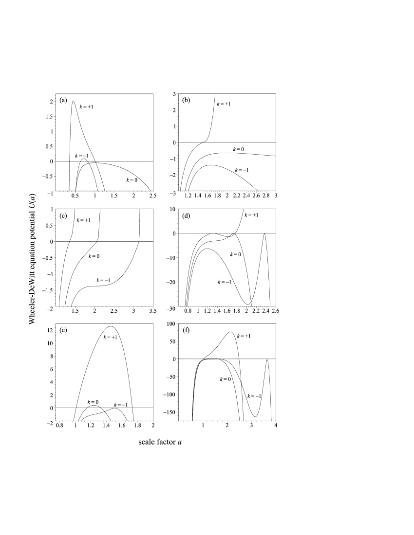
Figure 8: The potential in the Wheeler-DeWitt equation for various model parameters, which are given in Table 3.

Panel	$K$	$\Lambda$	$\rho_{\mathrm{v}}$	$\rho_{\mathrm{d}}$
(a)	$1/8$	$0$	$1/2$	$1$
(b)	$9/4$	$0$	$0$	$1/2$
(c)	$9/4$	$3/4$	$0$	$1/2$
(d)	$9/4$	$3/2$	$1/2$	$1/2$
(e)	$-9/4$	$0$	$3/4$	$1/16$
(f)	$-9/4$	$3/8$	$1/2$	$1$

Table 3: The parameter choices made in each panel of Fig. 8

$$\alpha_{m}\mathcal{U}_{m}=\rho_{\mathrm{v}}+\rho_{\mathrm{d}}a^{-3}.$$ (123)

Table 3 shows the choice of $K$, $\Lambda$, $\rho_{\mathrm{v}}$, and $\rho_{\mathrm{d}}$ made in each panel of Fig. 8. We now comment on each panel in turn:

1. The $k=+1$ curve in this panel exhibits what seems to be a finite potential barrier whose left endpoint is the horizon at $a=\tfrac{1}{\sqrt{8}}$. Notice also that the $k=-1$ potential also shows a small barrier, which is a purely quantum effect introduced by the curvature terms in the scalar wave equation; it has no classical analogue since the classical potential (equation 36) is strictly negative for this combination of parameters: $V(a)<0$.

2. The $k=+1$ curve in this plot crosses the axis at the position of the horizon at $a=\tfrac{1}{2}$. For that case, the wavefunction can be localized in the interior horizon region. For $k=0$ and $-1$, the wavefunction is delocalized over the $a$ axis.

3. All potential curves diverge to $+\infty$ in this plot because the matter density has an asymptotic value less than $\sqrt{\frac{2\Lambda}{d(d+1)}}=\tfrac{1}{8}$ (see Table 2). Any apparent “kinks” in the potential are numerical plotting artifacts; the curves are in reality completely smooth.

4. These curves correspond to a marginal case where $\lim_{a\rightarrow 0}\alpha_{m}\mathcal{U}_{m}=\sqrt{\frac{2\Lambda}{d(d+1)}}=\tfrac{1}{2}$, which is not included in Table 2. The $k=+1$ curve actually crosses the zero line three times in this case — this is somewhat hard to see without enlarging the plot — creating a legitimate potential well.

5. The bulk black holes have negative mass in this case. We see a potential barrier for the $k=0$ and $k=+1$ case. There is a horizon at $a=\tfrac{3}{2}$ for $k=-1$, which is reflected by the vanishing of the hyperbolic potential at that point.

6. All curves in this panel diverge to $-\infty$. The $k=-1$ potential goes to zero for two values of $a$, corresponding to the double horizon structure in this case. The $k=+1$ and $k=0$ potentials show barriers.

To sum up this section: we have specialized the general formalism presented in previous sections to the case where only perfect fluids are living on the brane. The $\hat{\mathcal{H}}_{m}$ operator was seen to have a very simple form, and its $\mathcal{U}_{m}(a)$ eigenvalue merely corresponds to the classical density of the fluids as a function of $a$. Also, we have provided plots for a number of different scenarios corresponding to a 3-brane containing vacuum energy and dust. Although we have tried to include as wide a sample of the different types of potentials in Fig. 8, we note that there is actually a bewildering variety of potential parameter combinations. So we must be content with the brief survey above, and we leave a more systematic study to future work.

IV.5 Tunnelling amplitudes in the WKB approximation

A number of the panels in Fig. 8 show that the curvature singularity at $a=0$ is hidden behind a potential barrier. This suggests the possibility of quantum singularity avoidance; i.e., the wavefunction of the brane can be engineered to be concentrated away from the $a=0$ region. Or conversely, we can consider the case where the brane “nucleates” by tunnelling from small to large $a$ in a sort of birth event. At a semi-classical level, the relevant quantity to both of these scenarios is the WKB tunnelling amplitude, which gives the ratio of the height of the wavefunction on either side of the barrier. If this amplitude is zero (or infinite) we see that the wavefunction can be entirely contained on one side of the barrier, while if the amplitude is close to unity it is easy to travel from one side to the other.

In our situation, the tunnelling amplitude is given by

$$T = \frac{\Psi(a_{1})}{\Psi(a_{2})}=\left(\frac{a_{2}}{a_{1}}\right)^{d/2}\frac{\Theta(a_{1})}{\Theta(a_{2})}$$ (124)

$$\propto \left(\frac{a_{2}}{a_{1}}\right)^{d/2}\exp\left(\mp\int_{a_{1}}^{a_{2}}da_{*}\,\sqrt{2U(a)}\right)$$

$$= \left(\frac{a_{2}}{a_{1}}\right)^{d/2}\exp\left(\mp\int_{a_{1}}^{a_{2}}da\,\frac{\sqrt{2U(a)}}{|F(a)|}\right).$$

Here, the potential barrier in question is assumed to occupy the interval $(a_{1},a_{2})$. The sign ambiguity in the exponential allows us to set $\Theta(a_{1})\lessgtr\Theta(a_{2})$ depending on what type of scenario we are considering. Note that we had to transform the integral of $\sqrt{2U(a)}$ from an integration over $a_{*}$ to $a$ at the price of dividing the integrand by $|F(a)|$. Now, we already know that the potential changes sign whenever $F$ changes signs, so if the bulk contains horizon(s) there will always be a potential barrier (or barriers) with a horizon as one of its endpoints. But using the asymptotic forms of $U$ and $F$ near the horizon developed in Sec. IV.3, we have that

$$\frac{\sqrt{2U(a)}}{F(a)}\propto\frac{1}{\sqrt{F}},\quad\text{for }F\gtrsim 0.$$ (125)

Hence, the integrand in $T$ has a pole at one of the integration endpoints if that endpoint represents a bulk horizon, but the pole is of order $\frac{1}{2}$. This leads us to believe that the integral is actually convergent in such cases, but this is hard to confirm numerically — partly because $W(a)$ becomes rather large near $F(a)\gtrsim 0$. We would like to report on this phenomena in the future, but for now let us restrict our discussion to calculating $T$ for cases without bulk horizons.

Since the only potential curves in Fig. 8 that exhibit barriers not bounded by horizons are associated with negative mass bulk black holes, we concentrate on the $K<0$ case. In keeping with the calculation of the last section, we again assume that the brane contains vacuum energy and dust, and $d=3$. In Fig. 9, we plot $T$ versus dust or vacuum density amplitude for a number of different situations. Note that the ratio $(a_{2}/a_{1})^{d/2}$ in the definition of $T$ means that we can have $T>1$. Two trends are apparent from this plot: $T$ increases with increasing dust or vacuum density and $T$ is usually smaller for $k=+1$ than for $k=0$. Recalling that a small value of $T$ is associated with a high potential barrier, this means that the brane’s wavefunction can be more effectively localized away from the singularity when its density is low or when its spatial sections are spherical. The former is easy to understand: when the matter on the brane is more dense, it has more gravitational self energy that promotes collapse. To understand why the barriers are higher for $k=+1$, we merely need to look at the classical potential from equation (36); the classical potential $V(a)$ increases with increasing $k$.

Figure 9: The tunnelling amplitude across the potential barrier when the black hole mass is negative: $K=-\tfrac{9}{4}$. The diamonds $(\Diamond)$ indicate the amplitude when $k=+1$, $\Lambda=0$, $\rho_{\mathrm{v}}=\tfrac{1}{2}$ and $\rho_{\mathrm{d}}$ is varied; the triangles $(\triangle)$ indicate the same with $k=0$. The squares $(\square)$ show $T$ as a function of $\rho_{\mathrm{v}}$ when $k=+1$, $\Lambda=\tfrac{1}{16}$ and $\rho_{\mathrm{d}}=1$; the stars $(\star)$ show the same with $k=0$.

V Summary and future prospects

In this paper, we have derived an effective action governing the dynamics of a matter-bearing boundary wall — interpreted as a $(d+1)$-dimensional brane universe — between a pair of S-AdS_(d+2) topological black holes in the mini-superspace approximation. We found that the configuration space of our model has a non-trivial structure, and that the action we initially derived is not real-valued for all classically allowed brane states. To get an action that is real for all classically allowed regions of configuration space, we modified the action in a piecewise fashion by adding integrals of time derivatives. There was one part of configuration space where this procedure failed; this was the tachyon region where the normally timelike brane is forced to acquire a spacelike signature. We then studied the classical equations of motion for the system in general and specific cases. We found that the Friedman equation in general incorporates classically forbidden regions that promote exotic brane behaviour like big bounces and crunches. This was confirmed for a special case that promoted exact analysis. Instanton brane trajectories were briefly investigated, which led us to conclude that the tachyon region is not allowed at the classical or semi-classical level for branes with ordinary matter. The model was then converted to the Hamiltonian formalism using the piecewise effective action. In this procedure, we allowed for virtually any type of constraint structure among the matter fields. Hence, our methods allow for things like gauge fields living on the brane. Dirac quantization was accomplished by rewriting the Hamiltonian constraint on either side of the horizon in an equivalent form. Despite the fact that the action is not analytic everywhere in phase space, the resulting Wheeler-DeWitt equation is perfectly well behaved for all finite values of the brane radius. Furthermore, the differential operator in the wave equation was shown to be of a form invariant under transformations of the bulk coordinates. We finished off by specializing to perfect fluid matter on the brane and plotting the quantum potential for a number of different cases. Where possible, we calculated WKB tunnelling amplitudes across potential barriers and discussed their implication for the localization of the brane’s wavefunction away from the cosmological singularity.

We would like to conclude by mentioning a few future projects based on this work:

• Our analysis of the quantum potential for 3-branes containing vacuum energy should be made more systematic. Also, numerical solutions of the Wheeler-DeWitt equation would be interesting to pursue, but appropriate boundary conditions on the universe’s wavefunction need to be specified first.

• There is no essential difficulty involved in generalizing to electrically charged bulk black holes. This is of special interest because a number of recent papers have pointed out that even a small bulk electric charge can induce exotic classical brane behaviour, like cyclic universes (Myung, 2003, for example). How such trajectories are realized upon quantization is an open question.

• Despite the fact that our formalism allows for general matter, all of our examples involved perfect fluids. Different matter fields ought to be considered, especially those that can give rise to inflation.

• We can also relax the $\mathbb{Z}_{2}$ symmetry across the brane, which allows for the two bulk manifolds to be distinct. This will be relevant for the “quantum conchology” problem sourced by arbitrary lower-dimensional matter, where one of the bulk regions is a Minkowski manifold while the other is the Schwarzschild spacetime.

We hope to report on some of these issues in the near future.

Appendix A Velocity potential formalism for perfect fluids

In this appendix, we describe our variational principle for perfect fluid matter matter living on the brane. Although, the treatment is somewhat inspired by Schutz’s velocity potential formalism Schutz (1970a, 1971), our model is considerably simpler and is geared towards cosmological applications, not general fluid configurations.

In general, there may be many fluids living on the brane, suggesting that the total Lagrangian density is given by a sum over the Lagrangian densities of the individual fluids:

$${\mathcal{L}}_{m}=\sum_{i}{\mathcal{L}}_{\gamma_{i}}+{\mathcal{L}}_{\mathrm{other}},$$ (126)

where ${\mathcal{L}}_{\gamma_{i}}$ is associated with the $i^{\mathrm{th}}$ fluid component, which is assumed to have the equation of state

$$p_{i}=\gamma_{i}\rho_{i}.$$ (127)

The contribution ${\mathcal{L}}_{\mathrm{other}}$ represents any non-perfect fluid matter that may be present.

Let us focus in on one of these fluids. We assume that its configuration may be described by two scalar potentials $\psi=\psi(y^{\alpha})$ and $\vartheta=\vartheta(y^{\alpha})$. For the time being, we have allow the scalars to depend on all of the $y$-coordinates on the brane, but later we will impose the PCP to ensure that they depend on time only. The Lagrangian density and fluid action are taken as

$${\mathcal{L}}_{\gamma} = -\tfrac{1}{2}[e^{(1-\gamma)\vartheta}h^{\alpha\beta}\partial_{\alpha}\psi\partial_{\beta}\psi+e^{(1+\gamma)\vartheta}],$$ (128a)

$$S_{\gamma} = \frac{\alpha_{m}}{{\mathcal{V}}^{(k)}_{d}}\int\limits_{\Sigma}d^{d+1}y\sqrt{-h}{\mathcal{L}}_{\gamma}.$$ (128b)

The normalization of $S_{\gamma}$ is chosen to be consistent with the effective brane actions $S$, $S_{\pm}$ and $S_{\mathrm{tach}}$ derived in Sec. II. Demanding that the action be stable with respect to variations of $\vartheta$ yields

$$h^{\alpha\beta}\partial_{\alpha}\psi\partial_{\beta}\psi=-\left(\frac{1+\gamma}{1-\gamma}\right)e^{2\gamma\vartheta}.$$ (129)

Assuming that $\gamma\in(-1,1)$, we can define a unit timelike vector directed along the gradient of $\psi$:

$$u_{\alpha}=-\sqrt{\frac{1-\gamma}{1+\gamma}}e^{-\gamma\vartheta}\partial_{\alpha}\psi,\quad h_{\alpha\beta}u^{\alpha}u^{\beta}=-1.$$ (130)

If we further demand that $\psi$ increases towards the future, we have that $u^{\alpha}$ is future-pointing. Clearly, $u^{\alpha}$ should be identified as the proper velocity on the fluid. Note that because $u^{\alpha}$ is hypersurface orthogonal, any fluid described by ${\mathcal{L}}_{\gamma}$ must be irrotational.

We can now use equation (12) to obtain the stress-energy tensor of the matter fields. After simplification, this reads

$$T_{\alpha\beta}=\frac{e^{(1+\gamma)\vartheta}}{1-\gamma}[(1+\gamma)u_{\alpha}u_{\beta}+\gamma h_{\alpha\beta}].$$ (131)

Compare this with the stress energy tensor of a perfect fluid

$$T_{\alpha\beta}=(\rho+p)u_{\alpha}u_{\beta}+ph_{\alpha\beta}.$$ (132)

The two expressions are the same if we make the identifications

$$\rho=\frac{e^{(1+\gamma)\vartheta}}{1-\gamma},\quad p=\gamma\rho.$$ (133)

This gives us the density and pressure of our fluid in terms of the $\vartheta$ field.

We can obtain the final equation of motion by varying the action with respect to $\psi$, which eventually gives

$$\nabla_{\alpha}[\rho^{1/(1+\gamma)}u^{\alpha}]=0.$$ (134)

To move further, we need to impose the brane metric ansatz (10) and the PCP, which implies that $u_{\alpha}=-\Phi\partial_{\alpha}t$ by isotropy. Then, the equation of motion gives that

$$\rho=\rho_{0}a^{-d(1+\gamma)},$$ (135)

where $\rho_{0}$ is the fluid density at the current epoch, defined by $a=1$. This is consistent with the first law of thermodynamics on the brane:

$$d(\rho a^{d})=-pd(a^{d}).$$ (136)

Therefore, we have shown that our assumed Lagrangian density ${\mathcal{L}}_{\gamma}$ reproduces the stress-energy tensor and equations of motion of a perfect fluid in a cosmological setting. A final note, if we evaluate the Lagrangian density on solutions, we get that ${\mathcal{L}}_{\gamma}=p$; i.e., the Lagrangian density is the pressure of the perfect fluid as in Schutz’s work Schutz (1970a).

References

- Kaluza (1921) T. Kaluza, Sitzungsber. Preuss. Akad. Wiss. Berlin (Math. Phys. ) K1, 966 (1921).
- Klein (1926) O. Klein, Z. Phys. 37, 895 (1926).
- Joseph (1962) D. W. Joseph, Phys. Rev. 126, 319 (1962).
- Akama (1982) K. Akama, Lect. Notes Phys. 176, 267 (1982), eprint [http://arXiv.org/abs]hep-th/0001113.
- Rubakov and Shaposhnikov (1983) V. A. Rubakov and M. E. Shaposhnikov, Phys. Lett. B125, 136 (1983).
- Visser (1985) M. Visser, Phys. Lett. B159, 22 (1985), eprint [http://arXiv.org/abs]hep-th/9910093.
- Gibbons and Wiltshire (1987) G. W. Gibbons and D. L. Wiltshire, Nucl. Phys. B287, 717 (1987), eprint hep-th/0109093.
- Antoniadis (1990) I. Antoniadis, Phys. Lett. B246, 377 (1990).
- Wesson and Ponce de Leon (1992) P. S. Wesson and J. Ponce de Leon, J. Math. Phys. 33, 3883 (1992).
- Wesson et al. (1996) P. S. Wesson et al., Int. J. Mod. Phys. A11, 3247 (1996).
- Overduin and Wesson (1997) J. M. Overduin and P. S. Wesson, Phys. Rept. 283, 303 (1997), eprint [http://arXiv.org/abs]gr-qc/9805018.
- Wesson (1999) P. S. Wesson, Space-Time-Matter (World Scientific, Singapore, 1999).
- Horava and Witten (1996) P. Horava and E. Witten, Nucl. Phys. B475, 94 (1996), eprint [http://arXiv.org/abs]hep-th/9603142.
- Arkani-Hamed et al. (1998) N. Arkani-Hamed, S. Dimopoulos, and G. R. Dvali, Phys. Lett. B429, 263 (1998), eprint [http://arXiv.org/abs]hep-ph/9803315.
- Antoniadis et al. (1998) I. Antoniadis, N. Arkani-Hamed, S. Dimopoulos, and G. R. Dvali, Phys. Lett. B436, 257 (1998), eprint hep-ph/9804398.
- Arkani-Hamed et al. (1999) N. Arkani-Hamed, S. Dimopoulos, and G. R. Dvali, Phys. Rev. D59, 086004 (1999), eprint [http://arXiv.org/abs]hep-ph/9807344.
- Randall and Sundrum (1999a) L. Randall and R. Sundrum, Phys. Rev. Lett. 83, 3370 (1999a), eprint [http://arXiv.org/abs]hep-ph/9905221.
- Randall and Sundrum (1999b) L. Randall and R. Sundrum, Phys. Rev. Lett. 83, 4690 (1999b), eprint [http://arXiv.org/abs]hep-th/9906064.
- Coule (2001) D. H. Coule, Class. Quant. Grav. 18, 4265 (2001).
- Israel (1966) W. Israel, Nuovo Cim. B44S10, 1 (1966).
- Kraus (1999) P. Kraus, JHEP 12, 011 (1999), eprint hep-th/9910149.
- Barcelo and Visser (2000) C. Barcelo and M. Visser, Phys. Lett. B482, 183 (2000), eprint hep-th/0004056.
- Savonije and Verlinde (2001) I. Savonije and E. Verlinde, Phys. Lett. B507, 305 (2001), eprint hep-th/0102042.
- Nojiri et al. (2002) S. Nojiri, S. D. Odintsov, and S. Ogushi, Int. J. Mod. Phys. A17, 4809 (2002), eprint hep-th/0205187.
- Gregory and Padilla (2002a) J. P. Gregory and A. Padilla, Class. Quant. Grav. 19, 4071 (2002a), eprint hep-th/0204218.
- Campos and Sopuerta (2001) A. Campos and C. F. Sopuerta, Phys. Rev. D64, 104011 (2001), eprint hep-th/0105100.
- Myung (2003) Y. S. Myung, Class. Quant. Grav. 20, 935 (2003), eprint hep-th/0208086.
- Mukherji and Peloso (2002) S. Mukherji and M. Peloso, Phys. Lett. B547, 297 (2002), eprint hep-th/0205180.
- Medved (2002) A. J. M. Medved (2002), eprint hep-th/0205251.
- Cuadros-Melgar (2003) B. Cuadros-Melgar (2003), eprint hep-th/0303131.
- Vilenkin (1982) A. Vilenkin, Phys. Lett. B117, 25 (1982).
- Hartle and Hawking (1983) J. B. Hartle and S. W. Hawking, Phys. Rev. D28, 2960 (1983).
- Vilenkin (1984) A. Vilenkin, Phys. Rev. D30, 509 (1984).
- Linde (1984) A. D. Linde, Nuovo Cim. Lett. 39, 401 (1984).
- Vilenkin (1986) A. Vilenkin, Phys. Rev. D33, 3560 (1986).
- Rubakov (1984) V. A. Rubakov, Phys. Lett. B148, 280 (1984).
- Kuchar̆ (1991) K. V. Kuchar̆, Conceptual Problems of Quantum Gravity (Birkhäuser, Boston, 1991).
- Hartle (1997) J. B. Hartle (1997), eprint gr-qc/9701022.
- Koyama and Soda (2000) K. Koyama and J. Soda, Phys. Lett. B483, 432 (2000), eprint gr-qc/0001033.
- Biswas et al. (2003) A. Biswas, S. Mukherji, and S. S. Pal (2003), eprint hep-th/0301144.
- Anchordoqui et al. (2000) L. Anchordoqui, C. Nunez, and K. Olsen, JHEP 0010, 050 (2000), eprint hep-th/0007064.
- Nojiri et al. (2000) S. Nojiri, S. D. Odintsov, and S. Zerbini, Phys. Rev. D62, 064006 (2000), eprint hep-th/0001192.
- Nojiri and Odintsov (2000) S. Nojiri and S. D. Odintsov, Phys. Lett. B484, 119 (2000), eprint hep-th/0004097.
- Nojiri and Odintsov (2001) S. Nojiri and S. D. Odintsov, Class. Quant. Grav. 18, 5227 (2001), eprint hep-th/0103078.
- Gorsky and Selivanov (2000) A. Gorsky and K. Selivanov, Phys. Lett. B485, 271 (2000), eprint hep-th/0005066.
- Ida et al. (2002) D. Ida, T. Shiromizu, and H. Ochiai, Phys. Rev. D65, 023504 (2002), eprint hep-th/0108056.
- Gregory and Padilla (2002b) R. Gregory and A. Padilla, Class. Quant. Grav. 19, 279 (2002b), eprint hep-th/0107108.
- Karasik and Davidson (2002) D. Karasik and A. Davidson (2002), eprint gr-qc/0207061.
- Cordero and Vilenkin (2002) R. Cordero and A. Vilenkin, Phys. Rev. D65, 083519 (2002), eprint hep-th/0107175.
- Cordero and Rojas (2003) R. Cordero and E. Rojas (2003), eprint gr-qc/0302037.
- Hajicek (1992) P. Hajicek, Commun. Math. Phys. 150, 545 (1992).
- Hajicek et al. (1992) P. Hajicek, B. S. Kay, and K. V. Kuchar, Phys. Rev. D46, 5439 (1992).
- Friedman et al. (1997) J. L. Friedman, J. Louko, and S. N. Winters-Hilt, Phys. Rev. D56, 7674 (1997), eprint gr-qc/9706051.
- Hajicek and Bicak (1997) P. Hajicek and J. Bicak, Phys. Rev. D56, 4706 (1997), eprint gr-qc/9706022.
- Kuchar (1999) K. V. Kuchar, Int. J. Theor. Phys. 38, 1033 (1999).
- Corichi et al. (2002) A. Corichi et al., Phys. Rev. D65, 064006 (2002), eprint gr-qc/0109057.
- Hajicek (2002) P. Hajicek (2002), eprint gr-qc/0204049.
- Mann and Ross (1995) R. B. Mann and S. F. Ross, Phys. Rev. D52, 2254 (1995), eprint gr-qc/9504015.
- Caldwell et al. (1996) R. R. Caldwell, A. Chamblin, and G. W. Gibbons, Phys. Rev. D53, 7103 (1996), eprint hep-th/9602126.
- Mann (1998) R. B. Mann, Nucl. Phys. B516, 357 (1998), eprint hep-th/9705223.
- Schutz (1970a) B. F. Schutz, Phys. Rev. D2, 2762 (1970a).
- Schutz (1971) B. F. Schutz, Phys. Rev. D4, 3559 (1971).
- Dirac (1964) P. A. M. Dirac, Lectures on Quantum Mechanics (Yeshiva University, New York, 1964).
- Gitman and Tyutin (1990) D. M. Gitman and I. V. Tyutin, Quantization of Fields with Constraints, Springer Series in Nuclear and Particle Physics (Springer-Verlag, New York, 1990).
- Seahra et al. (2003) S. S. Seahra, H. R. Sepangi, and J. Ponce de Leon (2003), note: Version 2, eprint gr-qc/0303115v2.
- Seahra (2003) S. S. Seahra, Ph.D. thesis, University of Waterloo (2003).
- Schutz (1970b) B. F. Schutz, Phys. Rev. D4, 3559 (1970b).
- Feinberg and Peleg (1995) J. Feinberg and Y. Peleg, Phys. Rev. D52, 1988 (1995), eprint hep-th/9503073.
- Lapchinskii and Rubakov (1977) V. G. Lapchinskii and V. A. Rubakov, Theo. Math. Phys. 33, 1076 (1977).
- Gotay and Demaret (1983) M. J. Gotay and J. Demaret, Phys. Rev. D28, 2402 (1983).
- Lemos (1996) N. A. Lemos, J. Math. Phys. 37, 1449 (1996), eprint gr-qc/9511082.
- Acacio de Barros et al. (1998) J. Acacio de Barros, N. Pinto-Neto, and M. A. Sagioro-Leal, Phys. Lett. A241, 229 (1998), eprint gr-qc/9710084.
- Alvarenga and Lemos (1998) F. G. Alvarenga and N. A. Lemos, Gen. Rel. Grav. 30, 681 (1998), eprint [http://arXiv.org/abs]gr-qc/9802029.
- Batista et al. (2001) A. B. Batista, J. C. Fabris, S. V. B. Goncalves, and J. Tossa, Phys. Lett. A283, 62 (2001), eprint gr-qc/0011102.
- Alvarenga et al. (2002) F. G. Alvarenga, J. C. Fabris, N. A. Lemos, and G. A. Monerat, Gen. Rel. Grav. 34, 651 (2002), eprint gr-qc/0106051.