Adaptive Event Horizon Tracking and Critical Phenomena in Binary Black Hole Coalescence

Abstract

This work establishes critical phenomena in the topological transition of black hole coalescence. We describe and validate a computational front tracking event horizon solver, developed for generic studies of the black hole coalescence problem. We then apply this to the Kastor - Traschen axisymmetric analytic solution of the extremal Maxwell - Einstein black hole merger with cosmological constant. The surprising result of this computational analysis is a power law scaling of the minimal throat proportional to time. The minimal throat connecting the two holes obeys this power law during a short time immediately at the beginning of merger. We also confirm the behavior analytically. Thus, at least in one axisymmetric situation a critical phenomenon exists. We give arguments for a broader universality class than the restricted requirements of the Kastor - Traschen solution.

I Introduction

There is a two-fold motivation for this work. On one hand, as argued in [1], [2], [3], and [4], a robust event horizon solver provides an abundance of intuition and information in numerical analysis of the binary black hole coalescence problem. Alternatively, several open questions concerning the dynamics of black hole event horizons in the strong field domain remain unanswered in the literature. In this work, these motivations are pursued in development of a robust event horizon solver that is capable of establishing an intriguing analogy between black holes undergoing merger and fluid droplets undergoing bifurcation.

A theorem due to Penrose (cited in [5]) establishes that the event horizon of a black hole is generated by null geodesics with no future end point. Specifically,

1. Followed into the past, a null geodesic can only leave the event horizon at a special event denoted a caustic.

2. Through each non-caustic event of the event horizon there is a unique null geodesic.

As demonstrated below, these properties of the generators yield a rich structure for the dynamical evolution of the event horizon.

For example, it can be shown by way of the no hair theorem that the topology of sections of the event horizon for a stationary black holes is necessarily spherical. It was believed, at first, that in the dynamical strong field regime similar behavior persists. In a surprising result, Hughes et al., and others found numerically a momentarily toroidal section of the event horizon in the nonstationary case of the gravitational collapse of a ring of particles [1]. Subsequent work by Shapiro, Teukolsky and Winicour [6] and others [7], [8], [9], [10] has shown that this result is correct and is currently conjectured to be generic for asymmetric gravitational collapse [11]. Briefly, in an exactly future asymptotically stationary spacetime the horizon generators can be shown to merge in the asymptotic past at a zero dimensional point, which is unstable to perturbation of this zero dimensional locus of generators. Thus, horizons that are dynamical in the asymptotic future yield higher dimensional loci — curves and surfaces — of merged generators. Consequently, there exists a higher genus horizon for some interval in the evolution. Numerical and exact studies have presented similar evidence in [11] leading to the conjecture that event horizons of black holes are unrestricted in their genus [11].

Related work on the phenomenology of black hole event horizons concerns the differentiability of the two dimensional membrane of the event horizon sections [12], [13], [14]. Creases and caustics of the event horizon, where the horizon is no longer differentiable, serve an important role both in the topology of single black hole event horizons and in the merger of multiple black holes into a single horizon. Where the event horizon of a black hole undergoes a change in topology, the surface of section becomes strictly singular [11]. Thus, where two or more sections of the event horizons merge to form a single horizon each surface of section is singular and no longer differentiable at the points of merger [9], [10]. These special crease and caustic points of the horizon are currently unrestricted in their presence on the horizon. For example, it can be shown [12] that working only with the definition of a black hole event horizon in terms of null geodesic generators having no future end point, it is possible to construct event horizons that are nowhere differentiable. Physically this can be approximated by a “cloud of sand” falling into a large black hole: Each “grain” falling into the hole generates a caustic that terminates where the grain crosses the horizon.

Both of these considerations are problematic to numerical studies — particularly ones that seek a generic solution or work from the finite difference approximation. These interesting phenomenological aspects of the caustics and crease sets of black hole event horizons undergoing merger or other topological transitions are an open field of research.

Here we concentrate on the development of a generic numerical black hole event horizon tracking method. It is possible to generically solve this numerical problem, and the solution is presented in [15]. The computational technique uses the finite difference approximation, thus assumes a degree of differentiability which will not be achieved at caustics, creases, etc. Nevertheless, we find that the approach provides very good approximation in those cases; e.g., gives surfaces very close (and convergently close) to analytical expectations. In particular, problems associated to differentiability of the horizon that arise due to creases and caustics of the horizon can be handled on a case by case basis. One such approach, advocated here, is the incorporation of adaptive mesh refinement (AMR). Incorporating AMR into a numerical method allows special points, such as crease sets or caustics, to be resolved to within machine epsilon — a resolution that is typically sufficient to determine the global behavior of the phenomena. But it remains that special attention is required if very fine scales are to be resolved.

A subject related both to the need for AMR in numerically tracking black hole event horizons and to the presence of crease or caustic points in continuum black hole event horizons, is the question of power law scaling of black hole event horizons undergoing topological transitions. To motivate the possibility of this effect, it is useful to consider the ‘membrane paradigm’ of black hole event horizons. In this approach the event horizon sections are considered in analogy to a two dimensional fluid, such as the surface of a liquid droplet and in fact, the dynamics of the sections of the horizon have been shown to obey evolution equations analogous to those of a two dimensional fluid [16]. Accordingly, the event horizon of a black hole can be viewed as a distinct dynamical physical entity within a spacetime. Further, the membrane paradigm equations were demonstrated for numerically detected black hole event horizons in [17] and, as demonstrated in later sections, offer insight into the dynamics governing the numerical evolution of the critical membrane.

The formal analogy between black hole event horizons and the surface of a fluid droplet, spelled out by the membrane paradigm, suggests that the critical phenomena associated to fluid droplet bifurcation are also present in the binary black hole coalescence problem. Study of the fluid problem typically establishes power law scaling of the throat using both numerical and exact analysis of the Navier Stokes equation governing the dynamics; in almost all of those studies, use is made of AMR [18]. The successes of the membrane paradigm and fluid studies of droplet bifurcation suggest that AMR applied to black hole event horizon solvers will produce analogous black hole results.

In section II we present a new AMR method for tracking black hole event horizons. We call our method the comoving front tracking method and notate it here as cmft. In section II the specifics of our method are shown in detail by building on the work of [4], which addressed the problem of numerically tracking black holes as a computational front tracking problem. The accuracy of an implementation of our method is shown in sections II. A. and B. which consider the case of Kerr - Newman black holes with and without coordinate deformations of the source. Section III applies our method to the Kastor - Traschen solution [19], describing the merger of two charged black holes in a spacetime with cosmological constant. In that section we study the minimal radius of the neck connecting the two black holes immediately following merger. We find, in analogy to the case of fluid droplets undergoing bifurcation, that the minimal radius of the neck undergoes power law scaling with the minimal throat radius proportional to time. In section IV, we summarize and discuss our conclusions.

II Comoving Front Tracking

Adaptive mesh refinement is a numerical method developed generically for hyperbolic systems [20]. The method was first applied in numerical relativity, with considerable success, by Mathew Choptuik, in study of the problem of black hole formation under the gravitational collapse of massless scalar fields [21]. The method embodies Brandt’s rule of numerical analysis: Computational resources should be applied proportionally to the physical processes involved [22]. As the method’s name implies, adaptive mesh refinement (AMR) is typically applied where solution or field variables require variable resolution over the computational mesh: Some sectors of the grid require higher resolution (where the field variables undergo interesting changes), while other sectors undergo less activity and so need not be computed to high accuracy. There are two distinct approaches to AMR. In one approach, there is one grid of coarsest resolution that is fixed but within which higher resolution grids are nested according to the behavior of the solution. In the alternate method of AMR, which is the one used here, there is one grid that moves with the solution. Such methods have been applied with great success to other fields of computational physics, particularly in problems involving the motions of fronts, such as those found across phase transitions.

To understand the cmft method for tracking black hole event horizons, it is useful to first consider the method as applied in a fixed mesh to the problem of tracking black hole event horizons in [4], although those studies did not consider the application of adaptive meshes. Since the event horizon is a null surface (away from caustics) one must study the null geodesic equations; we solve the null geodesic equations by solution of an eikonal equation. In the front tracking approach a clever coordinate system, adapted to the black hole’s surface of section $\Gamma$, is chosen. Let $\left\{\sigma_{i}\right\}$ be such a coordinate system. Then the front $\Gamma$ of a single level set of $S$, where $S$ solves the eikonal equation

$$g^{ab}\partial_{a}S\partial_{b}S=0,$$ (1)

can be tracked by elimination of one coordinate; vis,

$$S\left(x^{i},t\right)=\sigma_{1}-u\left(\sigma_{1},\sigma_{2},t\right)=0.$$ (2)

In terms of these coordinates, the eikonal equation written in the ADM variables

$$\partial_{t}S=\beta^{i}\partial_{i}S\pm\sqrt{\partial_{j}S\gamma^{jk}\partial_{k}S}$$ (3)

becomes

$$\partial_{t}u=-\beta^{1}+\beta^{I}\partial_{I}u\pm\alpha\sqrt{\gamma^{11}+2\gamma^{1I}\partial_{I}u+\partial_{I}u\gamma^{IJ}\partial_{J}u}.$$ (4)

Here $I=2,3$ and $\gamma^{IJ}$ is the two dimensional metric obtained by the choice of coordinates.

Several comments are relevant. First, this method considerably extends the non - linearity of the eikonal equation: The geometric variables $\alpha,\beta^{I},\gamma^{IJ}$ are each functions of the coordinates $x^{i}$ and consequently, the geometric variables are also functions of the grid function $u$; e.g., $x^{i}=x^{i}\left(\sigma^{k}\right)\equiv x^{i}\left(u,\sigma^{I}\right)$. That is, whereas the eikonal (3) was a hyperbolic equation of the general nonlinear form

$$\partial_{t}S=F\left(t,x,\partial_{x}S\right),$$ (5)

equation (4) is a hyperbolic equation of the general form

$$\partial_{t}u=G\left(t,x,u,\partial_{x}u\right).$$ (6)

As a direct consequence, while the nonlinearity of the gradient of $u$ is given in terms of the root in (4), the nonlinearity in terms of $u$ typically cannot be classified; particularly when the geometric variables are only provided numerically. For example, in numerically generated spacetimes, a case for almost all problems of interest, the geometric variables $\alpha,\beta,\gamma^{IJ}$ are defined on a global grid $\mathcal{G}$ of $N^{3}$ points

$$x^{i}\left(k^{i}\right)=s^{i}k^{i}+x^{i}\left(0\right),$$ (7)

where the integer $k^{i}$ satisfies $1\leq k^{i}\leq N$ for each $i$. The front tracking method then generically requires interpolation methods since the two - dimensional mesh $G^{0}$ used for the finite difference approximation of the two - dimensional surface of sections of the horizon $\Gamma$ will not in general coincide with the points of the global grid $\mathcal{G}$. Update of the grid function $u$ then requires knowledge of the geometric variables $\alpha,\beta,\gamma^{IJ}$ at points that do not lie on $\mathcal{G}$, which can only be found by interpolation. A further complication of the front tracking method relates to the question of the coordinates $\left\{\sigma_{i}\right\}$. As described in [4] the method requires different coordinate systems depending on the physical processes involved. [In fact, the original studies [4] found dependencies and sensitivities of results on the choice of coordinates, which is an unappealing feature of the method, particularly from the viewpoint of general relativity.] For example, in the case of a single hole with static topology a spherical coordinate system is typically sufficient. However, for the case of head on binary black hole merger a cylindrical coordinate system was employed [4], while it is unclear what global coordinates should be chosen, or if there is even one set of coordinates which can be used for the problem of two black holes undergoing inspiral to merger.

The method of adaptive mesh front tracking developed here addresses several of the complications of the method described above. First, within our approach we fix the choice of coordinates as spherical coordinates although the cmft method is not contingent on this choice. Instead, spherical coordinates are chosen due to their boundary conditions, which are advantageous in implementation. Note that while spherical coordinates clearly cannot handle evolution into any topologies beyond the genus zero, $S^{2}$ topology of stationary black hole event horizons, the cmft method compensates for this by allowing the mesh to adaptively track black hole event horizons that are stationary in their asymptotic past and future; more importantly, through refinement, to naturally detect the onset of topology change, where (strictly) the surface becomes singular. In such circumstances, the surface can be monitored to within arbitrary proximity of the transition; and then continued past the transition by applying the code individually to the resulting black holes.

To make the method precise, at some fixed time level $t=t_{n}$ let $c^{i}=\left<x\right>^{i}$ be the average value of $M^{2}$ points distributed over a surface $\Gamma$ having $S^{2}$ topology and satisfying a level set condition $S\left(\Gamma\right)=0$. That is, in a two dimensional mesh $G^{n}$ of $M^{2}$ points $x^{i}=x^{i}\left(I,J\right)$ on $\Gamma$ where the integers $I,J$ are $1\leq I,J\leq M$ let

$$c^{i}=\left<x^{i}\right>\equiv\frac{1}{M\left(M-1\right)}\sum_{I,J=1}^{I,J=M,M-1}x^{i}\left(I,J\right).$$ (8)

Local coordinates on the surface $\Gamma$ can then be written

$$x-c^{1}=r\cos\left(\phi\right)\sin\left(\theta\right)$$ (9)

$$y-c^{2}=r\sin\left(\phi\right)\sin\left(\theta\right)$$ (10)

$$z-c^{3}=r\cos\left(\theta\right).$$ (11)

According to this choice $r=u\left(\theta,\phi,t_{n}\right)$ can be updated in the two dimensional mesh $G^{n}$ according to a finite difference representation of equation (2) expressed in the spherical coordinates That is, the form of (2) is chosen here as

$$r=u\left(\theta,\phi,t\right)=\sqrt{\left(x-c^{1}\right)^{2}+\left(y-c^{2}\right)^{2}+\left(z-c^{3}\right)^{2}}.$$ (12)

The coordinates $x,y,z$ are defined both in terms of the global grid $\mathcal{G}$ and the $M^{2}$ mesh $G^{n}$ having center $c^{i}$. By comparison, the grid function $u$ is defined locally on the comoving mesh $G^{n}$. In the case that the geometric variables $\alpha,\beta^{i},\gamma^{ij}$ are provided numerically from solution on the global $N^{3}$ grid $\mathcal{G}$, interpolation of those variables onto the local $M^{2}$ surface $\Gamma$ is required for update of $u$. This is a generic feature of the front tracking method. Further, in our method in one cycle of the construction, the radial coordinate $u$ will evolve in accordance with the update since the surface center $c^{i}\left(t\right)$ will also update: $c^{i}\left(t\right)\rightarrow c^{i}\left(t+dt\right)$. This update of the surface center corresponds to creation of a new $M^{2}$ mesh $G^{n}\rightarrow G^{n+1}$ and therefore we need a numerical change of variables $u^{n+1}_{IJ}\rightarrow u^{n+1}_{I^{\prime}J^{\prime}}$ between the two meshes. This change of variables will always, irrespective of the nature of the geometrical variables, require interpolation of the grid function $u$ from the one grid, $G^{n}$, to the other, $G^{n+1}$, since the points of those grids do not coincide in general. This procedure can become in practice a very detailed and intricate computational step since it amounts to passing data from one spherical mesh to another spherical mesh and the procedure can potentially fall prey to grid tangling effects. Most of the intricacy of the data passing $G^{n}\rightarrow G^{n+1}$ is restricted to the choice of spherical coordinates. For the purposes of this work ordinary second order interpolation proves sufficient both for grid passing and for interpolation of the geometric variables onto the surface. Finally, the iterated Crank Nicholson scheme is generically well suited as a finite difference approximation for the partial differential equation (4). Studies were conducted with other schemes, such as the method of lines used by other researchers in the front tracking problem, but superior performance was found with the iterated Crank Nicholson method. Discussion of this finite difference approximation can be found in [23].

In summary, a pseudo code expression for one complete update of the comoving geometry is then:

Pseudo-Code: A Complete Update Iteration

• Load $\left\{x^{n}_{IJ}\right\}$

• Build $c^{n}$ and $u^{n}_{IJ}$

• Interpolate $\gamma$ onto $\Gamma$

• Update $u^{n}_{IJ}\rightarrow u^{n+1}_{IJ}$

• Update $c^{n}\rightarrow c^{n+1}$

• Pass data $u^{n+1}_{IJ}\rightarrow u^{n+1}_{I^{\prime}J^{\prime}}$

• Return $\left\{x^{n+1}_{I^{\prime}J^{\prime}}\right\}$

A Kerr-Newmann Black Holes

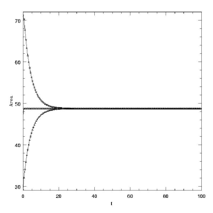
FIG. 1.: CMFT detection and tracking, in units of $M$, of a nonspinning $M=1$ black hole. Here area is given in units of $M^{2}$, and increasing $t$ (units of $M$) corresponds to propagation into the past.

In this section the accuracy of an implementation of the cmft method is considered in detail. For more detailed discussion of the signatures of black hole event horizons in the eikonal equation see [15] and [4]. Briefly, since the event horizon of a black hole is a global structure of spacetime, its detection cannot be determined without the complete history of the Cauchy evolution of the spacetime. However, as shown below, the horizon is a critical outgoing null surface that neither expands to infinity nor collapses into the gravitational singularity. Numerical event horizon solvers have typically employed this property as the signature behavior of event horizon detection and tracking. In these approaches, the space of outgoing null surfaces propagated into the past is surveyed for evidence of the critical behavior of the horizon. Since outgoing null data followed into the past tend to approach the horizon to great precision these methods typically produce highly accurate approximations of the event horizon itself. For example, in figure (1) we show outgoing data propagated into the past in a background spacetime contatining a spherically symmetric black hole. In that figure three classes of data are considered: Null data initially interior to the black hole event horizon, null data initially exterior to the black hole event horizon and null data that is exactly on the black hole event horizon. In all cases, we see that outgoing null data propagated into the past approaches the black hole event horizon to high accuracy.

FIG. 2.: CMFT detection and tracking, in units of $M$, of nonspinning black holes: $M=1/2,1,2$. Here increasing $t$ corresponds to propagation into the past.

To establish the accuracy of our implementation, we consider first the case of stationary, spinning black holes, which is completely described by the Kerr - Newmann axisymmetric solutions of Einstein’s equation. According to Carter’s theorem [24], this family of solutions is the unique, asymptotically flat, stationary and axisymmetric black hole solutions of the vacuum equations. As such, it is sufficient to consider this class of solutions in an account of stationary black hole event horizons. It is convenient to the discussion to make use of the Kerr-Schild form for the metric [25]:

$$g^{ab}=\eta^{ab}-2Hl^{a}l^{b}.$$ (13)

Here $\eta_{ab}=\mathrm{diag}\left(-1,1,1,1\right)$ is Minkowski’s metric, $H$ is a space time scalar, and $l^{a}$ is an ingoing null vector with respect to both the Minkowski and full metric. The Kerr solution is the two parameter family of solutions such that

$$H=\frac{Mr^{3}}{r^{2}+a^{2}z^{2}}$$ (14)

and

$$l^{t}=-1,$$ (15)

$$l^{x}=\frac{rx+ay}{r^{2}+a^{2}},$$ (16)

$$l^{y}=\frac{ry-ax}{r^{2}+a^{2}},$$ (17)

$$l^{z}=\frac{z}{r},$$ (18)

$$r^{2}=\frac{1}{2}\left(\rho^{2}-a^{2}\right)+\sqrt{\frac{1}{4}\left(\rho^{2}-a^{2}\right)+a^{2}z^{2}}$$ (19)

where

$$\rho^{2}=x^{2}+y^{2}+z^{2}.$$ (20)

FIG. 3.: CMFT analysis of $e$-folding time, in units of $M$, for nonspinning black holes of different masses. This figure shows pairs of interior and exterior data converging to the horizon, where the pairs are top to bottom $4M$, $2M$, and $M$. Here increasing $t$ corresponds to propagation into the past.

Two points are worth mentioning. Firstly, the parameter $M$ corresponds to the gravitational mass of the source, while the parameter $a$ corresponds to the source’s spin: It can be shown that observers at asymptotic infinity measure the angular momentum of the source to be $J=aM$. Secondly, the cartesian coordinates are chosen such that the $z$ axis is aligned with the direction of spin and so is an axis of symmetry.

FIG. 4.: CMFT tracking of spinning Black hole $a/M=0.25$.

The Kerr family of solutions is interesting from the perspective of tracking black hole event horizons since the solutions actually contain two event horizons; with one nested interior to the other. Furthermore, the solutions have a ring curvature singularity located at $r=z=0$. In the cmft method, provided the event horizon is approached from the exterior, neither of these features requires special attention.

FIG. 5.: CMFT tracking of spinning Black hole $a/M=0.5$

It is analytically known that the outermost horizon of a spinning black hole is located at the surface

$$r_{+}=M+\sqrt{M^{2}-a^{2}}$$ (21)

with an area

$$A=4\pi\left({r_{+}}^{2}+a^{2}\right).$$ (22)

We will now validate our cmft codes’ ability to determine these values.

FIG. 6.: CMFT tracking of spinning Black hole $a/M=0.75$

We start with nonspinning black holes. With $a=0$, figure (1) shows the signature of the black hole event horizon for outgoing null data propagated backwards in time. Figure (2) similarly shows this effect for outgoing data and includes variation in the mass with the cases of $M=1/2,1,2$ considered.

FIG. 7.: CMFT tracking of spinning Black hole $a/M=0.9$

In all cases interior and exterior data converge exponentially to the event horizon as predicted by the exact solution. The $e$ - folding time of this exponential behavior (which can be shown in perturbation theory to satisfy $\gamma=\left(4M\right)^{-1}$ for ingoing Eddington - Finkelstein coordinates) is shown numerically in figure (3). The slope of each line is $\left(4M\right)^{-1}M$ in agreement with the perturbation prediction.

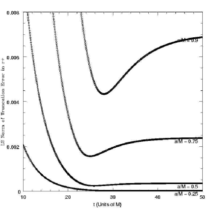
FIG. 8.: Scaling of truncation error, in units of $M$, of $r_{+}$ for a spinning Black hole $a/M=0.25$, $0.5$, $0.75$, $0.9$ using CMFT tracking. Here increasing $t$ corresponds to propagation into the past.

We turn now to consideration of spinning black holes. The ellipsoidal geometry of sections of spinning black hole event horizons are demonstrated in figures (4), (5), (6), (7), which show the intersection of the event horizon section both with a $\phi=\pi$ slice and with a $\theta=\pi/2$ slice. These figures are the asymptotic limit cross sections of spheres tracked backwards until the area achieves stationarity. They are thus approximations of the black hole event horizons. The figures are drawn for $a/M=0.25,0.5,0.75,$ and $0.9$. As can be seen there is a slight asymmetry (an error) of the resulting surfaces. The accuracy of these results is shown in figure (8), which contains the L2 norm of the numerical truncation error $e_{r}$ of the $r_{+}$ function calculated over the surface of the final state. With $\hat{r}_{+}$ denoting the finite difference approximation of the continuum funtion $r_{+}$, the truncation error is defined to be

$$e_{r}=\hat{r}_{+}-r_{+}.$$ (23)

In figure(8) time in units of $M$ is measured increasing into the past.

Figure (9) shows several values of the percent error in the area for a fixed unit mass black hole with spin parameter $0\leq a\leq 0.9$. These figures were generated using a numerical resolution of $m^{2}$ with $m=50$ on the detected event horizon surface section. The truncation error of the numerical integration of the area scales at least as well as ${\mathcal{O}}\left(h^{2}\right)$ as required for second order convergence. This scaling of the truncation error is shown in figure (10), which shows the percentage error of the area of a nonspinning black hole for resolutions of $m^{2}$ with $m=25,50,100$.

In terms of the consistency of these results for the truncation error of $r_{+}$ and the percent errors of the calculated areas, note that there are at least two sources of systematic error in the numerical calculation of the area of any surface. One source of error is the accuracy with which each point of the surface is known, while the second source of error is the finite resolution of the discrete version of the surface. Let $A$ denote the continuum area and $\hat{A}$ be the discrete version of the surface calculated using a resolution of $m^{2}$. Then by the finite difference approximation

$$A=\hat{A}+{\mathcal{O}}\left(1/m^{2}\right)$$ (24)

for second order convergence. However, if the points of the surface are systematically inaccurate $\hat{A}$ will not converge to $A$ in the continuum limit; instead $\hat{A}$ will converge to the bias of the implementation. This result suggests that the bias in $\hat{A}$ is on the order of $0.1$ percent.

The $e$-folding time for relaxation of outgoing null data onto the event horizon, or equivalently for formation of the solution singularity in the eikonal, is shown in figure (11) with various values of the spin $a/M=0.25,$ $0.5,$ $0.75,$ $0.9$. Note that only for the cases of rapidly spinning black holes $a/M\approx 0.9$ does the $e$-folding time differ appreciably from the spin zero case of $\gamma=1/4M$. These results suggest using the ‘rule of thumb’ relaxation time of $\gamma\approx 1/4M$ for any spin with $a/M\leq 0.9$.

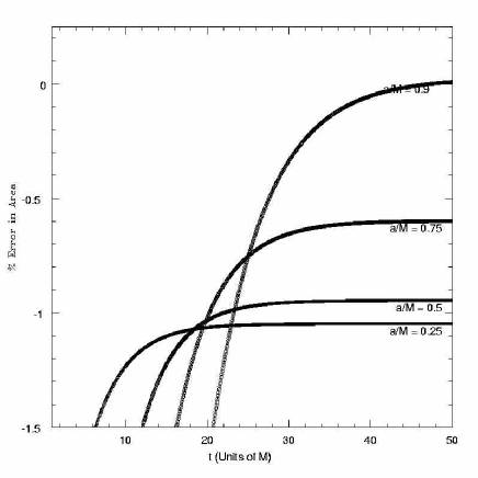
FIG. 9.: Percent error in area for spinning black hole $0<a/M<0.9$ using CMFT tracking. Here increasing $t$ corresponds to propagation into the past.

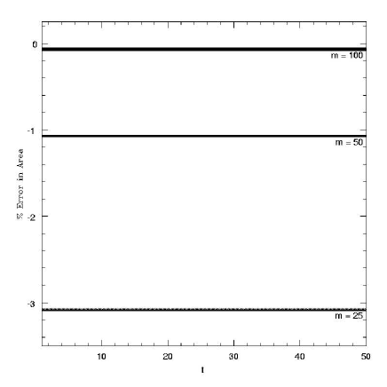
FIG. 10.: Scaling of truncation error in area for spin zero black hole with surface resolutions of $m^{2}$, with $m=25$, $50$, $100$. Here increasing $t$ corresponds to propagation into the past.

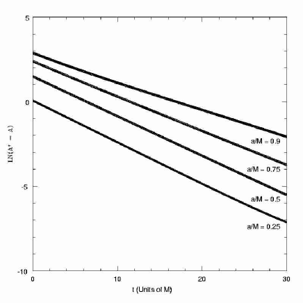
FIG. 11.: CMFT analysis of $e$-folding time, in units of $M$, for spinning black hole $0<a/M<0.9$. Here increasing $t$ corresponds to propagation into the past.

B Non-linear Coordinate Deformations

The method of comoving adaptive meshes makes use of an intricate numerical procedure: The passing and interpolation of data from one spherical grid to another. To ensure that the computational implementation of the method is both accurate and robust, consider the case of the following coordinate transformation:

$$t\rightarrow t^{\prime}=t,$$ (25)

$$x\rightarrow x^{\prime}=x+b\cos\omega t,$$ (26)

$$y\rightarrow y^{\prime}=y+b\sin\omega t,$$ (27)

$$z\rightarrow z^{\prime}=z$$ (28)

A nonspinning black hole located at $x=y=z=0$, is then seen to rotate with angular frequency $\omega$ at a radius of $r=b$ about the point $x^{\prime}=y^{\prime}=z^{\prime}=0$. The physics of this coordinate transformation is trivial and the area of the source event horizon remains $A=16\pi M^{2}$. However, from the perspective of the numerical implementation written in the coordinates $\left(t^{\prime},x^{\prime},y^{\prime},z^{\prime}\right)$, the black hole appears highly dynamical and moving with an angular velocity. As such, the coordinate transformation $\left(t,x,y,z\right)\rightarrow\left(t^{\prime},x^{\prime},y^{\prime},z^{\prime}\right)$ applied to the Kerr - Newmann family of analytic sources is a stringent test of an implementation of the method of comoving adaptive meshes.

Consider first the case of a linear shift of coordinates: $\omega=0,b\neq 0$. Figure (12) shows the percent error in the area of the detected horizon versus time increasing under propagation into the past, while figure (13) shows the L2 norm of the error in the function $r_{+}$ for $b=3/2,1,1/2,0$. Both of these figures are generated using surfaces of $m^{2}$ points with $m=25$ and spherical initial data of radius $r=2$ centered at the origin. The source is that of a nonspinning unit mass black hole. The solution ultimately settles down to the correct shift zero result, which suggests that this implementation of the method is stable with respect to translation of the source.

Additional complexity is obtained by fixing $b=1$ and varying $\omega=2\pi/T$. Figure (14) shows the percentage error in the area of the detected horizon section, while figure (15) shows the L2 norm of the error in $r_{+}$. In these figures the surface used was that of $m^{2}$ points with $m=25$, and spherical initial data of radius $r=3$ located at the origin. Also here, the source considered in both figures is a unit mass black hole with spin parameter $a=m/2$. According to these results, this implementation of the method of comoving adaptive meshes converges to the bias of the surface resolution as $\omega\rightarrow 0$. Further, for time scales on the order of the relaxation time $4M$, the error of the implementation is fairly significant although it remains below $10\%$. These result suggests that the particular implementation is sensitive to coupling of the time scale of the event horizon’s dynamics. Further accuracy can be obtained by considering a more stringent implementation.

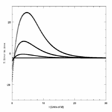
FIG. 12.: Percentage error in area of nonspinning black hole in shifted coordinates: $b=0,1/2,1,3/2$. Here increasing $t$ corresponds to propagation into the past.

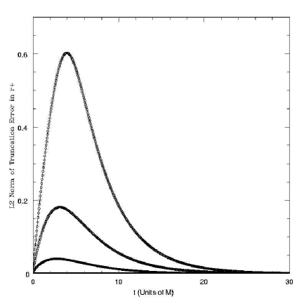
FIG. 13.: L2 norm of truncation error, in units of $M$, of $r_{+}$ for nonspinning black hole in shifted coordinates: $b=0$, $1/2$, $1$, $3/2$.Here increasing $t$ corresponds to propagation into the past.

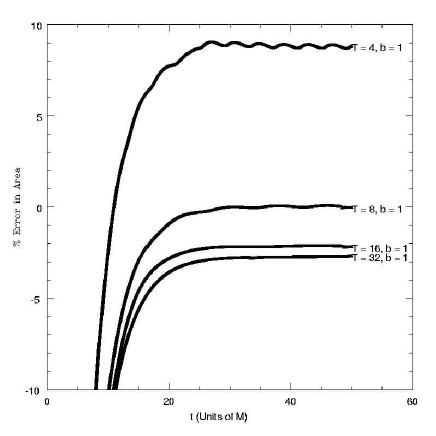
FIG. 14.: Percentage error in area of $a/M=1/2$ black hole in ‘wobbling’ coordinates : $b=1$, $\omega=2\pi/T=$ $\pi/2$, $\pi/4$, $\pi/8$, $\pi/16$. Here increasing $t$ corresponds to propagation into the past.

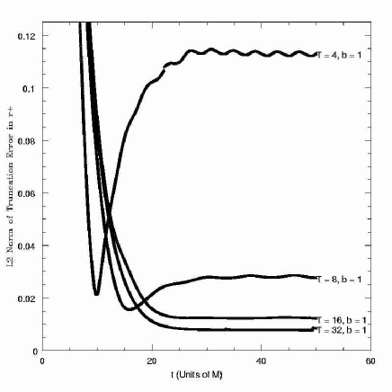
FIG. 15.: L2 norm of truncation error, in units of $M$, of $r_{+}$ for $a/M=1/2$ black hole in ‘wobbling’ coordinates : $b=1$, $\omega=2\pi/T$ $=\pi/2$, $\pi/4$, $\pi/8$, $\pi/16$. Here increasing $t$ corresponds to propagation into the past.

III Symmetric Binary Black Hole Coalescence

The cmft method cannot continuously monitor a topological transition in the event horizon of a black hole. However, with high resolution or refinement the method can detect the onset of a topological transition and come arbitrarily close to the transition itself.

In this context we now consider the Kastor - Traschen analytic solution of the Einstein - Maxwell $Q=M$ equations with cosmological constant $\Lambda=3H^{2}$ [19] [26]. The solution is simply

$$ds^{2}=-U^{-2}dt^{2}+U^{2}\left(dx^{2}+dy^{2}+dz^{2}\right)$$ (29)

where

$$U=-Ht+\frac{M_{1}}{r_{1}}+\frac{M_{2}}{r_{2}}.$$ (30)

$H=\pm\sqrt{\Lambda/3}$ and we set the coordinates and choose the sign so that $H=1$. These are the choices made in ref [29]. Both refs. [26] and [29] show that with these choices the black hole merger occurs in the future (i.e. as $t\equiv t\uparrow$ increases into the future). The sign convention differs between refs. [26] and [29]; we follow [29].

Here also, $M_{1}$ and $M_{2}$ denote the masses of the two holes located at $a_{1}$ and $a_{2}$ with

$$r_{1,2}=\sqrt{x^{2}+y^{2}+(z-a_{1,2})^{2}}.$$ (31)

FIG. 16.: Onset of topological transition in the Kastor Traschen solution using CMFT tracking as the event horizon is tracked backwards in time from the late time (outermost) horizon.

We consider the equal mass case ($M_{1}=M_{2}=0.1$), symmetrically oriented ($a_{1}=-a_{2}=a=0.1$) on the $z$-axis. These are the parameters chosen in a calculation by Siino[29]. The choice of relatively small $M$ keeps the final (postmerger) single black hole horizon inside the cosmological (deSitter) horizon. Ref. [26] demonstrates that for small negative $t$ there is one component of the event horizon that encompasses the origin; at somewhat earlier times there are two separated components of the event horizon. Figure 16 shows the cmft front tracker result (running backward from a late time t but still with $t<0$ ), with an “initial” guess equal to the late time single apparent horizon. Refs [26] and [29] estimate the late time single horizon at the apparent horizon:

$$r_{bh}=-R_{bh}/(Ht)=-(1-2MH-\alpha)/(2tH^{2}),$$ (32)

where

$$\alpha=\sqrt{1-4MH},$$ (33)

and this $M=M_{1}+M_{2}$. ($R_{bh}$ is a constant, though $r_{bh}$ is not.)

The coalescence occurs at a small negative time estimated in [26] as: $t^{*}\approx-R_{bh}/(2aH)<0$, which for our parameters is $t^{*}=-0.763932$. Following coalescence the merged black hole settles down to the final state of a charged black hole in a spacetime with cosmological constant. Figure (16) shows several frames of a movie indicating bifurcation of the black hole event horizon when tracked backwards in time from the outermost, guess surface at the latest time. Note that the solution will eventually break down when the grid function $u$ becomes multiple valued. Note also that near the bifurcation the solution exhibits multiple time scales. For example, away from the throat the solution appears quasi-stationary, while at the throat the solution is clearly dynamic.

As we investigate the behavior of the horizon found by cmft near breakdown, we can look for evidence of power law scaling of the topological transition. In analogy to the topological transitions found in the bifurcation (“pinch off”) of fluid droplets, such power law scaling would be expected in the neck of the event horizon at the point and time of merger, or “pinch on” [18] [28] (the opposite of “pinch off”). Using cylindrical coordinates, let $\rho$ denote the radius of the throat connecting the two black holes. By the axial symmetry of the solution, $\rho=\rho\left(z,\phi,t\right)=\rho\left(z,t\right)$. At the “pinch on” time, $t=t^{*}$, $\rho\left(0,t^{*}\right)=0$. If the solution exhibits power law scaling then

$$\rho=C\left(t-t^{*}\right)^{\gamma}$$ (34)

for times after the “pinch on”.

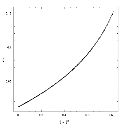
FIG. 17.: Throat radius $\rho$ versus $t-t^{*}$ just past the “pinch on” at $t=t^{*}$ in the Kastor-Traschen solution using CMFT tracking. Here increasing $t$ corresponds to propagation into the past. The $t$ used here increases into the future after the merger.

Figure (17) shows an order of magnitude in the evolution of $\rho$ just after the topological transition, using the cmft code. For $0.2\leq\left\|t-t^{*}\right\|\leq 0.6$ the radius of the throat appears to vary exponentially, while for $\left\|t-t^{*}\right\|\approx 0.0$ the radius appears to vary linearly. Figure (18) shows that behavior of $\rho$ is indeed purely exponential in $t$ far from the topological transition. Further, figure (19) (also found using the cmft code) shows evidence near the transition for power law (in fact, linear) scaling of the throat radius. Note that without arbitrarily high resolution or nested adaptive mesh refinement any scaling that is present in the solution cannot be resolved to machine epsilon. Therefore, the results presented here using the cmft code can at best establish qualitative evidence for such scaling. Figure (19) does indeed present such evidence that the solution exhibits power law scaling in analogy to the bifurcation of fluid droplets. Further, according to the results of the cmft code, it is here conjectured that the Kastor - Traschen solution scales like $\gamma\approx 1$. These results indicate that the cmft method is capable of probing into the fine structure of black hole event horizons undergoing a topological transition. Using the results from the cmft code, with $100^{2}$ points on the tracked surface, we obtain the computational estimate $t^{*}=-1.454.$

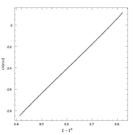
FIG. 18.: CMFT analysis of $e$ folding of the Kastor Traschen solution during the part of the evolution after, and away from the “pinch on”. The $t$ used here increases into the future after the merger.

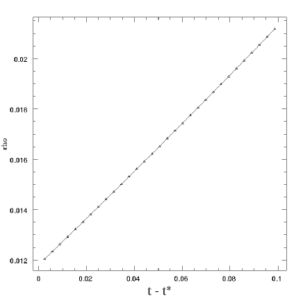
FIG. 19.: CMFT analysis of power law scaling at the topological transition of the Kastor Traschen solution after the “pinch on”. The $t$ used here increases into the future after the merger.

This result is somewhat different from the analytical estimates of Ref. [26]. However, we can verify this result because we can carry out a much more accurate direct (ordinary differential equation) integration to find the merge time. We use the equatorial symmetry of this equal mass case merger, for which the $\rho\approx t$ behavior is simply understood. In the equal mass case the throat is circular in cross section, and this cross section lies in the plane of symmetry of the problem. Suppose we introduce a cylindrical coordinate system for the metric (29). The event horizon is defined by outgoing null rays, and the throat thus is generated by null rays moving in the $\rho$ direction (the throat moves at the speed of light):

$$\frac{d\rho}{dt}=U^{-2}$$ (35)

where

$$U=Ht+2M/\sqrt{\rho^{2}+a^{2}}.$$ (36)

Figure (20) shows a log vs log plot of $\rho$ vs $t-t^{*}$, again begun from the late time single apparent horizon. It indicates a critical exponent of exactly $\gamma=1$. This plot was generated using an adaptive, Runge Kutta , numerical integration of the ordinary differential equation for $\rho\left(t\right)$ to drive the difference $t^{*}-t$ to below machine epsilon. The $t^{*}$ found in this simulation is $t^{*}=1.45845468374$, in agreement within accuracy to the cmft result.

Straightforward physics explains this answer. The instant of merger $t^{*}$ is not a special value for the Kastor - Traschen metric function $U$. Hence, near this event, equation (35) for $\rho$ is simply

$$\frac{d\rho}{dt}=U^{-2}\left(t^{*}\right)=\mathrm{const}\neq 0$$ (37)

plus higher order terms. Thus, in particular, the geometrically significant quantity, the circumference of the throat, $C(t)\approx U(t^{*})2\pi\rho(t)$ grows linearly with time, $\gamma=1$.

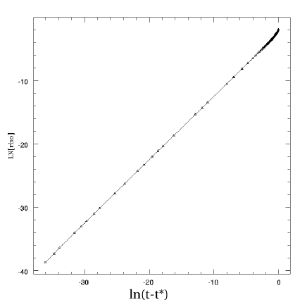
FIG. 20.: Power law scaling of topological transition in Kastor Traschen solution after the “pinch on”, computed using an adaptive Runge Kutta method. The $t$ used here increases into the future after the merger.

IV Conclusions

We have argued here that adaptive mesh refinement applied to the front tracking approach to tracking black hole event horizons is a potentially fruitful method; and moreover proves necessary for black hole processes in which the event horizon undergoes either a change of topology or develops creases or caustics. Towards that end we have developed an adaptive mesh technique that makes use of comoving meshes and demonstrated the accuracy of our approach. Applying our method to the symmetric collision data of the Kastor Traschen analytic solutions, we have found the surprising result of a power law in the minimal radius of the throat connecting the black holes following merger. We have shown power law scaling for the throat diameter at merger of black holes in a special situation: $\Lambda=3(\neq 0)$, $M_{1}=M_{2}=0.1$, $Q=M$, and axisymmetic. This effect is in analogy to that of fluid droplet problems. Since it is generically true that the black hole event horizon satisfies dynamical evolution equations that are exactly the form of a two dimensional fluid, we conjecture and give some qualitative arguments below concerning the specializations in the Kastor Traschen to argue that the power law scaling found in the Kastor Traschen solution must be generic for the symmetric collision of two black holes. Extending the analogy further, we also expect a similar power law for the asymmetric problem, although generalized in that case to accomodate the asymmetry of the problem as we now argue.

It is clear that $\Lambda\neq 0$ is irrelevant to this phenomena. The scaling behavior applies to an arbitrarily thin neck that first connects merging black holes. The curvature of the neck scales as $1/(\rho\times\mathrm{separation})\approx\left(\rho M\right)^{-1}$. For small $\rho M$ this dominates the fixed contribution.

The assumption of extremal black holes ($Q=M$) is a strong one. In Newtonian terms, it implies no acceleration of the motion between the holes (the electrical force is of equal magnitude and opposite the gravitational force). A first intuition may be that this has something to do with the exponent $\gamma$ in the scaling of the throat radius ($\gamma=1$ both numerically and analytically). However, the generic axisymmetric merger of black holes will deal with the scaling in a very brief interval at the beginning of merger; the “relative velocities” of the holes will be essentially constant in any case. We thus predict that extremality ($Q=M$) is not essential to the $\gamma=1$ power law behavior found here. For similar reasons we do not expect the spin of holes (zero in the case of the Kastor - Traschen solution) to affect the results found here. [The special (non-generic) case where non-extremal equal mass hole data are set with the holes just at merger will be different, because we expect the holes to “accelerate from zero” as the throat grows.]

Still in the context of axisymmetry, we can investigate whether the assumption of equal mass is relevant to the value of $\gamma$. In the limit of $M>>m$ we essentially consider a null topological tube (the small hole $m$) merging with a null plane $M$. We are investigating this configuration for merger. We again expect power law scaling; the question is to determine the exponent. If in this case $\gamma\neq 1$, then $\gamma$ will in general be a function of the ratio of the masses: $\gamma=\gamma(m/M)$; $\gamma(1)=1$. We no longer have the symmetry plane to simplify analysis; the throat cannot be followed by following the individual $\rho$ direction null trajectories, but Lindblom [30] has given an argument, based on the smoothness of the throat after its formation, that gives $\gamma=1$ for the growth of the circumference in this case also.

Finally, we consider relaxing axisymmetry. In analysis and simulations based on perturbation of late time horizons evolved backwards[11], toroidal behavior is sometimes seen in the non-axisymmetric case. The horizons grow more then one “point” as they approach merger; two points that touch simultaneously in very quick succession will create an evanescent toroidal horizon. To date, there has been no study directly relating parameters of the toroid to parameters of the colliding holes (we have seen only suggestions of toroidal behavior in any of our computations (c.f. the “offset points” of the event horizon in [31], Figure 11) , perhaps because of resolution limitations). However, we would expect each merging “point” to behave like a seperate merger and thus to undergo power law scaling, but not necessarily with $\gamma=1$. In fact, analysis by Winicour [11] in the generic case shows that the toroid closes superluminally; thus prevents sending signals “through the hole”. This requires that the “points” grow superluminally, which requires $\gamma<1$. The crucial difference from the case explained by Lindblom, is that the toroidal structure is not described by a smooth surface. In particular, there is an inner “crease” where geodesics are joining the torus, allowing it to close superluminally.

V Ackmowledgment

We thank L. Lindblom for very insightful and helpful comments. This work was supported by NSF rant PHY0102204. Computations were done at the University of Texas Advanced Computing Center.

REFERENCES

- [1] S.A. Hughes et al, Phys. Rev D., 49, 4004 (1994).
- [2] P. Anninos et al, Phys. Rev Lett., 74, 630 (1995).
- [3] R. A. Matzner et al, Science, 270, 941 (1995).
- [4] J. Libson et al, Phys. Rev. D., 53, 4335 (1996).
- [5] Misner, K. S. Thorne, C. W. and J. A. Wheeler, “Gravitation”, Freeman (1973).
- [6] S. L. Shapiro, S. A. Teukolsky, and J. Winicour, Phys. Rev D., 52, 6982 (1995).
- [7] T. Jacobson and S. Venkataramani, Class. Quant. Grav., 12, 1055 (1995).
- [8] P. T. Chrusciel and R. M. Wald, Class. Quant. Grav., 11, 147 (1994).
- [9] M. Siino, Phys. Rev. D., 58, 104016 (1998).
- [10] M. Siino, Phys. Rev. D., 59, 64006 (1999).
- [11] S. Husa and J. Winicour, Phys. Rev D., 60, 84019 (1999).
- [12] P. T. Chrusciel and G. J. Galloway, Commun. Math. Phys., 193, 449 (1998).
- [13] Chrusciel et al, P. T., Annales Henri Poincare, 2, 109 (2001).
- [14] Chrusciel et al, P. T., Journal Geom. Phys, in press, (2001)
- [15] S. A. Caveny, M. Anderson and R. A. Matzner, In press (2002).
- [16] R. H. Price and K. S. Thorne, Phys. Rev. D., 33, 915 (1986).
- [17] J. Masso et al, Phys. Rev. D., 59, (1999).
- [18] J. Eggers, Phys. Rev. Lett., 71, 3458 (1993).
- [19] D. Kastor and J. Traschen, Phys. Rev. D., 47, 4476 (1993).
- [20] M. Berger and J. Oliger, J. Comp. Phys., 53, 484 (1984).
- [21] M. W. Choptuik, Phys. Rev. Lett., 70, 9 (1993).
- [22] Bishop et al, N. T., “Approaches to Numerical Relativity”, Cambridge University Press (1992).
- [23] S. A. Teukolsky, Phys. Rev. D, 61, 087501 (2000).
- [24] B. Carter, Phys. Rev. Lett., 26, 331 (1971).
- [25] D. M. Shoemaker, M. F. Huq, and R. A. Matzner, Phys. Rev. D, 62, 124005 (2000).
- [26] D. Brill et al, Phys. Rev. D., 49, 840 (1994).
- [27] T. W. Baumgarte et al, Phys. Rev. D., 54, 4849 (1996).
- [28] Goldstein et al, R. E., Phys. Rev. Lett., 70, 3043 (1993).
- [29] Masaru Siino, “Topological Appearnce of Event Horizon” Prog. Theor. Phys. 99, 1 (1998) [gr-qc 98 03099].
- [30] L. Lindblom, private communication (2003).
- [31] Scott A. Caveny, Matthew Anderson, and Richard A. Matzner, “Tracking Black Holes in Numerical Relativity”, submitted to Phys. Rev D (2003) [gr-qc/0303099].