A Quantum Weak Energy Inequality for Spin-One Fields in Curved Spacetime

Abstract

Quantum weak energy inequalities (QWEI) provide state-independent lower bounds on averages of the renormalised energy density of a quantum field. We derive QWEIs for the electromagnetic and massive spin-one fields in globally hyperbolic spacetimes whose Cauchy surfaces are compact and have trivial first homology group. These inequalities provide lower bounds on weighted averages of the renormalized energy density as “measured” along an arbitrary timelike trajectory, and are valid for arbitrary Hadamard states of the spin-one fields. The QWEI bound takes a particularly simple form for averaging along static trajectories in ultrastatic spacetimes; as specific examples we consider Minkowski space [in which case the topological restrictions may be dispensed with] and the static Einstein universe.

A significant part of the paper is devoted to the definition and properties of Hadamard states of spin-one fields in curved spacetimes, particularly with regard to their microlocal behaviour.

I Introduction

In common with all observed forms of classical matter, the spin-one fields described by the Maxwell and Proca equations obey the weak energy condition (WEC). That is, the stress-energy tensor $T_{ab}$ obeys $T_{ab}v^{a}v^{b}\geq 0$ for all timelike vectors $v^{a}$. In classical general relativity, energy conditions such as the WEC play a key role in many important results, notably the singularity theorems of Penrose Penrose (1965) and Hawking Hawking (1965). Moreover, since any metric solves the Einstein equations for some choice of stress-energy tensor, it is arguable that general relativity has limited predictive power in the absence of such conditions.

However, all classical energy conditions are violated by quantum fields, as has been known for many years Epstein et al. (1965). Typically, the energy density at a given spacetime point is unbounded from below as a function of the state. Specific examples of negative energy states are provided by highly squeezed states of light in quantum optics, the Casimir vacuum state for a quantized field between uncharged perfectly conducting parallel planar plates and the Boulware vacuum state outside a black holes. Replacing the classical stress-energy tensor on the right hand side of Einstein’s equation with its quantum expectation value, we must therefore allow for negative energy sources, raising the possibility of exotic phenomena within the realm of semiclassical gravity. For example, negative energy can be used to maintain static traversable wormholes Morris and Thorne (1988); Morris et al. (1988), create naked singularities Hiscock (1981); Ford and Roman (1992), travel faster than light Alcubierre (1994); Krasnikov (1998), and travel backward through time Morris et al. (1988); Everett (1996). In negative energy models studied by Parker and Fulling it is even possible to avoid the cosmological singularity Parker and Fulling (1973), thus threatening to overthrow the classical singularity theorems. One might also expect that negative energy fluxes could lead to macroscopic violations of the second law of thermodynamics Ford (1978).

Of course, macroscopic violations of the second law are not observed in nature. Motivated by these thermodynamic considerations, Ford Ford (1978) deduced that the negative fluxes and energy densities of quantum fields must be subject to constraints, at least on average. These constraints, known as quantum inequalities, or QI, provide state-independent lower bounds on certain weighted averages of the stress-energy tensor. They may therefore be regarded as the remnants of the classical energy conditions after quantisation; thus, for example, the analogue of the WEC is sometimes referred to as a quantum weak energy inequality or QWEI. Such bounds typically take the form

$$\int\langle:T_{ab}(\gamma(\tau))u^{a}(\tau)u^{b}(\tau):\rangle_{\omega}\,f(\tau)\,d\tau\geq-{\mathfrak{Q}}(\gamma,f)\,,$$ (1)

where $f\geq 0$ is the weight, or sampling function, $\gamma$ is a smooth timelike curve, parametrised by proper time $\tau$ and with four-velocity $u^{a}=(d\gamma/d\tau)^{a}$, and $:T_{ab}:$ denotes the stress-energy tensor, normal ordered with respect to some reference state $\omega_{0}$. The significant point is that the bound ${\mathfrak{Q}}(\gamma,f)$ is independent of the state $\omega$. The class of states $\omega$ for which the bound holds must also be delineated—all bounds in the literature require (at least) that $\omega$ and $\omega_{0}$ be Hadamard states, although this can be weakened slightly. Of course the normal ordered energy density differs from the renormalised energy density by the (renormalised) energy density of the reference state. Accordingly, Eq. (1) may easily be converted into a bound on the renormalised energy density.

As we will shortly describe, various authors have established QWEI’s for the scalar and Dirac fields in different circumstances, leading up to general results valid in curved spacetimes. The main aim of the present paper is to establish similar QWEI’s for the Maxwell and Proca fields in general globally hyperbolic spacetimes. In order to do this, we have also made a detailed study of the field theories concerned, particularly in relation to the class of Hadamard states. Several new results obtained here may therefore be of more general interest.

As already mentioned, the earliest work on quantum inequalities is due to Ford, who established a bound on negative energy fluxes for scalar fields in 1991 Ford (1991). The first QWEI was obtained for the massless, minimally-coupled scalar field in Minkowski spacetime by Ford and Roman Ford and Roman (1995), who established the inequality (1) for the case of an inertial worldline $\gamma$ and with $f$ taking the Lorentzian form $f(\tau)=\tau_{0}/(\pi(\tau^{2}+\tau_{0}^{2}))$, in which $\tau_{0}$ sets the characteristic timescale for the averaging. In four dimensions, the resulting bound was

$$\int\langle:T_{ab}(\tau)u^{a}(\tau)u^{b}(\tau):\rangle_{\omega}\,\frac{\tau_{0}}{\pi(\tau^{2}+\tau_{0}^{2})}\,d\tau\geq-\frac{3}{32\pi^{2}\tau_{0}^{4}}\,.$$ (2)

These results were then extended by Ford and Roman to the massive scalar field in Minkowski space Ford and Roman (1995, 1997) and were further extended by Pfenning and Ford to minimally-coupled scalar fields of arbitrary mass in ultrastatic curved spacetimes Pfenning and Ford (1997, 1998); Pfenning (1998). In these generalisations, it was found that the dominant term of the QWEI has a form similar to Eq. (2), but with subdominant correction terms due to the curvature and the mass of the field. Pfenning and Ford also showed that one could express the bound on the right hand side of the QWEI in terms of derivatives of the Euclidean Green’s function for the spacetime and developed a short sampling time approximation to the QWEI which could be used in spacetimes where it would be too hard to calculate the exact QWEI bound.

The restriction to the Lorentzian weight $\tau_{0}/(\pi(\tau^{2}+\tau_{0}^{2}))$ was removed by various authors. By making use of the conformal properties of field theories in two dimensions, Flanagan Flanagan (1997, 2002) has derived optimal quantum inequalities for the massless scalar field for arbitrary smooth positive sampling functions, and Vollick has done the same for the Dirac field Vollick (2000). QWEI’s for the minimally coupled scalar field in static curved spacetimes of any dimension for an arbitrary sampling function were established by Fewster in work with Eveson Fewster and Eveson (1998) and Teo Fewster and Teo (1999).

More recently, techniques drawn from microlocal analysis have been used to considerably generalise previous QWEI’s and to put them on a mathematically rigorous footing. Fewster Fewster (2000) used these techniques to derive a QWEI for minimally coupled scalar fields in general globally hyperbolic spacetimes (the most general class on which the Klein–Gordon equation is well-posed). In this case, averaging takes place along an arbitrary timelike worldline, using any weight of the form $f(t)=g(t)^{2}$ for $g$ smooth, real-valued and compactly supported. Subsequently, Fewster and Verch established similar results for the Dirac and Majorana fields in four-dimensional globally hyperbolic spacetimes Fewster and Verch (2002). Averaging over spacetime volumes has been considered by Helfer Helfer , also in great generality.

Previous work on QWEIs for spin-one fields has focussed on the electromagnetic field, beginning with the work of Ford and Roman Ford and Roman (1997), who derived a QWEI for the case of Lorentzian sampling along inertial trajectories in Minkowski space. More recently, Pfenning Pfenning (2002) has derived a QWEI for the electromagnetic field in static curved spacetimes with arbitrary positive weight sampling functions by using the techniques developed for the scalar field in Fewster and Eveson (1998); Fewster and Teo (1999). Using similar techniques, Marecki Marecki (2002) has derived bounds on the fluctuations of the electric field strength, which are of interest in quantum optics.

In this paper we will adapt the methods of Fewster (2000) to the Maxwell and Proca fields. This depends crucially on the fact, first discovered by Radzikowski Radzikowski (1996) for scalar fields, that the class of Hadamard states may be characterised in terms of a wave-front set condition on the two-point function. Similar reformulations are known for the Dirac field Kratzert (2000); Hollands (2001); Sahlmann and Verch (2001) but there is as yet no full treatment for the Maxwell and Proca fields in the literature. (See, however, Brown and Ottewill (1986); Allen and Ottewill (1992) for [non-microlocal] discussions of Hadamard states for electromagnetism using Faddeev–Popov ghosts.) Our treatment of this issue has been influenced to some extent by the forthcoming work of Junker and Lledó Junker and Lledó , although it has been conducted largely independently, leading to some technical differences with their approach .

The paper is structured as follows. The Maxwell and Proca fields are most elegantly described using differential forms; accordingly, we begin in Section II with a description of our conventions for differential forms and other geometric objects which will appear in this paper. In particular, we delineate the class of globally hyperbolic spacetimes to be considered; for technical reasons it is convenient to assume that their Cauchy surfaces are compact and have trivial first homology group. This is followed by a brief introduction to microlocal analysis leading to the definition of the wave-front set for $p$-form distributions.

In Sec. III we describe the quantisation of the Maxwell and Proca fields in globally hyperbolic spacetimes. We adopt an algebraic approach, giving a direct construction of algebras of observables equivalent to those obtained by Dimock Dimock (1992) and Furlani Furlani (1999). We also define the notion of a Hadamard state for these fields, as a state whose two-point function  is related in a certain way to a one-form Klein–Gordon bisolution of Hadamard form. Such bisolutions and their microlocal properties have been discussed in detail by Sahlmann and Verch Sahlmann and Verch (2001); we may therefore read off the microlocal properties of the Maxwell and Proca two-point functions in Hadamard states. This permits us to apply the methods of Fewster (2000) to obtain quantum inequalities for these fields in Sec. V. Before this, in Sec. IV, we specialise to the class of ultrastatic spacetimes in order to gain further insight into the abstract definitions of Sec. III. In particular, we prove the existence of Hadamard states in these spacetimes and use deformation arguments Fulling et al. (1981) to deduce from this the existence of Hadamard states in general globally hyperbolic spacetimes obeying our topological restrictions. We also compare our approach with other quantisation schemes, including the Gupta–Bleuler method. As mentioned above, we expect that some of the results obtained here to be of wider interest.

In Sec. VI we investigate our QWEI in Minkowski space, and in general ultrastatic spacetimes (modulo the usual topological conditions). Simple formulae are obtained for the QWEI bound, which are readily compared with those previously obtained for the scalar field. In Minkowski space, the QWEI bound is weaker by a factor of exactly two for the Maxwell field (as already noted in Pfenning (2002)) and by a factor of three for the Proca field. This is not very surprising and simply reflects the number of spin degrees of freedom. In curved spacetime, however, the spin-one and scalar QWEIs cannot be related in this fashion. To emphasise this, we explicitly determine the QWEI bound in the Einstein static universe, providing a concrete example of our ultrastatic QWEI. Two appendices contain the proofs of some technical results required in the body of the paper.

II Preliminaries

Units where $\hbar=c=1$ are used throughout. The notation $C_{0}^{\infty}(\mathbb{R}^{n})$ denotes the space of smooth, compactly supported , complex-valued functions on $\mathbb{R}^{n}$.

II.1 Geometry and forms

Spin-one fields on globally hyperbolic spacetimes are most elegantly formulated in terms of differential forms. We will follow the conventions of Abraham et al. (1988), which we now briefly summarise for the benefit of the reader.

Suppose $\mathcal{N}$ is a smooth $n$-dimensional manifold which is connected, boundaryless, orientable, Hausdorff, paracompact, and equipped with a smooth metric of index $s$ . We denote the space of smooth, complex-valued $p$-forms on $\mathcal{N}$ by $\Omega^{p}(\mathcal{N})$; the subspace of compactly supported $p$-forms will be written $\Omega_{0}^{p}(\mathcal{N})$. Each $p$-form may be regarded as an antisymmetric covariant $p$-tensor field and we will occasionally use index notation accordingly. Thus the exterior product $\alpha\wedge\beta\in\Omega^{p+q}(\mathcal{N})$ of $\alpha\in\Omega^{p}(\mathcal{N})$ and $\beta\in\Omega^{q}(\mathcal{N})$ is given by

$$(\alpha\wedge\beta)_{a_{1}\cdots a_{p+q}}=\frac{(p+q)!}{p!q!}\alpha_{[a_{1}\cdots a_{p}}\beta_{a_{p+1}\cdots a_{p+q}]}\,,$$ (3)

and the exterior derivative ${\bf d}:\Omega^{p}(\mathcal{N})\to\Omega^{p+1}(\mathcal{N})$ is defined by

$$({\bf d}\alpha)_{a_{1}\cdots a_{p+1}}=(p+1)\nabla_{[a_{1}}\alpha_{a_{2}\cdots a_{p+1}]}\,,$$ (4)

where the square brackets denote antisymmetrisation and $\nabla_{a}$ is any connection on $\mathcal{N}$ (${\bf d}$ is independent of the choice of connection). The Hodge $*$-operator is defined uniquely as the map $*:\Omega^{p}(\mathcal{N})\to\Omega^{n-p}(\mathcal{N})$ such that

$$\alpha\wedge*\beta=\frac{1}{p!}\alpha_{a_{1}\ldots a_{p}}\beta^{a_{1}\cdots a_{p}}d{\rm vol}_{g}\,,$$ (5)

where $d{\rm vol}_{g}$ is the positive volume $n$-form associated with the metric $g$. In particular, $(*)^{2}=(-1)^{p(n-p)+s}$ on $p$-forms. By combining the Hodge $*$ and exterior derivative, we may define the coderivative $\bm{\delta}:\Omega^{p}(\mathcal{N})\to\Omega^{p-1}(\mathcal{N})$ (with the convention that $\bm{\delta}$ annihilates all zero-forms) by $\bm{\delta}=(-1)^{n(p-1)+s+1}*{\bf d}*$, which reduces to $\bm{\delta}=*{\bf d}*$ in a four-dimensional Lorentzian spacetime.

The operations introduced above allow us to define a symmetric pairing $\langle\cdot,\cdot\rangle$ of $p$-forms under integration: we set

$$\langle\mathcal{U},\mathcal{V}\rangle\equiv\int_{\mathcal{N}}\mathcal{U}\wedge*\mathcal{V}$$ (6)

for any $\mathcal{U},\mathcal{V}\in\Omega^{p}(\mathcal{N})$ for which the integral exists. Since ${\bf d}(\mathcal{U}\wedge*\mathcal{V})={\bf d}\mathcal{U}\wedge*\mathcal{V}-\mathcal{U}\wedge*\delta\mathcal{V}$, Stokes’ theorem gives

$$\langle\bm{\delta}\mathcal{U},\mathcal{V}\rangle=\langle\mathcal{U},{\bf d}\mathcal{V}\rangle$$ (7)

for smooth $(p+1)$- and $p$-forms $\mathcal{U}$ and $\mathcal{V}$ whose supports have compact intersection. In this sense the operators ${\bf d}$ and $\bm{\delta}$ are dual.

The Laplace-Beltrami operator is defined as $-({\bf d}\bm{\delta}+\bm{\delta}{\bf d})$, i.e., it is equal to minus the Laplace–de Rahm operator ${\bf d}\bm{\delta}+\bm{\delta}{\bf d}$. Where the manifold $\mathcal{N}$ is a Lorentzian spacetime, with signature $+-\cdots-$, the Laplace-Beltrami operator is also known as the D’Alembertian and will be denoted by $\Box$. We wish to point out that Dimock Dimock (1992) uses $\Box$ to denote the Laplace–de Rahm operator; our usage is determined by the convention that $\Box$ should have principal part $g^{\mu\nu}\partial_{\mu}\partial_{\nu}$, in accordance with typical usage in general relativity.

Finally, the spaces $\Omega_{0}^{p}(\mathcal{N})$ may be given locally convex topologies  and the corresponding topological duals $\Omega_{0}^{p}(\mathcal{N})^{\prime}$ will be called the spaces of $p$-form distributions on $\mathcal{N}$. (The pairing $\langle\cdot,\cdot\rangle$ provides a natural embedding of $\Omega^{p}(\mathcal{N})$ in $\Omega_{0}^{p}(\mathcal{N})^{\prime}$.) In the case $p=0$, we will also use $\mathcal{D}(\mathcal{N})$ and $\mathcal{D}^{\prime}(\mathcal{N})$ for $\Omega_{0}^{0}(\mathcal{N})$ and $\Omega_{0}^{0}(\mathcal{N})^{\prime}$ respectively. The exterior derivative and coderivative are defined on these spaces by

$$({\bf d}\mathcal{U})(f)=\mathcal{U}(\bm{\delta}f)\qquad(\mathcal{U}\in\Omega_{0}^{p}(\mathcal{N})^{\prime},~{}f\in\Omega_{0}^{p+1}(\mathcal{N}))$$ (8)

and

$$(\bm{\delta}\mathcal{U})(f)=\mathcal{U}({\bf d}f)\qquad(\mathcal{U}\in\Omega_{0}^{p}(\mathcal{N})^{\prime},~{}f\in\Omega_{0}^{p-1}(\mathcal{N}))$$ (9)

which extend the definitions given for smooth forms by virtue of the embeddings defined above and the calculation (7). In a similar way, the Hodge $*$-operator may also be extended to a map from $p$-form distributions to $(n-p)$-form distributions by

$$(*\mathcal{U})(f)=(-1)^{p(n-p)}\mathcal{U}(*f)\qquad(\mathcal{U}\in\Omega_{0}^{p}(\mathcal{N})^{\prime},~{}f\in\Omega_{0}^{n-p}(\mathcal{N}))\,;$$ (10)

and it is easily checked that the formula $\bm{\delta}=(-1)^{n(p-1)+s+1}*{\bf d}*$ remains true for distributions.

II.2 Microlocal analysis and the wave-front set

Our proof of the quantum weak energy inequality turns on the detailed singularity properties of various distributions related to the two-point functions of quantum fields in Hadamard states. The information required is encoded in the wave-front set of these distributions, which is defined as follows. (See Ref. Hörmander (1983) for a full presentation.)

We will define the Fourier transform $\widehat{u}$ of $u\in C_{0}^{\infty}(\mathbb{R}^{n})$ using the nonstandard convention

$$\widehat{u}(k)=\int d^{n}y\ u(y)e^{ik\cdot y},$$ (11)

which conforms to the conventions used e.g., in Fewster (2000). The Fourier transform can be extended to scalar distributions of compact support by writing $\widehat{u}(k)=u(f_{k})$ where $f_{k}=e^{ik\cdot y}$. Given a cone $V\subset(\mathbb{R}^{n}\backslash\{0\})$, we will say that $\widehat{u}(k)$ is of rapid decrease in $V$ if for each $N\in\mathbb{N}$ there exists a real constant $C_{N}$ such that

$$\left|\widehat{u}(k)\right|\leq\frac{C_{N}}{(1+|k|)^{N}}\qquad\forall\ k\in V,$$ (12)

where $|k|$ denotes the Euclidean norm of $k$.

Smooth compactly supported functions have Fourier transforms which decay faster than any inverse power in the whole of $\mathbb{R}^{n}$, but the same is not true for arbitrary distributions $u$ of compact support. A well known example is the Dirac $\delta$-function, whose Fourier transform does not decay at infinity in any direction. We define the set of singular directions $\Sigma(u)$ to be the set of all $k\in\mathbb{R}^{n}\backslash\{0\}$ having no conical neighbourhood $V$ in which $\widehat{u}$ is of rapid decrease.

More detailed information about the singularities of $u$ can be gained by localizing the singular directions. In particular, the set of singular directions of $u$ at a point $x$ is defined by

$$\Sigma_{x}(u)=\bigcap_{\chi}\Sigma(\chi u)\,,$$ (13)

where the intersection is taken over all smooth compactly supported test functions $\chi\in C^{\infty}_{0}(\mathbb{R}^{n})$ with $\chi(x)\neq 0$. The wave-front set ${\rm WF}\,(u)$ of $u$ is then defined by

$${\rm WF}\,(u)=\{(x,k)\in\mathbb{R}^{n}\times(\mathbb{R}^{n}\backslash\{0\})\ |\ k\in\Sigma_{x}(u)\}.$$ (14)

The wave-front set can be extended in a natural way to distributions on manifolds. Let $(\mathcal{N},g)$ be a smooth $n$-dimensional manifold of the type discussed above. Each distribution $u$ in $\mathcal{D}^{\prime}(\mathcal{N})$ has a representative $u_{\kappa}\in\mathcal{D}^{\prime}(\mathbb{R}^{n})$ in each coordinate chart $(U,\kappa)$ (with corresponding coordinates denoted $x^{\mu}=\kappa(x)^{\mu}$) defined so that

$$u_{\kappa}(f\sqrt{-|g|})=u(f\circ\kappa)$$ (15)

holds for every smooth function $f$ compactly supported in $\kappa(U)\subset\mathbb{R}^{n}$, where $|g|$ is the determinant of $g_{\mu\nu}$. The wave-front set ${\rm WF}\,(u)$ is now a subset of the cotangent bundle $T^{*}\mathcal{N}$ with the property that $(x,k)\in{\rm WF}\,(u)$ if and only if there is a chart $(U,\kappa)$ about $x$ so that $(\underline{x},\underline{k})\in{\rm WF}\,(u_{\kappa})$, where $(\underline{x},\underline{k})$ are the coordinates of $(x,k)$ and $u_{\kappa}$ is defined as in (15). In fact, it may be shown (see Theorem 8.2.4 and the following discussion in Ref. Hörmander (1983)) that the restriction of ${\rm WF}\,(u)$ to $U$ is given by

$${\rm WF}\,(u)\cap T^{*}U = \kappa^{*}{\rm WF}\,(u_{\kappa})$$ (16)

$$:= \{\kappa^{*}(\underline{x},\underline{k}):(\underline{x},\underline{k})\in{\rm WF}\,(u_{\kappa})\}\,,$$

where the pull-back $\kappa^{*}$ relates $(x,k)\in T^{*}\mathcal{N}$ to its coordinates by $\kappa^{*}(\underline{x},\underline{k})=(x,k)$.

There is a natural extension of the wavefront set to $p$-form distributions. Let $v_{i}$ $(i=0,\ldots,n-1)$ be a global orthonormal $n$-bein on $\mathcal{N}$ (i.e., the vectors $v_{i}$ obey $g_{ab}v_{i}^{a}v_{j}^{b}=\eta^{ij}$ and thus $\eta^{ij}v_{i}^{a}v_{j}^{b}=g^{ab}$, where $\eta^{ij}$ is diagonal with $s$ entries equal to $-1$ and the rest equal to $+1$) and let $V^{i}$ be the dual basis of one-forms: $V^{i}_{a}=\eta^{ij}g_{ab}v^{b}_{j}$. For each $\mathcal{U}\in\Omega_{0}^{p}(\mathcal{N})^{\prime}$, we may define the component distributions $\mathcal{U}_{i_{1}\cdots i_{p}}\in\mathcal{D}^{\prime}(\mathcal{N})$ by

$$\mathcal{U}_{i_{1}\cdots i_{p}}(f)=\eta_{i_{1}j_{1}}\cdots\eta_{i_{p}j_{p}}\mathcal{U}(fV^{j_{1}}\wedge\cdots\wedge V^{j_{p}})$$ (17)

for $f\in\mathcal{D}(\mathcal{N})$. Then we define the wave-front set of $\mathcal{U}$ to be

$${\rm WF}\,(\mathcal{U})=\bigcup_{i_{1},\dots,i_{p}}{\rm WF}\,(\mathcal{U}_{i_{1}\dots i_{p}})\,,$$ (18)

which may be shown to be independent of the particular choice of $n$-bein $v_{i}$.

III Quantisation of the Maxwell and Proca fields

III.1 Classical theory

We will consider the Maxwell and Proca fields propagating on four-dimensional Lorentzian globally hyperbolic spacetimes. Each such spacetime is a pair $(\mathcal{M},g)$ consisting of a four-dimensional, smooth, real manifold $\mathcal{M}$, with the topological properties listed at the start of Sec. II.1, together with a smooth Lorentzian metric $g$ with signature $(+,-,-,-)$. Global hyperbolicity, which will ensure well-posedness of our field equations, requires that $(\mathcal{M},g)$ be time-orientable and that $\mathcal{M}$ contain a Cauchy surface $\Sigma$, that is, a smooth spacelike hypersurface intersected precisely once by every inextendible causal curve in $\mathcal{M}$. In fact, one may show Dieckmann (1988) that $\mathcal{M}$ is diffeomorphic to $\mathbb{R}\times\Sigma$. We will assume for the most part that $\Sigma$ [also referred to as the spatial section] is compact and that $\Sigma$ has trivial first singular homology group with real coefficients, $H_{1}(\Sigma)$. This is equivalent to the triviality of the compact support de Rahm cohomology group $H_{c}^{3}(\mathcal{M})$ ; note that this condition excludes, for example, the 3-torus $T^{3}$ as a spatial section. The compactness assumption is made for convenience only; triviality of $H_{1}(\Sigma)$ is inessential for the Proca field, but appears to be required in order to establish some of our results for the Maxwell field.

The classical uncharged spin-$1$ field of mass $M>0$ is a real one-form field $\mathcal{A}\in\Omega^{1}(\mathcal{M})$ obeying the Proca equation

$$\left(-\bm{\delta}{\bf d}+M^{2}\right)\mathcal{A}=0\,.$$ (19)

Applying the coderivative $\bm{\delta}$ we see that $\bm{\delta}\mathcal{A}=0$ and so any solution to Eq. (19) also satisfies the one-form Klein–Gordon equation

$$\left(\Box+M^{2}\right)\mathcal{A}=0\,.$$ (20)

Conversely, any solution to (20) satisfying the constraint

$$\bm{\delta}\mathcal{A}=0$$ (21)

solves the Proca equation. The advantage of the system (20,21) is that (20) has the hyperbolic principal part $g^{\alpha\beta}\partial_{\alpha}\partial_{\beta}$ in local coordinates and therefore admits unique fundamental solutions $E^{\pm}_{M}:\Omega^{1}_{0}(\mathcal{M})\rightarrow\Omega^{1}(\mathcal{M})$ respectively Choquet-Bruhat (1968); Furlani (1999), such that

$$\left(\Box+M^{2}\right)E^{\pm}_{M}=E^{\pm}_{M}\left(\Box+M^{2}\right)=\openone$$ (22)

and ${\rm supp}\,(E^{\pm}_{M}\mathcal{J})\subset J^{\pm}({\rm supp}\,\mathcal{J})$ for $\mathcal{J}\in\Omega^{1}_{0}(\mathcal{M})$. Here, $J^{\pm}(S)$, the causal future($+$)/past($-$) of $S$, is defined to be the set of points in $(\mathcal{M},g)$ that can be reached from the set $S\subset\mathcal{M}$ by a future($+$)/past($-$) directed causal curve. The operators $E^{\pm}_{M}$ extend to $\mathcal{J}$ with ${\rm supp}\,\mathcal{J}$ compact to the past/future and for such $\mathcal{J}$, $\mathcal{A}^{\pm}=E^{\pm}_{M}\mathcal{J}$ is the unique solution of $\left(\Box+M^{2}\right)A^{\pm}=\mathcal{J}$ with ${\rm supp}\,\mathcal{A}$ compact to the past/future. In addition, we introduce the advanced-minus-retarded bisolution 

$$E_{M}=E^{-}_{M}-E^{+}_{M}\,,$$ (23)

which satisfies the homogenous Klein–Gordon equation

$$\left(\Box+M^{2}\right)E_{M}=E_{M}\left(\Box+M^{2}\right)=0\,.$$ (24)

We also note that, since ${\bf d}$ and $\bm{\delta}$ commute with the Klein–Gordon operator $\Box+M^{2}$ (or, more precisely, intertwine its action on zero- and one-forms) these operators also intertwine the action of $E_{M}^{\pm}$ on zero- and one-forms.

The fundamental solutions for the one-form Klein–Gordon equation allow us to solve the inhomogeneous Proca equation,

$$\left(-\bm{\delta}{\bf d}+M^{2}\right)\mathcal{A}=\mathcal{J}\,,$$ (25)

with advanced ($-$) or retarded ($+$) boundary conditions. Assuming the existence of a solution and applying the coderivative, we find $\bm{\delta}\mathcal{A}=M^{-2}\bm{\delta}\mathcal{J}$. This allows us to rewrite (25) as

$$\left(\Box+M^{2}\right)\mathcal{A}=\left(-\bm{\delta}{\bf d}+M^{2}\right)\mathcal{A}-{\bf d}\bm{\delta}\mathcal{A}=\mathcal{J}-M^{-2}{\bf d}\bm{\delta}\mathcal{J}\,,$$ (26)

to which $\mathcal{A}^{\pm}=E_{M}^{\pm}\left(\mathcal{J}-M^{-2}{\bf d}\bm{\delta}\mathcal{J}\right)$ are the unique solutions with support in $J^{\pm}({\rm supp}\,\mathcal{J})$. Using the property $\bm{\delta}E_{M}^{\pm}=E_{M}^{\pm}\bm{\delta}$, these may be shown to be the required solutions to (25). We write

$$\Delta_{M}^{\pm}=E_{M}^{\pm}\left(\openone-M^{-2}{\bf d}\bm{\delta}\right)$$ (27)

for the corresponding solution operators and define

$$\Delta_{M}=\Delta_{M}^{-}-\Delta_{M}^{+}\,,$$ (28)

which will later appear in the commutation relations for the quantised Proca field. We will also use the notation $\Delta_{M}$ and $E_{M}$ for the bidistributions defined by $\Delta_{M}(f,g)=\langle f,\Delta_{M}g\rangle$ and $E_{M}(f,g)=\langle f,E_{M}g\rangle$ ($f,g\in\Omega_{0}^{1}(\mathcal{M})$).

Turning to electromagnetism, the theory is described by a one-form potential $\mathcal{A}\in\Omega^{1}(\mathcal{M})$ obeying

$$\bm{\delta}{\bf d}\mathcal{A}=0\,,$$ (29)

which entails that the field strength $\mathcal{F}={\bf d}\mathcal{A}$ obeys Maxwell’s equations,

$${\bf d}\mathcal{F}=0\quad\mbox{and}\quad\bm{\delta}\mathcal{F}=0\,.$$ (30)

Two potentials $\mathcal{A}$ and $\mathcal{A}^{\prime}$ are gauge equivalent, denoted by $\mathcal{A}\sim\mathcal{A}^{\prime}$, if $\mathcal{A}=\mathcal{A}^{\prime}+{\bf d}\chi$ for some $\chi\in\Omega^{0}(\mathcal{M})$. Since gauge equivalent potentials lead to the same field strength, it is really the gauge equivalence classes $[\mathcal{A}]$ of solutions which are of physical significance rather than the potentials themselves. We can partially fix the gauge freedom by passing to the Lorentz gauge $\bm{\delta}\mathcal{A}=0$, in which the Maxwell equations are expressed by the $M=0$ case of the system (20,21). Just as with the Proca equation, the fundamental solutions to (20) permit us to solve the inhomogeneous Maxwell equation

$$-\bm{\delta}{\bf d}\mathcal{A}=\mathcal{J}\,,$$ (31)

where, for consistency, the source $\mathcal{J}\in\Omega_{0}^{1}(\mathcal{M})$ is required to obey the current conservation equation $\bm{\delta}\mathcal{J}=0$. Defining $\mathcal{A}^{\pm}=E_{0}^{\pm}\mathcal{J}$, we note that $\bm{\delta}\mathcal{A}^{\pm}=\bm{\delta}E_{0}^{\pm}\mathcal{J}=E_{0}^{\pm}\bm{\delta}\mathcal{J}=0$ and therefore deduce that $\mathcal{A}^{\pm}$ is the unique Lorentz gauge solution to (31) with support in $J^{\pm}({\rm supp}\,\mathcal{J})$.

III.2 Quantisation: Algebras of Observables

The canonical quantisation of the Maxwell and Proca fields in globally hyperbolic spacetimes was accomplished by Dimock Dimock (1992) and Furlani Furlani (1999) respectively (see also Strohmaier (2000)). Here, we give a direct construction of suitable algebras of (polynomials in) smeared fields for these theories, isomorphic to those emerging from the constructions of Dimock (1992); Furlani (1999). We begin with the more straightforward Proca case, for which the algebra of observables will be denoted $\mathfrak{A}_{M}(\mathcal{M},g)$. This algebra is constructed by first using the set of smooth compactly supported complex valued one-form test functions $\Omega^{1}_{0}(\mathcal{M})$ to label a set of abstract objects $\{\mathcal{A}(f)|f\in\Omega^{1}_{0}(\mathcal{M})\}$ which generate a free unital $*$-algebra over $\mathbb{C}$. These objects are interpreted as smeared one-form fields

$$\mathcal{A}(f)\;\mbox{`}{=}\mbox{'}\;\langle\mathcal{A},f\rangle\,.$$ (32)

The algebra $\mathfrak{A}_{M}(\mathcal{M},g)$ is defined to be the quotient of $\mathfrak{A}_{M}$ by the relations:

1. Linearity: $\mathcal{A}\left(\alpha f_{1}+\beta f_{2}\right)=\alpha\mathcal{A}(f_{1})+\beta\mathcal{A}(f_{2})$ for all $\alpha,\beta\in\mathbb{C}$ and $f_{i}\in\Omega^{1}_{0}(\mathcal{M})$;

2. Hermiticity: $\mathcal{A}(f)^{*}=\mathcal{A}(\overline{f})$ for all $f\in\Omega^{1}_{0}(\mathcal{M})$;

3. Field Equations: $\mathcal{A}\left([\bm{\delta}{\bf d}-M^{2}]f\right)=0$ for all $f\in\Omega^{1}_{0}(\mathcal{M})$;

4. CCRs: $\left[\mathcal{A}(f_{1}),\mathcal{A}(f_{2})\right]=-i\Delta_{M}(f_{1},f_{2})\openone$ for all $f_{i}\in\Omega^{1}_{0}(\mathcal{M})$.

Here, $\Delta_{M}$ is the propagator defined in (28).

For electromagnetism, quantisation is complicated by gauge freedom. Even in Minkowski space this presents serious problems: as shown by Strocchi Strocchi (1967, 1970) in the Wightman axiomatic approach, the vector potential cannot exist as an operator-valued distribution if it is to transform correctly under the Lorentz group or even display commutativity at spacelike separations in a weak sense. Dimock Dimock (1992) circumvented such problems by constructing smeared field operators $[\mathcal{A}](f)$ which may be smeared only with co-closed (divergence-free) test functions, i.e., $f$ must satisfy $\bm{\delta}f=0$. These objects may be interpreted as smeared gauge-equivalence classes of quantum one-form fields: formally,

$$[\mathcal{A}](f)\;\mbox{`}{=}\mbox{'}\;\langle\mathcal{A},f\rangle\,,$$ (33)

where $\mathcal{A}$ is a representative of the equivalence class $[\mathcal{A}]$; since $\bm{\delta}f=0$, we have $\langle{\bf d}\chi,f\rangle=\langle\chi,\bm{\delta}f\rangle=0$ so this interpretation is indeed gauge independent. Adapting this idea to our present setting, we start with a set of abstract objects $\{[\mathcal{A}](f)\ |f\in\Omega^{1}_{0}(\mathcal{M})\ \mbox{with}\ \bm{\delta}f=0\}$ labelled only by co-closed test one-forms. As before, we use this set to generate a free unital $*$-algebra over $\mathbb{C}$ and define the algebra of observables $\mathfrak{A}(\mathcal{M},g)$ to be the quotient of this algebra by the relations:

1. Linearity: $[\mathcal{A}]\left(\alpha f_{1}+\beta f_{2}\right)=\alpha[\mathcal{A}](f_{1})+\beta[\mathcal{A}](f_{2})$ for all $\alpha,\beta\in\mathbb{C}$ and co-closed $f_{i}\in\Omega^{1}_{0}(\mathcal{M})$;

2. Hermiticity: $[\mathcal{A}](f)^{*}=\mathcal{A}(\overline{f})$ for all co-closed $f\in\Omega^{1}_{0}(\mathcal{M})$;

3. Field Equations: $[\mathcal{A}]\left(\bm{\delta}{\bf d}f\right)=0$ for all $f\in\Omega^{1}_{0}(\mathcal{M})$;

4. CCRs: $\left[[\mathcal{A}](f_{1}),[\mathcal{A}](f_{2})\right]=-iE_{0}(f_{1},f_{2})\openone$ for all co-closed $f_{i}\in\Omega^{1}_{0}(\mathcal{M})$.

(Note that the one-forms $f$ appearing in axiom M3 need not be co-closed.)

To see that these algebras are equivalent to those constructed in Dimock (1992); Furlani (1999), it suffices to observe that, firstly, the field operators of Dimock (1992); Furlani (1999) certainly satisfy the relations above (see Proposition 8 of Dimock (1992) and Theorem 3 of Furlani (1999); note that there are notational differences) and, secondly, that the algebras we have constructed admit no nontrivial quotients, as may be seen by applying the theory of Sect. 7.1 in Baez et al. (1992). Accordingly, our algebras are isomorphic to those of Dimock (1992); Furlani (1999).

III.3 Quantisation: Hadamard states

A state on a $*$-algebra $\mathfrak{A}$ is a linear functional $\omega:\mathfrak{A}\to\mathbb{C}$ which is normalised so that $\omega(\openone)=1$ and has the positivity property $\omega(\mathcal{B}^{*}\mathcal{B})\geq 0$ for all $\mathcal{B}\in\mathfrak{A}$. However, not all states on $\mathfrak{A}_{M}(\mathcal{M},g)$ and $\mathfrak{A}(\mathcal{M},g)$ are of physical relevance—many are insufficiently regular to permit the definition of the stress-tensor, for example. We will focus attention on the class of Hadamard states, for which the stress-tensor may be defined by point-splitting techniques. The Hadamard condition was first stated rigorously for the scalar field by Kay and Wald Kay and Wald (1991); more recently, Sahlmann and Verch Sahlmann and Verch (2001) have studied the Hadamard form for wave equations with metric principal part. This does not immediately cover either the Maxwell or Proca equations (which are not hyperbolic). Nonetheless, we may exploit the close relationship of these equations to the one-form Klein–Gordon equation to define the notion of Hadamard states for these theories.

To be more specific, a distribution $W\in\left(\Omega_{0}^{1}(\mathcal{M})\times\Omega_{0}^{1}(\mathcal{M})\right)^{\prime}$ is said to be of Hadamard form if its singular part takes a prescribed form in a causal normal neighbourhood $\mathcal{N}$ of some Cauchy surface in $\mathcal{M}$. This requirement is implemented by requiring that $W-H_{k}$ should be $C^{k}$ for each $k\in\mathbb{N}$, where $H_{k}$ is a prescribed sequence of distributions on $\mathcal{N}\times\mathcal{N}$. Furthermore, if $W$ is a bisolution to $\Box+M^{2}$ (or even a bisolution modulo $C^{\infty}$) then the Hadamard form ‘propagates’ in the sense that $W$ will satisfy the above criterion in any causal normal neighbourhood of any Cauchy surface in $\mathcal{M}$. It follows that the difference $W-W^{\prime}$ between Hadamard form $(\Box+M^{2})$-bisolutions $W$ and $W^{\prime}$ is everywhere smooth on $\mathcal{M}\times\mathcal{M}$. For our purposes, the second crucial property of a Hadamard bisolution $W$ (first noted in the scalar case by Radzikowski Radzikowski (1996)) is that its wave-front set is given explicitly by

$${\rm WF}\,(W)=\mathcal{R}:=\left\{(x,k;x^{\prime},-k^{\prime})\in\dot{T}^{*}(\mathcal{M}\times\mathcal{M})\ :\ (x,k)\sim(x^{\prime},k^{\prime})\mbox{ and }k\in\overline{V}_{x}^{+}\right\}\,.$$ (34)

Here, $\dot{T}^{*}(\mathcal{M}\times\mathcal{M})$ denotes the cotangent bundle of $\mathcal{M}\times\mathcal{M}$ with its zero section excised, and $(x,k)\sim(x^{\prime},k^{\prime})$ if and only if $k^{\prime}$ is the parallel transport of $k$ along a null geodesic connecting $x$ and $x^{\prime}$, to which $k$ is a cotangent vector at $x$ (if $x=x^{\prime}$ this degenerates to the requirement that $k=k^{\prime}$ is null). We have also used $\overline{V}_{x}^{+}$ to denote the closed cone of future pointing covectors at $x$.

We are now in a position to define the notion of a Hadamard state for the Maxwell and Proca fields. Our definitions are similar to those employed by Junker and Lledó Junker and Lledó and (particularly in the Maxwell case) were influenced by early versions of their work Lledó (2000).

Proca:

A state $\omega$ on $\mathfrak{A}_{M}(\mathcal{M},g)$ is Hadamard if there exists a Hadamard form $(\Box+M^{2})$-bisolution $W_{M}$ such that

$$\omega\left(\mathcal{A}(f_{1})\mathcal{A}(f_{2})\right)=W_{M}\left(f_{1},\left(\openone-M^{-2}{\bf d}\bm{\delta}\right)f_{2}\right)$$ (35)

for all $f_{i}\in\Omega^{1}_{0}(\mathcal{M})$.

Maxwell:

A state $\omega$ on $\mathfrak{A}(\mathcal{M},g)$ is Hadamard if there exists a Hadamard form $\Box$-bisolution $W$ such that

$$\omega\left([\mathcal{A}](f_{1})[\mathcal{A}](f_{2})\right)=W\left(f_{1},f_{2}\right)$$ (36)

for all $f_{i}\in\Omega^{1}_{0}(\mathcal{M})$ with $\bm{\delta}f_{i}=0$.

Remarks: a) In neither case is the Hadamard form bisolution uniquely determined by the state.
b) As stated, these conditions appear global in nature and it is not clear, a priori, that any states satisfying these definitions exist in general spacetimes. These concerns will be allayed in Sec. IV.5, where we show that Hadamard states exist on general globally hyperbolic spacetimes (subject to our usual topological restrictions on $\Sigma$). A key part of this argument is the proof (in Appendix A) that it suffices for equations (35) and (36) to hold for $f_{i}$ supported in a causal normal neighbourhood of a Cauchy surface for them to hold for all $f_{i}$. In combination with an explicit construction of a Hadamard state in ultrastatic spacetimes (in Secs. IV.2 and IV.3) this permits us to apply standard deformation arguments Fulling et al. (1981) to deduce the existence of Hadamard states in general.
c) Since the two-point function $\omega^{(2)}(f,f^{\prime}):=\omega(\mathcal{A}(f_{1})\mathcal{A}(f_{2}))$ for a Hadamard state $\omega$ of the Proca field is given by acting on a Hadamard $(\Box+M^{2})$-bisolution with a partial differential operator, we may use Eq. (34) and the nonexpansion of the wave-front set under such operators to obtain

$${\rm WF}\,(\omega^{(2)})\subseteq\mathcal{R}$$ (37)

In the Maxwell case, the two-point function $\omega^{(2)}(f,f^{\prime}):=\omega([\mathcal{A}](f_{1})[\mathcal{A}](f_{2}))$ is not a distribution (because it is only defined on co-closed test one-forms $f_{i}$). However, the two-point function of the field strength $\mathcal{F}(f):=[\mathcal{A}](\bm{\delta}f)$ is a bi-distribution on two-forms satisfying

$$\omega(\mathcal{F}(f_{1})\mathcal{F}(f_{2}))=W(\bm{\delta}f_{1},\bm{\delta}f_{2})$$ (38)

and therefore has wave-front set contained in $\mathcal{R}$.
d) The Hadamard condition for electromagnetism was discussed in Brown and Ottewill (1986); Allen and Ottewill (1992) in the context of a Faddeev–Popov method. Here, the action is modified by the addition of a gauge breaking term and the ghost action, describing the dynamics of a complex, anticommuting scalar field. In that context, the electromagnetic potential may be smeared with arbitrary one-form test fields and so the corresponding two-point function is a distributional bisolution to the massless Klein–Gordon equation (at least in the Feynman gauge). In a Hadamard state (on the algebra generated by the vector potential and the ghost fields), this two-point function is required to be of Hadamard form [thus generalising (36) to non-coclosed $f_{i}$]; in addition, a Ward identity is required to connect this two-point function to that of the ghost field. This ensures that the contributions to the stress-energy tensor arising from the gauge-breaking and ghost actions precisely cancel in Hadamard states.

IV Hadamard states in ultrastatic spacetimes

To provide a concrete example of the foregoing definitions, we now specialise to the class of ultrastatic spacetimes. This will lead to a proof of the existence of Hadamard states for the Proca and Maxwell fields in general globally hyperbolic spacetimes as well as providing explicit two-point functions for particular Hadamard states which will be used in Sect. VI. We recall that a spacetime $(\mathcal{M},g)$ is said to be ultrastatic if $\mathcal{M}=\mathbb{R}\times\Sigma$ and $g=1\oplus-h$, where $(\Sigma,h)$ is a smooth Riemannian manifold. As usual, we will also assume that $\Sigma$ is compact and the homology group $H_{1}(\Sigma)$ is trivial. We will often denote a point in $\mathcal{M}$ by the pair $(t,\underline{x})$, with $t\in\mathbb{R}$, $\underline{x}\in\Sigma$.

Our discussion in this section will proceed as follows. We begin with the construction of a one-form Hadamard $(\Box+M^{2})$-bisolution $W_{M}$ on $(\mathcal{M},g)$. Next, we construct Fock representations of the Proca and Maxwell fields on $(\mathcal{M},g)$ with the property that the Fock vacuum in each case is Hadamard according to the definitions of the preceding subsection. In each case, the $W_{M}$ plays the role of the required Hadamard $(\Box+M^{2})$-bisolution. We also discuss the relationship of our procedure to the Gupta–Bleuler approach and the method of quantisation in a fixed gauge. Finally, we explain how these results imply the existence of Hadamard states in general spacetimes. Some parts of the analysis are relegated to Appendix B.

IV.1 Construction of a Hadamard $(\Box+M^{2})$-bisolution

As is well-known, the Klein–Gordon equation in an ultrastatic spacetime is readily reduced to the analysis of an elliptic eigenvalue problem. Namely, if $\xi\in\Omega^{1}(\mathcal{M})$ is a static one-form (i.e., independent of the ultrastatic time parameter $t$) then $\mathcal{A}(t,\underline{x})=e^{-i\omega t}\xi(\underline{x})$ solves the one-form Klein–Gordon equation if and only if

$$K\xi=\omega^{2}\xi$$ (39)

where the operator $K$ acts on $\xi(\underline{x})=\xi_{0}(\underline{x}){\bf d}t+\xi_{\Sigma}(\underline{x})$ ($\xi_{0}\in\Omega^{0}(\Sigma)$, $\xi_{\Sigma}\in\Omega^{1}(\Sigma)$) by

$$K\xi=\left((-\Delta^{s}_{\Sigma}+M^{2})\xi_{0}\right){\bf d}t+(-\Delta_{\Sigma}+M^{2})\xi_{\Sigma}\,,$$ (40)

with $\Delta^{s}_{\Sigma}$ and $\Delta_{\Sigma}$ denoting the scalar and one-form Laplace-Beltrami operators on $(\Sigma,h)$.

To analyse $K$ further, it is helpful to have various inner product spaces in mind. For each $p$, the space $\Omega^{p}(\Sigma)$ may be endowed with a positive definite inner product

$$(u,v)_{\Lambda^{p}(\Sigma)}=\int_{\Sigma}\overline{u}\wedge*_{\Sigma}v\,,$$ (41)

where $*_{\Sigma}$ is the Hodge operator on $(\Sigma,h)$. By completing $\Omega^{p}(\Sigma)$ with respect to the corresponding norm we obtain the Hilbert space $\Lambda^{p}(\Sigma)$ of square integrable $p$-forms on $\Sigma$. The direct sum ${\sf H}=\Lambda^{0}(\Sigma)\oplus\Lambda^{1}(\Sigma)$ therefore corresponds to a Hilbert space of static one-forms, on which the $K$ may be defined as a positive self-adjoint operator (by using Eq. (40) to define $K$ on $\Omega^{0}(\Sigma)\oplus\Omega^{1}(\Sigma)$ and then forming the Friedrichs extension). Because $\Sigma$ is compact, $K$ has purely discrete spectrum.

From a geometrical viewpoint, however, the Hilbert space inner product is not completely natural. It is therefore convenient to introduce an indefinite inner product on ${\sf H}$ by

$$\langle\langle\xi\mid\eta\rangle\rangle=\int_{\Sigma}\overline{\xi_{\mu}(\underline{x})}\,\eta^{\mu}(\underline{x})\,d{\rm vol}_{h}(\underline{x})=(\xi_{0},\eta_{0})_{\Lambda^{0}(\Sigma)}-(\xi_{\Sigma},\eta_{\Sigma})_{\Lambda^{1}(\Sigma)}\,.$$ (42)

We will denote the resulting indefinite inner product space (also known as a Krein space) by ${\sf K}$. In addition, we will say that a set $\{\xi_{j}:j\in J\}$ of vectors (labelled by the elements of some set $J$) in ${\sf K}$ is pseudo-orthonormal if $\langle\langle\xi_{j}\mid\xi_{j}\rangle\rangle=\pm 1$ for each $j$ and $\langle\langle\xi_{j}\mid\xi_{j^{\prime}}\rangle\rangle=0$ for all $j\not=j^{\prime}$; the set is said to be complete if

$$\eta=\sum_{j\in J}\langle\langle\xi_{j}\mid\xi_{j}\rangle\rangle\,\langle\langle\xi_{j}\mid\eta\rangle\rangle\,\xi_{j}$$ (43)

holds for all $\eta\in{\sf K}$, with the sum converging in the topology induced by the norm of ${\sf H}$. We will refer to $\xi\in{\sf K}$ as ‘timelike’, ‘spacelike’ or ‘null’ depending on whether $\langle\langle\xi\mid\xi\rangle\rangle$ is positive, negative or zero, respectively.

The following result is proved in Appendix B.

Theorem IV.1.

Let $\xi_{j}$ ($j\in J$) be a complete, pseudo-orthonormal basis for ${\sf K}$ such that $K\xi_{j}=\omega_{j}^{2}\xi_{j}$ ($\omega_{j}\geq 0$) and set $\mathcal{A}_{j}(t,\underline{x})=e^{-i\omega_{j}t}\xi_{j}(\underline{x})$. Then

$$W_{M}(f_{1},f_{2})=-\sum_{j\in J:\omega_{j}>0}\frac{1}{2\omega_{j}}\langle\langle\xi_{j}\mid\xi_{j}\rangle\rangle\langle\mathcal{A}_{j},f_{1}\rangle\,\langle\overline{\mathcal{A}_{j}},f_{2}\rangle\,,\qquad(f_{i}\in\Omega^{1}(\Sigma))$$ (44)

defines a one-form Hadamard $(\Box+M^{2})$-bisolution $W_{M}$ on $(\mathcal{M},g)$ which is independent of the particular basis chosen. For $M>0$, we have

$$W_{M}(f_{1},f_{2})-W_{M}(f_{2},f_{1})=-iE_{M}(f_{1},f_{2})$$ (45)

for all $f_{i}\in\Omega_{0}^{1}(\mathcal{M})$; in the case $M=0$, this holds provided the $f_{i}$ are both co-closed.

Our task is now to analyse the eigenproblem (39). We may identify various families of eigenfunctions which are more or less convenient for different purposes and which may be combined to form complete pseudo-orthonormal bases (again, different bases are useful in different contexts). A typical eigenfunction will be denoted $\xi(\lambda,j)$, where $\lambda$ labels the family to which it belongs and $j$ (which labels eigenfunctions within families) takes values in a labelling set $J(\lambda)$. Because $K$ is manifestly positive, the eigenvalues may be expressed as the squares of nonnegative quantities $\omega(\lambda,j)$: thus $K\xi(\lambda,j)=\omega(\lambda,j)^{2}\xi(\lambda,j)$. The corresponding Klein–Gordon solution is

$$\mathcal{A}(\lambda,j)(t,\underline{x})=e^{-i\omega(\lambda,j)t}\xi(\lambda,j)(\underline{x})\,.$$ (46)

We begin by identifying three eigenfunction families which together form a simultaneously ${\sf K}$-pseudo-orthonormal and ${\sf H}$-orthonormal basis. The analysis of Eq. (39) is considerably simplified by the fact that it decouples into the two equations

$$(-\Delta_{\Sigma}^{s}+M^{2})\xi_{0} = \omega^{2}\xi_{0}$$ (47)

$$(-\Delta_{\Sigma}+M^{2})\xi_{\Sigma} = \omega^{2}\xi_{\Sigma}\,.$$ (48)

Accordingly, choosing $\varphi_{j}$ ($j\in J(S)$) to label a complete orthonormal basis of $(-\Delta_{\Sigma}^{s}+M^{2})$-eigenfunctions for $\Lambda^{0}(\Sigma)$ with corresponding eigenvalues $\omega(S,j)^{2}$, we may identify a family of “scalar” $K$-eigenfunctions given by

$$\xi(S,j)=\varphi_{j}\,{\bf d}t\qquad(j\in J(S))\,.$$ (49)

(By elliptic regularity, each $\varphi_{j}$ is in fact smooth.) Clearly the $\xi(S,j)$ are pseudo-orthonormal and ‘timelike’ in ${\sf K}$, as well as being ${\sf H}$-orthonormal. For future reference, we note that there is a unique spatially constant eigenfunction ${\rm vol}_{h}(\Sigma)^{-1/2}{\bf d}t$ with eigenvalue $M^{2}$. Writing $\Phi_{j}(t,\underline{x})=e^{-i\omega(S,j)t}\varphi_{j}(\underline{x})$, the corresponding one-form positive frequency modes are

$$\mathcal{A}(S,j)=\Phi_{j}\,{\bf d}t\,.$$ (50)

The remaining pseudo-orthogonal modes must have vanishing ${\bf d}t$ component; that is, they must lie in the ‘spacelike’ subspace $\Lambda^{1}(\Sigma)$ of ${\sf H}$. On this subspace, the inner products of ${\sf H}$ and ${\sf K}$ differ by an overall sign only, so ${\sf K}$-pseudo-orthonormality and ${\sf H}$-orthonormality are again identical. Since $H_{1}(\Sigma)$ is trivial, the Hodge decomposition (see, e.g., Prop. 11.7 in Cycon et al. (1987)) gives $\Lambda^{1}(\Sigma)=\overline{{\bf d}_{\Sigma}\Omega^{0}(\Sigma)}\oplus\overline{\bm{\delta}_{\Sigma}\Omega^{2}(\Sigma)}$, where the decomposition is orthogonal with respect to $(\cdot,\cdot)_{\Lambda^{1}}$ and hence $\langle\langle\cdot\mid\cdot\rangle\rangle$, and the bars denote closure. As is easily verified, the Laplacian $\Delta_{\Sigma}$ is block diagonal with respect to this decomposition, thus enabling us to seek eigenfunctions within each subspace in turn. If the restriction on $H_{1}(\Sigma)$ were removed, there would be a third subspace, consisting of harmonic forms (i.e., the kernel of $\Delta_{\Sigma}$). In the Proca case, the resulting modes lead to additional terms in various expansions given below and in the quantum inequality, but do not significantly alter the formalism. By contrast, the incorporation of the harmonic modes in the Maxwell case raises nontrivial issues, to which we hope to return elsewhere.

Now, the “longitudinal” subspace $\overline{{\bf d}_{\Sigma}\Omega^{0}(\Sigma)}$ is clearly spanned by the set of non-vanishing vectors of the form ${\bf d}\xi(S,j)$ ($j\in J(S)$); owing to the relation $\Delta_{\Sigma}{\bf d}_{\Sigma}={\bf d}_{\Sigma}\Delta^{s}_{\Sigma}$, these must also be eigenvectors for $-\Delta_{\Sigma}+M^{2}$ with eigenvalue $\omega(L,j)^{2}=\omega(S,j)^{2}$. As the only vanishing vector of this form is obtained from the spatially constant mode, the appropriate labelling set is $J(L)=\{j\in J(S):\omega(S,j)>M\}$. Furthermore, the calculation

$$\langle\langle{\bf d}_{\Sigma}\varphi_{j}\mid{\bf d}_{\Sigma}\varphi_{j^{\prime}}\rangle\rangle=-({\bf d}_{\Sigma}\varphi_{j},{\bf d}_{\Sigma}\varphi_{j^{\prime}})_{\Lambda^{1}(\Sigma)}=-(\varphi_{j},\bm{\delta}_{\Sigma}{\bf d}_{\Sigma}\varphi_{j^{\prime}})_{\Lambda^{1}(\Sigma)}=-(\omega(S,j)^{2}-M^{2})\delta_{jj^{\prime}}$$ (51)

shows that the appropriately normalised longitudinal eigenfunctions are

$$\xi(L,j)=(\omega(S,j)^{2}-M^{2})^{-1/2}{\bf d}_{\Sigma}\varphi_{j}\,,\qquad(j\in J(L))\,.$$ (52)

The corresponding Klein–Gordon modes may also be expressed in the form

$$\mathcal{A}(L,j)=\frac{{\bf d}\Phi_{j}+i\omega(L,j)\Phi_{j}\,{\bf d}t}{\sqrt{\omega(L,j)^{2}-M^{2}}}\,.$$ (53)

All remaining pseudo-orthonormal modes must lie in the coexact subspace $\bm{\delta}_{\Sigma}\Omega^{2}(\Sigma)$. We will refer to these as the transverse modes $\xi(T,j)$ with labelling set $J(T)$ and eigenfrequencies $\omega(T,j)$; they are necessarily ‘spacelike’. In general, the $\omega(T,j)$’s will be distinct from the $\omega(S,j)$’s (even in situations of high symmetry such as the Einstein spacetime—see Sect. VI.3).

Applying Theorem IV.1, we obtain a Hadamard bisolution

$$W_{M}(f_{1},f_{2})=-\sum_{\lambda\in\{S,L,T\}}\sum_{j\in J(\lambda)}\frac{s(\lambda)}{2\omega(\lambda,j)}\langle\mathcal{A}(\lambda,j),f_{1}\rangle\,\langle\overline{\mathcal{A}(\lambda,j)},f_{2}\rangle\,,$$ (54)

where $s(S)=1$, $s(L)=s(T)=-1$.

IV.2 The Proca field

We now construct a state on $\mathfrak{A}_{M}(\mathcal{M},g)$ whose two-point function is related to $W_{M}$ by Eq. (35) and is therefore Hadamard. We begin by finding an expression for $W_{M}(f_{1},(\openone-M^{-2}{\bf d}\bm{\delta})f_{2})$. To this end, we first note that the transverse modes $\xi(T,j)$, being coexact, are necessarily coclosed: $\bm{\delta}_{\Sigma}\xi(T,j)=0$. It follows that $\bm{\delta}\mathcal{A}(T,j)=0$, so transverse modes therefore solve the Proca equation. The same cannot be said of the scalar and longitudinal modes, for which

$$\bm{\delta}\mathcal{A}(S,j)=i\omega(S,j)\Phi_{j}$$ (55)

for all $j\in J(S)$, and

$$\bm{\delta}\mathcal{A}(L,j)=-\sqrt{\omega(S,j)^{2}-M^{2}}\Phi_{j}$$ (56)

for all $j\in J(L)$. It is convenient to change basis, introducing

$$\xi(P,j) = \frac{1}{M}\left[\omega(S,j)\xi(L,j)-i\sqrt{\omega(S,j)^{2}-M^{2}}\xi(S,j)\right]$$ (57)

$$\xi(G,j) = \frac{1}{M}\left[\sqrt{\omega(S,j)^{2}-M^{2}}\xi(L,j)-i\omega(S,j)\xi(S,j)\right]$$ (58)

with labelling sets $J(P)=J(G)=J(L)$. The two sets are pseudo-orthonormal, with $\xi(P,j)$ and $\xi(G,j)$ being ‘spacelike’ and ‘timelike’ respectively. By construction, the “scalar Proca” modes $\mathcal{A}(P,j)(t,\underline{x})=e^{-i\omega(P,j)t}\xi(P,j)(\underline{x})$ are coclosed and therefore obey the Proca equation. We also note the expressions

$$\mathcal{A}(P,j) = \frac{1}{M}\left[\omega(S,j)\mathcal{A}(L,j)-i\sqrt{\omega(S,j)^{2}-M^{2}}\mathcal{A}(S,j)\right]\,,$$ (59)

$$= \frac{iM}{\sqrt{\omega(S,j)^{2}-M^{2}}}\left[\Phi_{j}\,{\bf d}t-i\frac{\omega(S,j)}{M^{2}}\,{\bf d}\Phi_{j}\right]\,.$$

On the other hand, the corresponding “gradient” modes $\mathcal{A}(G,j)$ have

$$\mathcal{A}(G,j)=M^{-1}{\bf d}\Phi_{j}$$ (60)

and therefore have nonvanishing coderivative

$$\bm{\delta}\mathcal{A}(G,j)=M\Phi_{j}\,.$$ (61)

From Theorem IV.1, we know that $W_{M}$ is basis independent and may therefore be expressed in terms of the $\mathcal{A}(P,j)$, $\mathcal{A}(G,j)$, $\mathcal{A}(T,j)$ and the unique spatially constant mode. Of these, the scalar Proca and transverse modes are left invariant by the operator $(\openone-M^{-2}{\bf d}\bm{\delta})$, while the spatially constant mode and the gradient modes are annihilated. Accordingly, with $W_{M}$ expressed in the new basis, we find

$$W_{M}((\openone-M^{-2}{\bf d}\bm{\delta})f_{1},f_{2})=W_{M}(f_{1},(\openone-M^{-2}{\bf d}\bm{\delta})f_{2})=\sum_{\lambda\in\{T,P\}}\sum_{j\in J(\lambda)}\frac{1}{2\omega(\lambda,j)}\langle\mathcal{A}(\lambda,j),f_{1}\rangle\,\langle\overline{\mathcal{A}(\lambda,j)},f_{2}\rangle\,.$$ (62)

As a consequence of the first equality and Eq. (45) we see that

$$W_{M}(f_{1},(\openone-M^{-2}{\bf d}\bm{\delta})f_{2})-W_{M}(f_{2},(\openone-M^{-2}{\bf d}\bm{\delta})f_{1})=-iE_{M}(f_{1},(\openone-M^{-2}{\bf d}\bm{\delta})f_{2})=-i\Delta_{M}(f_{1},f_{2})$$ (63)

which in turn leads to the expansion

$$\Delta_{M}(f_{1},f_{2})=\sum_{\lambda\in\{T,P\}}\sum_{j\in J(\lambda)}\frac{1}{2\omega(\lambda,j)}\left(\langle\mathcal{A}(\lambda,j),f_{1}\rangle\,\langle\overline{\mathcal{A}(\lambda,j)},f_{2}\rangle-\langle\mathcal{A}(\lambda,j),f_{2}\rangle\,\langle\overline{\mathcal{A}(\lambda,j)},f_{1}\rangle\right)\,.$$ (64)

To complete the analysis, we define smeared fields

$$\mathcal{A}(f)=\sum_{\lambda\in\{T,P\}}\sum_{j\in J(\lambda)}\frac{1}{\sqrt{2\omega(\lambda,j)}}\left(\langle\mathcal{A}(\lambda,j),f\rangle\,a(\lambda,j)+\langle\overline{\mathcal{A}(\lambda,j)},f\rangle\,a(\lambda,j)^{*}\right)$$ (65)

on the Fock space ${\sf F}_{M}$ generated by operators $a(\lambda,j)$ obeying $[a(\lambda,j),a(\lambda^{\prime},j^{\prime})^{*}]=\delta_{\lambda\lambda^{\prime}}\delta_{jj^{\prime}}\openone$. It is now easily verified that the $\mathcal{A}(f)$ provide a representation of axioms P1–P4 on (a dense domain in) ${\sf F}_{M}$. Thus the Fock vacuum $|0\rangle$ defines a state on $\mathfrak{A}_{M}(\mathcal{M},g)$ with two-point function

$$\langle 0|\mathcal{A}(f_{1})\mathcal{A}(f_{2})|0\rangle=W_{M}(f_{1},(\openone-M^{-2}{\bf d}\bm{\delta})f_{2})\,.$$ (66)

Accordingly, this state is Hadamard. Acting on the vacuum with smeared fields, we obtain a dense set of Hadamard states in ${\sf F}_{M}$.

IV.3 The Maxwell field

We now repeat the above analysis for the Maxwell field. In this instance, we begin by finding an expression for $W_{0}(f_{1},f_{2})$ for co-closed $f_{i}$. Since the $\mathcal{A}(P,j)$ and $\mathcal{A}(G,j)$ diverge as $M\to 0$, we revert to the scalar, longitudinal and transverse modes of Sect. IV.1. Now, from Eqs. (50) and (53), it is simple to show $\langle\mathcal{A}(L,j),F\rangle=i\langle\mathcal{A}(S,j),F\rangle$ for all co-closed $F$. This has the effect that the contributions to $W_{0}(f_{1},f_{2})$ from the scalar and longitudinal modes cancel and so only has contributions from the transverse modes:

$$W_{0}(f_{1},f_{2})=\sum_{j\in J(T)}\frac{1}{2\omega(T,j)}\langle\mathcal{A}(T,j),f_{1}\rangle\,\langle\overline{\mathcal{A}(T,j)},f_{2}\rangle\,,$$ (67)

for any co-closed $f_{i}$. Defining

$$[\mathcal{A}](f)=\sum_{j\in J(T)}\frac{1}{\sqrt{2\omega(T,j)}}\left(\langle\mathcal{A}(T,j),f\rangle\,a(T,j)+\langle\overline{\mathcal{A}(T,j)},f\rangle\,a(T,j)^{*}\right)$$ (68)

on the Fock space ${\sf F}_{0}$ generated by operators $a(T,j)$ obeying $[a(T,j),a(T,j^{\prime})^{*}]=\delta_{jj^{\prime}}\openone$, we may again verify that the $[\mathcal{A}](f)$ provide a representation of axioms M1–M4 on (a dense domain in) ${\sf F}_{0}$. Thus the Fock vacuum $|0\rangle$ defines a state on $\mathfrak{A}(\mathcal{M},g)$ with two-point function

$$\langle 0|[\mathcal{A}](f_{1})[\mathcal{A}](f_{2})|0\rangle=W_{0}(f_{1},f_{2})$$ (69)

for all co-closed $f_{i}$ and is therefore Hadamard, as are states obtained from it by acting with polynomials in smeared fields.

IV.4 Comparison with other quantisation methods

It is instructive to compare our approach to two more familiar methods of quantisation, in particular, the Gupta–Bleuler formalism Gupta (1950, 1977) and (for electromagnetism) quantisation in a fixed gauge. A detailed presentation of these methods for electromagnetic fields in static spacetimes can be found in Pfenning (2002). We will confine our remarks to the Maxwell case, but analogous comments apply to the Proca field.

As is well-known, the Gupta–Bleuler procedure starts by adding a gauge breaking term to the Maxwell Lagrangian. By choosing the coefficient of this term appropriately, the field equations become precisely those of the massless Klein–Gordon equation. (This is sometimes known as the ‘Feynman gauge’.) This equation is then quantised using an indefinite inner product space (effectively the symmetric Fock space ${\sf F}({\sf K})$ over our Krein space ${\sf K}$). The physical Hilbert space is then selected by the requirement that they be annihilated by the positive frequency part of the divergence of the resulting field operators.

In our approach the various ingredients of the Gupta–Bleuler formalism appear in a different way. We start from the Hadamard bisolution $W_{0}$, which is in fact the two-point function of the static vacuum of the Gupta–Bleuler theory in the indefinite space ${\sf F}({\sf K})$. In our approach, however, the restriction to the physical state space occurs at the ‘one-particle level’: the Hadamard condition and the restriction to co-closed test one-forms pick out a preferred Hilbert subspace of ${\sf K}$, namely, the subspace ${\sf H}_{\rm phys}$ spanned by the transverse modes $\xi(T,j)$. The quantum fields are then given immediately as operators on the symmetric Fock space ${\sf F}_{0}={\sf F}({\sf H}_{\rm phys})$ over this Hilbert space. The key advantage of our approach over the Gupta–Bleuler method is, of course, that it is not tied to a particular notion of ‘positive frequency’ and is applicable in general globally hyperbolic spacetimes.

An alternative to the Gupta–Bleuler approach is to fix a gauge from the outset. Employing the Coulomb gauge Pfenning (2002), we would seek modes $\mathcal{A}_{j}$ obeying $\bm{\delta}\mathcal{A}_{j}=0$ with vanishing ${\bf d}t$ component. These modes are easily seen to constitute the transverse family $\mathcal{A}(T,j)$ and we essentially recover the field operators of Eq. (68), but without the restriction to co-closed $f_{i}$. By contrast, no gauge is ever chosen in our approach and the transverse modes emerge naturally from the Hadamard condition in combination with the restriction to co-closed $f_{i}$.

IV.5 Existence of Hadamard states in globally hyperbolic spacetimes

Once the existence of Hadamard states has been established in ultrastatic spacetime, arguments due to Fulling, Narcowich and Wald Fulling et al. (1981) may be used to deduce their existence in general globally hyperbolic spacetimes obeying our usual topological restrictions. We illustrate this for the Proca field, indicating the slight differences required in the Maxwell case.

Let $(\mathcal{M},g)$ and $(\mathcal{M}^{\prime},g^{\prime})$ be globally hyperbolic spacetimes and suppose that there is an isometry $\psi:\mathcal{N}\to\mathcal{N}^{\prime}$ between causal normal neighbourhoods $\mathcal{N}$ and $\mathcal{N}^{\prime}$ of Cauchy surfaces in $\mathcal{M}$ and $\mathcal{M}^{\prime}$ respectively. Then any state $\omega$ on $\mathfrak{A}_{M}(\mathcal{M},g)$ determines a state $\omega^{\prime}$ on $\mathfrak{A}_{M}(\mathcal{M}^{\prime},g^{\prime})$ as follows: given any $f_{1},\ldots,f_{n}\in\Omega_{0}^{1}(\mathcal{M}^{\prime})$ choose $\widetilde{f}_{1},\ldots,\widetilde{f}_{n}\in\Omega_{0}^{1}(\mathcal{N}^{\prime})$ such that $\widetilde{f}_{k}-f_{k}\in(-\bm{\delta}{\bf d}+M^{2})\Omega_{0}^{1}(\mathcal{M}^{\prime})$. (The existence of such $\widetilde{f}_{k}$ follows from Proposition A.3(a).) Now define

$$\omega^{\prime}(\mathcal{A}^{\prime}(f_{1})\cdots\mathcal{A}^{\prime}(f_{n}))=\omega(\mathcal{A}(\psi^{*}\widetilde{f}_{1})\cdots\mathcal{A}(\psi^{*}\widetilde{f}_{n}))\,,$$ (70)

where $\psi^{*}$ denotes the pull-back, $\psi^{*}f=f\circ\psi$ and we have used $\mathcal{A}^{\prime}(f)$ to denote field operators in $\mathfrak{A}_{M}(\mathcal{M}^{\prime},g^{\prime})$. It is easily verified that $\omega^{\prime}$ is a state on $\mathfrak{A}_{M}(\mathcal{M}^{\prime},g^{\prime})$. Moreover, if $\omega$ is Hadamard then the isometry ensures that $\omega^{\prime}(\mathcal{A}(f_{1})\mathcal{A}(f_{2}))=W(f_{1},(\openone-M^{-1}{\bf d}\bm{\delta})f_{2})$ for all $f_{i}\in\Omega_{0}^{1}(\mathcal{N}^{\prime})$, where $W$ is a $(\Box+M^{2})$-bisolution Hadamard bisolution on $\mathcal{N}\times\mathcal{N}$. It then follows from Theorem A.1 that $\omega^{\prime}$ is Hadamard.

Given a globally hyperbolic spacetime $(\mathcal{M},g)$, we may now employ a construction described in Fulling et al. (1981) to obtain a globally hyperbolic spacetimes $(\mathcal{M}^{\prime},g^{\prime})$ and $(M^{\prime\prime},g^{\prime\prime})$ so that (i) $(\mathcal{M}^{\prime\prime},g^{\prime\prime})$ is ultrastatic; (ii) $\mathcal{M}^{\prime}$ contains Cauchy surfaces $\Sigma^{\prime}_{1}$ and $\Sigma^{\prime}_{2}$ with causal normal neighbourhoods $\mathcal{N}^{\prime}_{1}$ and $\mathcal{N}^{\prime}_{2}$ so that $\mathcal{N}^{\prime}_{1}$ (respectively, $\mathcal{N}^{\prime}_{2}$) is isometric to a causal normal neighbourhood of a Cauchy surface in $(\mathcal{M},g)$ (respectively, $(\mathcal{M}^{\prime\prime},g^{\prime\prime})$). As all the Cauchy surfaces involved are therefore homeomorphic, $(\mathcal{M}^{\prime},g^{\prime})$ and $(\mathcal{M}^{\prime\prime},g^{\prime\prime})$ will obey our topological restrictions if $(\mathcal{M},g)$ does. Starting with a Hadamard state on the ultrastatic spacetime $(\mathcal{M}^{\prime\prime},g^{\prime\prime})$ we may induce Hadamard states on $(\mathcal{M}^{\prime},g^{\prime})$ and hence on $(\mathcal{M},g)$. Thus $\mathfrak{A}_{M}(\mathcal{M},g)$ admits Hadamard states.

An analogous argument applies in the Maxwell case. The only differences are that all test functions must now be co-closed, we use part (b) of Proposition A.3 instead of part (a), and use the appropriate form of the Hadamard condition.

V A Quantum Weak Energy Inequality

We now proceed to prove our quantum inequality. Let $\tau\mapsto\gamma(\tau)$ be a smooth timelike curve in $\mathcal{M}$ parametrised by its proper time $\tau\in\mathbb{R}$, and let $\Gamma$ be a tubular neighbourhood of $\gamma$. Inside $\Gamma$ let $\{v_{i}^{\rho}|i=0,1,2,3\}$ be an orthonormal frame obeying $g^{\rho\sigma}=\eta^{ij}v_{i}^{\rho}v_{j}^{\sigma}$ and with the property that the restriction of $v_{0}$ to $\gamma$ is the four-velocity $u^{\sigma}(\tau)=(d\gamma(\tau)/d\tau)^{\sigma}$ of the curve: $v_{0}^{\sigma}(\gamma(\tau))=u^{\sigma}(\tau)$. (See Fewster and Verch (2002) for an explicit construction of such a frame.)

The first step is to construct the quantised energy density measured along the curve. The starting point is the classical stress-energy tensor, which for the Proca and Maxwell fields, takes the form

$$T_{\mu\nu}=\frac{1}{4}g_{\mu\nu}\mathcal{F}_{\rho\sigma}\mathcal{F}^{\rho\sigma}-\mathcal{F}_{\mu\rho}{\mathcal{F}_{\nu}}^{\rho}+M^{2}\left(\mathcal{A}_{\mu}\mathcal{A}_{\nu}-\frac{1}{2}g_{\mu\nu}\mathcal{A}_{\rho}\mathcal{A}^{\rho}\right),$$ (71)

with $M=0$ in the Maxwell case. The energy density along the curve is given by $T_{\mu\nu}(\gamma(\tau))u^{\mu}(\tau)u^{\nu}(\tau)$; we may extend this quantity off the curve by defining $\mathcal{T}(x)=T_{\mu\nu}(x)v_{0}^{\mu}(x)v_{0}^{\nu}(x)$. A little manipulation shows that

$$\mathcal{T}(x)=\frac{1}{4}\sum_{i=0}^{3}\sum_{j=0}^{3}\left(v_{i}^{\rho}v_{j}^{\sigma}\mathcal{F}_{\rho\sigma}\right)^{2}+\frac{1}{2}M^{2}\sum_{i=0}^{3}\left(v_{i}^{\rho}\mathcal{A}_{\rho}\right)^{2}.$$ (72)

We may rewrite $\mathcal{T}$ in terms of forms with the aid of the one-form basis $\{V^{i}:i=0,1,2,3\}$ dual to the $v_{i}$, given by $V_{\mu}^{i}=\eta^{ij}g_{\mu\nu}v_{j}^{\nu}$. Writing $W^{ij}=V^{i}\wedge V^{j}$, we find

$$\mathcal{T}(x)=\frac{1}{4}\sum_{i=0}^{3}\sum_{j=0}^{3}\left[*\left(\mathcal{F}\wedge*W^{ij}\right)\right]^{2}+\frac{1}{2}M^{2}\sum_{i=0}^{3}\left[*\left(\mathcal{A}\wedge*V^{i}\right)\right]^{2}\,,$$ (73)

which is clearly the restriction to the diagonal $x^{\prime}=x$ of

$$T(x,x^{\prime})=\frac{1}{4}\sum_{i=0}^{3}\sum_{j=0}^{3}\left.\left[*\left(\mathcal{F}\wedge*W^{ij}\right)\right]\right|_{x}\left.\left[*\left(\mathcal{F}\wedge*W^{ij}\right)\right]\right|_{x^{\prime}}+\frac{1}{2}M^{2}\sum_{i=0}^{3}\left.\left[*\left(\mathcal{A}\wedge*V^{i}\right)\right]\right|_{x}\left.\left[*\left(\mathcal{A}\wedge*V^{i}\right)\right]\right|_{x^{\prime}}\,.$$ (74)

The function $T(x,x^{\prime})$ provides a point-split classical energy density, related to the true energy density on the curve $\gamma$ by $\mathcal{T}(\gamma(\tau))=T(\gamma(\tau),\gamma(\tau))$. Moreover, for $f,f^{\prime}\in\mathcal{D}(\mathcal{M})$ we see that

$$\int_{\mathcal{M}\times\mathcal{M}}T(x,x^{\prime})f(x)f^{\prime}(x^{\prime})d{\rm vol}_{g}(x)\,d{\rm vol}_{g}(x^{\prime}) = \frac{1}{4}\sum_{i=0}^{3}\sum_{j=0}^{3}\langle\mathcal{F},W^{ij}f\rangle\langle\mathcal{F},W^{ij}f^{\prime}\rangle+\frac{1}{2}M^{2}\sum_{i=0}^{3}\langle\mathcal{A},V^{i}f\rangle\langle\mathcal{A},V^{i}f^{\prime}\rangle$$

$$= \frac{1}{4}\sum_{i=0}^{3}\sum_{j=0}^{3}\langle\mathcal{A},\bm{\delta}(W^{ij}f)\rangle\langle\mathcal{A},\bm{\delta}(W^{ij}f^{\prime})\rangle+\frac{1}{2}M^{2}\sum_{i=0}^{3}\langle\mathcal{A},V^{i}f\rangle\langle\mathcal{A},V^{i}f^{\prime}\rangle\,.$$

The advantage of this reformulation is that it is easily quantised: given a Hadamard state $\omega$ on $\mathfrak{A}_{M}(\mathcal{M},g)$ for the Proca field, or $\mathfrak{A}(\mathcal{M},g)$ for the Maxwell field we simplify replace occurrences of $\langle\mathcal{A},F\rangle\langle\mathcal{A},F^{\prime}\rangle$ with the two-point function $\omega^{(2)}(F,F^{\prime})$ thus obtaining a scalar bi-distribution $\langle T\rangle_{\omega}\in\mathcal{D}^{\prime}(\mathcal{M}\times\mathcal{M})$ given by

$$\langle T\rangle_{\omega}(f,f^{\prime})=\frac{1}{4}\sum_{i=0}^{3}\sum_{j=0}^{3}\omega^{(2)}\left(\bm{\delta}(W^{ij}f),\bm{\delta}(W^{ij}f^{\prime})\right)+\frac{1}{2}M^{2}\sum_{i=0}^{3}\omega^{(2)}\left(V^{i}f,V^{i}f^{\prime}\right)\,,$$ (76)

(Note that in the Maxwell case, the above expression reduces to its first term, in which the arguments of the two-point function are co-closed.)

Now suppose that a reference Hadamard state $\omega_{0}$ is specified. Since the difference between Hadamard form $(\Box+M^{2})$-bisolutions is smooth,

$$\langle:T:\rangle_{\omega}=\langle T\rangle_{\omega}-\langle T\rangle_{\omega_{0}}$$ (77)

is easily seen to be a smooth function on $\mathcal{M}\times\mathcal{M}$. Thus we may ‘unsplit points’ to define the normal ordered energy density along $\gamma$ by

$$\langle:\rho:\rangle_{\omega}(\tau)=\langle:T:\rangle_{\omega}(\gamma(\tau),\gamma(\tau))\,.$$ (78)

We will need three further observations. First, $\langle:T:\rangle_{\omega}$ is symmetric as a consequence of the commutator axiom P4/M4. Second, $\langle T\rangle_{\omega}$ is a distribution of positive type, i.e., $\langle T\rangle_{\omega}(\overline{f},f)\geq 0$ for all $f\in\mathcal{D}(\mathcal{M})$. This is ultimately a consequence of the positivity property $\omega(\mathcal{B}^{*}\mathcal{B})\geq 0$ and the hermiticity axiom P2/M2. Third, the wave-front set of $\langle T\rangle_{\omega}$ obeys

$${\rm WF}\,(\langle T\rangle_{\omega})\subseteq\mathcal{R}\,.$$ (79)

In the Proca case, this is a straightforward consequence of the non-expansion of the wave-front set under partial differential operators. In the electromagnetic case, the key point is that $(F,G)\mapsto\omega^{(2)}(\bm{\delta}F,\bm{\delta}G)$ is a distribution (the two-point function of the field strength) whose wave-front set is known to be contained in $\mathcal{R}$.

Now consider the the pull-back $\varphi^{*}\langle T\rangle_{\omega}$ of the bi-distribution $\langle T\rangle_{\omega}$ induced by the smooth map $\varphi(\tau,\tau^{\prime})=\left(\gamma(\tau),\gamma(\tau^{\prime})\right)$. This quantity is formally the unrenormalised energy density, with points split along $\gamma$. We now claim that $\varphi^{*}\langle T\rangle_{\omega}$ is a well defined distribution of positive type. To verify this, we first note that ${}^{t}\varphi^{\prime}(\tau,\tau^{\prime}):T^{*}_{(\gamma(\tau),\gamma(\tau^{\prime}))}(\mathcal{M}\times\mathcal{M})\rightarrow\mathbb{R}$ is the linear map

$${}^{t}\varphi^{\prime}(\tau,\tau^{\prime}):(k,k^{\prime})\mapsto(u^{\rho}(\tau)k_{\rho},u^{\sigma^{\prime}}(\tau^{\prime})k^{\prime}_{\sigma^{\prime}})$$ (80)

from which it follows that $\varphi$ has the following set of normals

$$N_{\varphi}=\left\{(\gamma(\tau),k;\gamma(\tau^{\prime}),k^{\prime})\in T^{*}(\mathcal{M}\times\mathcal{M}):u^{\rho}(\tau)k_{\rho}=u^{\sigma^{\prime}}(\tau^{\prime})k^{\prime}_{\sigma^{\prime}}=0\right\}\,.$$ (81)

Second, we note that all the covectors appearing in ${\rm WF}\,(\langle T\rangle_{\omega})$ are null, and therefore cannot annihilate any nonzero timelike vector. Accordingly, the intersection ${\rm WF}\,(\langle T\rangle_{\omega})\cap N_{\varphi}$ is empty and the pull-back $\varphi^{*}\langle T\rangle_{\omega}$ exists by Theorem 2.5.11^′ in Hörmander (1971) (in which the set of normals is also defined). Theorem 2.2 of Fewster (2000) guarantees that it inherits the positive type property.

Theorem 2.5.11^′ in Hörmander (1971) also asserts that the wave-front set of $\varphi^{*}\langle T\rangle_{\omega}$ obeys ${\rm WF}\,(\varphi^{*}\langle T\rangle_{\omega})\subset\varphi^{*}{\rm WF}\,(\langle T\rangle_{\omega})$. Thus, we have $(\tau,\zeta;\tau^{\prime},-\zeta^{\prime})\in\varphi^{*}{\rm WF}\,(\langle T\rangle_{\omega})$ only if

$$(\zeta,-\zeta^{\prime})=\left({}^{t}\varphi^{\prime}(\tau,\tau^{\prime})\right)(k,-k^{\prime})=(u^{\rho}(\tau)k_{\rho},-u^{\sigma^{\prime}}(\tau^{\prime})k^{\prime}_{\sigma^{\prime}})\,.$$ (82)

Since the vectors $u^{\sigma}(\tau)$, $u^{\sigma^{\prime}}(\tau^{\prime})$ and the covectors $k_{\sigma}$, $k^{\prime}_{\sigma^{\prime}}$ are all future pointing their contractions will always be positive. It will therefore be the case that $\zeta,\zeta^{\prime}>0$.

Summarising, $\varphi^{*}\langle T\rangle_{\omega}$ is a well defined distribution in $\mathcal{D}^{\prime}(\mathbb{R}^{2})$, which is of positive type and has a wave-front set obeying

$${\rm WF}\,(\varphi^{*}\langle T\rangle_{\omega})\subset\left\{(\tau,\zeta;\tau^{\prime},-\zeta^{\prime})|\,\zeta,\zeta^{\prime}>0\right\}\,.$$ (83)

We are now in a position to state and prove our quantum weak energy inequality. The proof is in fact essentially identical to that given for the scalar field in Fewster (2000); it is given here for completeness.

Theorem V.1.

Let $\omega$ and $\omega_{0}$ be Hadamard states on $\mathfrak{A}_{M}(\mathcal{M},g)$ for the Proca field, or $\mathfrak{A}(\mathcal{M},g)$ for the electromagnetic field. Define the point-split normal ordered energy density $\langle:T:\rangle_{\omega}$ relative to $\omega_{0}$ by Eq. (77) and the normal ordered energy density $\langle:\rho:\rangle_{\omega}(\tau)$ by Eq. (78). Then the quantum inequality

$$\int d\tau(g(\tau))^{2}\langle:\rho:\rangle_{\omega}(\tau)\geq-\int_{0}^{\infty}\frac{d\alpha}{\pi}\left[(g\otimes g)\varphi^{*}\langle T\rangle_{\omega_{0}}\right]^{\wedge}(-\alpha,\alpha)$$ (84)

holds and the right-hand side is finite for all real-valued $g\in C_{0}^{\infty}(\mathbb{R})$.

Proof.

Letting $g\in C_{0}^{\infty}(\mathbb{R})$ be a real valued function of proper time $\tau$, we have

$$\int d\tau(g(\tau))^{2}\langle:\rho:\rangle_{\omega}(\tau) = \int d\tau\ (g(\tau))^{2}\varphi^{*}\langle:T:\rangle_{\omega}(\tau,\tau)$$ (85)

$$= \int d\tau\int d\tau^{\prime}\ g(\tau)g(\tau^{\prime})\delta(\tau-\tau^{\prime})\varphi^{*}\langle:T:\rangle_{\omega}(\tau,\tau^{\prime})$$

$$= \int_{-\infty}^{\infty}\frac{d\alpha}{2\pi}\int d\tau\int d\tau^{\prime}\ g_{-\alpha}(\tau)g_{\alpha}(\tau^{\prime})\varphi^{*}\langle:T:\rangle_{\omega}(\tau,\tau^{\prime})$$

$$= \int_{-\infty}^{\infty}\frac{d\alpha}{2\pi}\ \varphi^{*}\langle:T:\rangle_{\omega}(g_{-\alpha}\otimes g_{\alpha})$$

$$= \int_{0}^{\infty}\frac{d\alpha}{\pi}\ \varphi^{*}\langle:T:\rangle_{\omega}(\overline{g_{\alpha}}\otimes g_{\alpha})$$

where $g_{\alpha}(\tau)=g(\tau)e^{i\alpha\tau}$ and we used the symmetry property $\varphi^{*}\langle:T:\rangle_{\omega}(\overline{g_{\alpha}}\otimes g_{\alpha})=\varphi^{*}\langle:T:\rangle_{\omega}(g_{\alpha}\otimes\overline{g_{\alpha}})$ in the last step. Using the definition of $\langle:T:\rangle_{\omega}$ and the fact that $\varphi^{*}\langle T\rangle_{\omega}$ is of positive type we have

$$\int d\tau\ (g(\tau))^{2}\varphi^{*}\langle:T:\rangle_{\omega}(\tau,\tau)\geq-\int_{0}^{\infty}\frac{d\alpha}{\pi}\ \varphi^{*}\langle T\rangle_{\omega_{0}}(\overline{g_{\alpha}}\otimes g_{\alpha}).$$ (86)

Setting $e_{(\alpha,\alpha^{\prime})}(\tau,\tau^{\prime})=e^{i(\alpha\tau+\alpha^{\prime}\tau^{\prime})}$, we note that the integrand in the above expression may be rewritten as

$$\varphi^{*}\langle T\rangle_{\omega_{0}}(\overline{g_{\alpha}}\otimes g_{\alpha}) = \varphi^{*}\langle T\rangle_{\omega_{0}}\left((g\otimes g)e_{(-\alpha,\alpha)}\right)$$ (87)

$$= \left[(g\otimes g)\varphi^{*}\langle T\rangle_{\omega_{0}}\right](e_{(-\alpha,\alpha)})$$

$$= \left[(g\otimes g)\varphi^{*}\langle T\rangle_{\omega_{0}}\right]^{\wedge}(-\alpha,\alpha)$$

by our definition for the Fourier transform. Thus we obtain Eq. (84).

The fact that the right hand side of Eq. (84) is convergent follows from an analysis of the wave-front set. From the definition of the wave-front set, it is obvious that

$${\rm WF}\,\left((f_{1}\otimes f_{2})\varphi^{*}\langle T\rangle_{\omega_{0}}\right)\subseteq{\rm WF}\,\left(\varphi^{*}\langle T\rangle_{\omega_{0}}\right)$$ (88)

for any $f_{i}\in C_{0}^{\infty}(\mathbb{R})$. Thus the singular directions for $(f_{1}\otimes f_{2})\varphi^{*}\langle T\rangle_{\omega_{0}}$ are contained in $\{(\zeta,-\zeta^{\prime})|\,\zeta,\zeta^{\prime}>0\}$. In consequence, the Fourier transform $\left[(g\otimes g)\varphi^{*}\langle T\rangle_{\omega_{0}}\right]^{\wedge}(-\alpha,\alpha)$ decays rapidly as $\alpha\to+\infty$. The integral on the right-hand side of Eq. (84) therefore converges thereby providing a finite bound for all $g\in C_{0}^{\infty}(\mathbb{R})$. $\Box$

VI Examples

VI.1 Minkowski Spacetime

Although Minkowksi space lies outside the discussion of Sec. III because its Cauchy surfaces are noncompact, the arguments presented in Sec. V apply equally well to the two-point functions arising from standard Minkowski quantisations of the Maxwell and Proca fields based on the Poincaré invariant vacua. As we will see, these vacua are Hadamard; furthermore the topology of the Cauchy surface played no role in the proof of our QWEIs. We refer the reader to Grundling and Lledó (2000) (and references therein) for a careful discussion of the quantisation of constrained systems in the context of algebraic field theory in Minkowski space.

We illustrate our QWEIs for the case of an inertial worldline $\gamma$, using the usual Poincaré invariant vacua as reference states. Boosting to the rest frame of $\gamma$, we adopt coordinates in which $\gamma(\tau)=(\tau,x_{0},y_{0},z_{0})$ for some fixed $(x_{0},y_{0},z_{0})\in\mathbb{R}^{3}$. We also adopt the orthonormal frame $v_{i}^{\mu}=(\partial/\partial x^{i})^{\mu}$ for $i=0,\dots,3$.

Let us begin by recalling that the vacuum two-point function for the scalar Klein–Gordon equation is given by

$$W_{M}^{(s)}(x,x^{\prime})=\int_{\mathbb{R}^{3}}\frac{d^{3}{\bm{k}}}{(2\pi)^{3}}\frac{1}{2\omega}e^{-ik_{l}(x-x^{\prime})^{l}}$$ (89)

where $k^{j}=(\omega,{\bm{k}})$ and $\omega=(|{{\bm{k}}}|^{2}+M^{2})^{1/2}$. This is of course a Hadamard $(\Box+M^{2})$-bisolution, and it may be used to define a one-form Hadamard $(\Box+M^{2})$-bisolution by

$$W_{M}(f,f^{\prime})=-\eta^{ij}W_{M}^{(s)}(f_{i},f_{j})\,.$$ (90)

(The overall sign is determined by the requirement that—anticipating the commutation relations P4/M4—the antisymmetric part $W_{M}(f,f^{\prime})-W_{M}(f^{\prime},f)$ should be equal to $-iE_{M}(f,f^{\prime})=-i\eta^{ij}E^{(s)}_{M}(f_{i},f_{j})$.)

Turning to the Proca field, the Poincaré invariant vacuum two-point function Itzykson and Zuber (1980)

$$\omega_{0}^{(2)}(f,f^{\prime})=-\int_{\mathbb{R}^{3}}\frac{d^{3}{\bm{k}}}{(2\pi)^{3}}\frac{1}{2\omega}\left(\eta^{ij}-\frac{k^{i}k^{j}}{M^{2}}\right)\widehat{f_{i}}(-k)\widehat{f_{j}}(k)$$ (91)

is easily seen to be of the form

$$\omega_{0}^{(2)}(f,f^{\prime})=W_{M}(f,(\openone-M^{-2}{\bf d}\bm{\delta})f^{\prime})$$ (92)

and is therefore Hadamard. We may also write the vacuum two-point function in terms of its kernel

$$\omega^{(2)ij}_{0}(x,x^{\prime})=-\int_{\mathbb{R}^{3}}\frac{d^{3}{{\bm{k}}}}{(2\pi)^{3}}\frac{1}{2\omega}\left(\eta^{ij}-\frac{k^{i}k^{j}}{M^{2}}\right)e^{-ik_{l}(x-x^{\prime})^{l}}\,.$$ (93)

It is not a difficult calculation to show that the point-split vacuum energy density along the worldline $\gamma$ is

$$\varphi^{*}\langle T\rangle_{\omega_{0}}(\tau,\tau^{\prime})=\frac{3}{2}\int_{\mathbb{R}^{3}}\frac{d^{3}{{\bm{k}}}}{(2\pi)^{3}}\,\omega e^{-i\omega(\tau-\tau^{\prime})}=\frac{6\pi}{(2\pi)^{3}}\int_{0}^{\infty}d\kappa\,\kappa^{2}\omega(\kappa)e^{-i\omega(\kappa)(\tau-\tau^{\prime})}\,,$$ (94)

where, in the last step, we have changed to spherical polar coordinates in the momentum integration, performed the angular integrals, and written $\omega(\kappa)=\sqrt{\kappa^{2}+M^{2}}$. This expression can be used to evaluate the right-hand side of Eq. (84), giving

$$\int d\tau\,\langle:\rho:\rangle_{\omega}(\tau)g(\tau)^{2} \geq -\int_{0}^{\infty}\frac{d\alpha}{\pi}\left[(g\otimes g)\varphi^{*}\langle T\rangle_{\omega_{0}}\right]^{\wedge}(-\alpha,\alpha)$$

$$= -\frac{6}{(2\pi)^{3}}\int_{0}^{\infty}d\alpha\int_{0}^{\infty}d\kappa\,\kappa^{2}\omega(\kappa)\left|\widehat{g}\left(\alpha+\omega(\kappa)\right)\right|^{2}\,.$$

Before commenting on the above expression, we wish to perform a similar analysis for the electromagnetic field. The vacuum two-point function for electromagnetism in the Coulomb gauge is given by

$$\omega^{(2)ij}_{0}(x,x^{\prime})=-\int_{\mathbb{R}^{3}}\frac{d^{3}{{\bm{k}}}}{(2\pi)^{3}}\frac{1}{2\omega}\,h^{ij}\,e^{-ik_{l}(x-x^{\prime})^{l}},$$ (95)

where $\omega=|{{\bm{k}}}|$ and

$$h^{ij}=\left\{\begin{array}[]{cl}\eta^{ij}+k^{i}k^{j}/\omega^{2}&\hbox{for $i\not=0\not=j$}\\ 0&\hbox{otherwise}.\end{array}\right.$$ (96)

It is straightforward to check that, for co-closed test one-forms $f,f^{\prime}$ [i.e., $k^{i}\widehat{f_{i}}(k)=0$] we have $\omega^{(2)}_{0}(f,f^{\prime})=W_{0}(f,f^{\prime})$ and that $\omega_{0}$ is therefore Hadamard. An identical computation to the above now reveals that

$$\varphi^{*}\langle T\rangle_{\omega_{0}}(\tau,\tau^{\prime})=\int_{\mathbb{R}^{3}}\frac{d^{3}{{\bm{k}}}}{(2\pi)^{3}}\,\omega e^{-i\omega(\tau-\tau^{\prime})}=\frac{4\pi}{(2\pi)^{3}}\int_{0}^{\infty}d\kappa\,\kappa^{2}\omega(\kappa)e^{-i\omega(\kappa)(\tau-\tau^{\prime})}\,,$$ (97)

and hence

$$\int d\tau\,\langle:\rho:\rangle_{\omega}(\tau)g(\tau)^{2}\geq-\frac{4}{(2\pi)^{3}}\int_{0}^{\infty}d\alpha\int_{0}^{\infty}d\kappa\,\kappa^{2}\omega(\kappa)\left|\widehat{g}\left(\alpha+\omega(\kappa)\right)\right|^{2}\,.$$ (98)

From this point on, the Proca and electromagnetic fields can be treated simultaneously as the two bounds take the common form (setting $M=0$ for electromagnetism)

$$\int d\tau\,\langle:\rho:\rangle_{\omega}(\tau)g(\tau)^{2}\geq-sI_{M}(g)\,,$$ (99)

where $s$ is the number of spin degrees of freedom for the field, i.e. $s=2$ for Maxwell and $s=3$ for Proca, and

$$I_{M}(g)=\frac{2}{(2\pi)^{3}}\int_{0}^{\infty}d\alpha\int_{0}^{\infty}d\kappa\,\kappa^{2}\omega(\kappa)\left|\widehat{g}\left(\alpha+\omega(\kappa)\right)\right|^{2}\,.$$ (100)

This integral can be further simplified by making an additional change of variables,

$$u = \alpha+\omega(\kappa),$$

$$v = \omega(\kappa)\,,$$ (101)

whereupon the above integral can be rewritten as

$$I_{M}(g)=\frac{2}{(2\pi)^{3}}\int_{M}^{\infty}du\left|\widehat{g}(u)\right|^{2}\int_{M}^{u}dv\,v^{2}\sqrt{v^{2}-M^{2}}.$$ (102)

In fact, the scalar field also satisfies Eq. (99) with $s=1$ Fewster and Eveson (1998). Thus, in Minkowski space, the QWEI bounds for scalar, Proca and Maxwell fields differ only by a factor equal to the number of spin states (as already noted for the electromagnetic field in Pfenning (2002)). However, in more general curved spacetimes the scalar and one form fields can have different eigenfrequency spectra leading to very different quantum weak energy inequalities for each field.

VI.2 Ultrastatic Spacetimes

We now turn to the class of examples in which the spacetime is ultrastatic (with compact Cauchy surface obeying our usual requirements) and the energy density is sampled along a static worldline, using the ultrastatic vacua of Sect. IV as reference states. In this case, the quantum inequality Eq. (84) takes a remarkably simple form. Recall that, for both the Proca and the Maxwell fields, the two-point function of the vacuum state can be written compactly as

$$\omega^{(2)}(F,F^{\prime})=\sum_{\lambda~{}{\rm physical}}\sum_{j\in J(\lambda)}\frac{1}{2\omega(\lambda,j)}\langle\mathcal{A}(\lambda,j),F\rangle\,\langle\overline{\mathcal{A}(\lambda,j)},F^{\prime}\rangle$$ (103)

where $\lambda$ ranges only over the physical families of modes, i.e. $\lambda\in\{T,P\}$ for Proca, but $\lambda=T$ only for Maxwell. In the Maxwell case, we restrict attention to coclosed test one-forms $F$ and $F^{\prime}$. Using the mode expansion (103) for the two point function, and recalling that $\mathcal{F}={\bf d}\mathcal{A}$, it is not difficult to show that

$$\left[(g\otimes g)\varphi^{*}\langle T\rangle_{\omega}\right]^{\wedge}(-\alpha,\alpha)=\int d\tau\int d\tau^{\prime}g(\tau)\,g(\tau^{\prime})\,e^{-i\alpha(\tau-\tau^{\prime})}\sum_{\lambda~{}{\rm physical}}\sum_{j\in J(\lambda)}\,N(\lambda,j)(\gamma(\tau),\gamma(\tau^{\prime}))\,,$$ (104)

where

$$N(\lambda,j)(x,x^{\prime}) = \frac{1}{2\omega(\lambda,j)}\left\{\frac{1}{4}\sum_{p=0}^{3}\sum_{q=0}^{3}\left[\mathcal{F}_{\mu\nu}(\lambda,j)v_{p}^{\mu}v_{q}^{\nu}\right](x)\,\left[\overline{\mathcal{F}_{\rho\sigma}(\lambda,j)}v_{p}^{\rho}v_{q}^{\sigma}\right](x^{\prime})\right.$$ (105)

$$\left.+\frac{1}{2}M^{2}\sum_{p=0}^{3}\left[\mathcal{A}_{\mu}(\lambda,j)v_{p}^{\mu}\right](x)\,\left[\overline{\mathcal{A}_{\rho}(\lambda,j)}v_{p}^{\rho}\right](x^{\prime})\right\}\,.$$

Now if we choose a static worldline $\gamma(\tau)=(\tau,{\bf x}_{0})$, then

$$N(\lambda,j)(\gamma(\tau),\gamma(\tau^{\prime}))=e^{-i\omega(\lambda,j)(\tau-\tau^{\prime})}\,\mathfrak{T}(\lambda,j)\,,$$ (106)

where

$$\mathfrak{T}(\lambda,j)=\frac{1}{2\omega(\lambda,j)}\left\{\frac{1}{4}\sum_{p=0}^{3}\sum_{q=0}^{3}\left|\left[\mathcal{F}_{\mu\nu}(\lambda,j)v_{p}^{\mu}v_{q}^{\nu}\right](\gamma(\tau_{0}))\right|^{2}+\frac{1}{2}M^{2}\sum_{p=0}^{3}\left|\left[\mathcal{A}_{\mu}(\lambda,j)v_{p}^{\mu}\right](\gamma(\tau_{0}))\right|^{2}\right\}$$ (107)

is the classical energy density per mode at the spatial position of the observer’s worldline. (Note that the leading factor of $(2\omega(\lambda,j))^{-1}$ appears because our modes were normalised using the $L^{2}$-inner product on $\Sigma$, rather than the symplectic inner product.) The most notable point to be made here is that $\mathfrak{T}(\lambda,j)$ is $\tau$ independent because the $e^{-i\omega_{\lambda}\tau}$ dependence in the modes is removed by taking the magnitude of the complex functions. Thus eq. (104) becomes

$$\left[(g\otimes g)\varphi^{*}\langle T\rangle_{\omega}\right]^{\wedge}(-\alpha,\alpha)=\sum_{\lambda~{}{\rm physical}}\sum_{j\in J(\lambda)}\left|\widehat{g}(\alpha+\omega(\lambda,j))\right|^{2}\mathfrak{T}(\lambda,j)\,,$$ (108)

and the quantum weak energy inequality for static observers in ultra-static spacetimes becomes

$$\int d\tau(g(\tau))^{2}\langle:\rho:\rangle_{\omega}(\tau)\geq-\int_{0}^{\infty}\frac{d\alpha}{\pi}\sum_{\lambda~{}{\rm physical}}\sum_{j\in J(\lambda)}\left|\widehat{g}(\alpha+\omega(\lambda,j))\right|^{2}\mathfrak{T}(\lambda,j).$$ (109)

As we will see, the above form turns out to be calculationally convenient in some settings. However, we also note that the quantum weak energy inequality may be written

$$\int d\tau(g(\tau))^{2}\langle:\rho:\rangle_{\omega}(\tau)\geq-\int_{0}^{\infty}du\,|\widehat{g}(u)|^{2}Q(u)$$ (110)

where

$$Q(u)=\frac{1}{\pi}\sum_{\lambda~{}{\rm physical}}\sum_{\begin{subarray}{c}j\in J(\lambda)\\ {\rm s.t.}~{}\omega(\lambda,j)\leq u\end{subarray}}\mathfrak{T}(\lambda,j)$$ (111)

measures the maximum energy density available if no mode with frequency greater than $u$ is excited. The analysis carried out in Sect. 5 of Fewster (2000) for the scalar field may be adapted to show that $Q(u)$ is positive and polynomially bounded as $u\to\infty$. Several other systems obey quantum inequalities of this form, which motivated the study of related conditions for general quantum dynamical systems in Fewster and Verch . In the terminology of that paper, the ultrastatic vacuum states constructed here fulfill a limiting static QWEI. We expect that the analysis of Fewster and Verch would apply equally well to the Proca and Maxwell fields, thereby establishing links between quantum inequalities and the thermodynamic properties of these fields.

VI.3 Static Einstein Universe

A nice example of the ultrastatic quantum inequality is provided by the static Einstein universe $\mathbb{R}\times S^{3}$ with line element

$$ds^{2}=dt^{2}-a^{2}\left[d\chi^{2}+\sin^{2}\chi\left(d\theta^{2}+\sin^{2}\theta d\varphi^{2}\right)\right].$$ (112)

Here $a$ is the radius of the universe and $(\chi,\theta,\varphi)$ are spherical polar coordinates on the unit three-sphere. Various authors have studied the electromagnetic mode functions in the Einstein universe Lifshitz (1946); Parker (1972); Mashhoon (1973) and it turns out that essentially the same ansatz can be used to obtain the modes of the Proca field.

We know from Section IV that the scalar Proca modes are completely specified by finding mode solutions to the massive, minimally-coupled scalar wave equation $\left(\Box^{s}+M^{2}\right)\Phi=0$. A complete set of suitably normalised positive frequency mode solutions in the Einstein universe is given by Parker and Fulling (1974); Ford (1976)

$$\Phi_{nlm}(x)=a^{-3/2}\Pi_{nl}(\chi)\,Y_{lm}(\theta,\varphi)\,e^{-i\sigma_{n}t},$$ (113)

where $Y_{lm}(\theta,\varphi)$ are the standard spherical harmonics on a two-sphere Jackson (1962), $\Pi_{nl}(\chi)$ can be written in terms of Gegenbauer polynomials $C^{\lambda}_{\eta}(x)$ Gradshteyn and Ryzhik (1994) as

$$\Pi_{nl}(\chi)=\frac{l!\,2^{l+\frac{1}{2}}\sqrt{(n-l)!(n+1)}}{\sqrt{\pi(n+l+1)!}}\sin^{l}\chi\,C^{l+1}_{n-l}(\cos\chi),$$ (114)

and the frequency of the modes is

$$\sigma_{n}=\sqrt{\frac{n(n+2)}{a^{2}}+M^{2}}.$$ (115)

Here, the primary quantum number $n$ ranges over the non-negative integers $n=0,1,2,\dots$. For a given $n$ there are $(n+1)^{2}$ harmonic states with the same frequency labelled by the quantum numbers, $l=0,1,\dots,n$ and $m=-l,{-l+1},\dots,0,\dots,l-1,l$. However, the case $n=l=m=0$ corresponds to the spatially constant mode; thus the labelling set for the scalar Proca modes given by Eq. (59) is $n=1,2,\ldots$, with $l$ and $m$ as before.

On the other hand, the family of transverse modes breaks up into two subfamilies Mashhoon (1973): the magnetic J-pole modes taking the form

$$\mathcal{A}(M,n,l,m)=*{\bf d}\left(\Psi_{nlm}{\bf d}t\wedge{\bf d}\chi\right)\,,$$ (116)

and the electric J-pole modes,

$$\mathcal{A}(E,n,l,m)=*{\bf d}\left(\frac{a}{n}\mathcal{A}(M,n,l,m)\wedge{\bf d}t\right)\,,$$ (117)

where the scalar functions $\Psi_{nlm}$ obey

$$\left(\Box^{s}+\frac{2\cos\chi}{a^{2}\sin\chi}\partial_{\chi}+M^{2}\right)\Psi_{nlm}=0.$$ (118)

The positive frequency mode solutions to this partial differential equation are

$$\Psi_{nlm}(x)=\sqrt{2an}\,V_{nl}(\chi)\,Y_{lm}(\theta,\varphi)\,e^{-i\omega_{n}t},$$ (119)

where

$$V_{nl}(\chi)=\frac{l!\,2^{l}\sqrt{(n-l-1)!}}{\sqrt{\pi l(l+1)(n+l)!}}\sin^{l+1}\chi\,C^{l+1}_{n-l-1}(\cos\chi)$$ (120)

and the frequency of the modes is given by

$$\omega_{n}=\sqrt{\frac{n^{2}}{a^{2}}+M^{2}}.$$ (121)

Here the quantum numbers range over a different set of allowed values. The primary quantum number $n$ ranges over the integers $n=2,3,\dots$. For a given $n$ there are $n^{2}-1$ harmonic states with the same frequency labelled by the quantum numbers, $l=1,2,\dots,n-1$ and $m=-l,-1+1,\dots,0,\dots,l-1,l$. We stress that both transverse sub-families have an energy spectrum given by Eq. (121), which differs from that of the scalar Proca modes. There is actually a more convenient basis of transverse mode solutions given by

$$\mathcal{A}(\pm,n,l,m)=\frac{1}{\sqrt{2}}\left[\mathcal{A}(M,n,l,m)\pm\mathcal{A}(E,n,l,m)\right]\,,$$ (122)

which are simultaneous eigenfunctions of $\bm{\delta}_{\Sigma}*_{\Sigma}$ and $-\Delta_{\Sigma}+M^{2}$ (which commute). The $\lambda=M$ or $E$ families of modes are, roughly speaking, the linearly polarized solutions of the field while the $\lambda=+$ or $-$ modes are the circularly polarized solutions.

For the interested reader, we also state the component form of the three families of physical modes. The two transverse polarizations of the field are

$$\mathcal{A}_{\mu}(M,n,l,m)=\frac{1}{a}\left(0,\,0,\,-\frac{1}{\sin\theta}\partial_{\varphi},\,\sin\theta\partial_{\theta}\right)\Psi_{nlm},$$ (123)

and

$$\mathcal{A}_{\mu}(E,n,l,m)=\frac{1}{an}\left(0,\,\frac{l(l+1)}{\sin^{2}\chi},\,\partial_{\chi}\partial_{\theta},\,\partial_{\chi}\partial_{\varphi}\right)\Psi_{nlm}\,,$$ (124)

while the scalar Proca modes are

$$\mathcal{A}_{\mu}(P,n,l,m)=\frac{a\sigma_{n}^{2}}{M\sqrt{n(n+2)}}\left(\frac{n(n+2)}{i\sigma_{n}a^{2}},\,\partial_{\chi},\,\partial_{\theta},\,\partial_{\varphi}\right)\Phi_{nlm}\,.$$ (125)

One may readily verify that the two transverse modes and the scalar Proca mode all have the property $\bm{\delta}A(\lambda,n,l,m)=0$, for $\lambda=M,E,P$ and therefore solve the Proca equation (19). Moreover, these modes obey the (pseudo)-orthonormality conditions of Sect. IV.1.

Since the Einstein spacetime is ultra-static, we can find the quantum weak energy inequality from Eq. (109). To begin, let the worldline for a stationary observer be given by $\gamma(\tau)=(\tau,\chi,\theta,\varphi)$ where $(\chi,\theta,\varphi)$ are the coordinates of a fixed point in space. An orthonormal basis in the neighbourhood around $\gamma$ is given by $v_{i}^{\mu}=\sqrt{|g^{\mu\mu}|}(\partial/\partial x^{i})^{\mu}$ [no sum on $\mu$]. All of the work is in the evaluation the classical energy density per mode, $\mathfrak{T}(\lambda,n,l,m)$, defined by Eq. (107), which, in the Einstein spacetime takes the form

$$\mathfrak{T}(\lambda,j) = \frac{1}{4\omega(\lambda,j)}\left[\frac{\left|\mathcal{F}_{01}\right|^{2}}{a^{2}}+\frac{\left|\mathcal{F}_{02}\right|^{2}}{a^{2}\sin^{2}\chi}+\frac{\left|\mathcal{F}_{03}\right|^{2}}{a^{2}\sin^{2}\chi\sin^{2}\theta}+\frac{\left|\mathcal{F}_{12}\right|^{2}}{a^{4}\sin^{2}\chi}+\frac{\left|\mathcal{F}_{13}\right|^{2}}{a^{4}\sin^{2}\chi\sin^{2}\theta}+\frac{\left|\mathcal{F}_{23}\right|^{2}}{a^{4}\sin^{4}\chi\sin^{2}\theta}\right.$$ (126)

$$\left.+M^{2}\left(\left|\mathcal{A}_{0}\right|^{2}+\frac{\left|\mathcal{A}_{1}\right|^{2}}{a^{2}}+\frac{\left|\mathcal{A}_{2}\right|^{2}}{a^{2}\sin^{2}\chi}+\frac{\left|\mathcal{A}_{3}\right|^{2}}{a^{2}\sin^{2}\chi\sin^{2}\theta}\right)\right].$$

Beginning with the $\pm$ modes, it is straightforward to calculate the field strength $\mathcal{F}(\pm,n,l,m)={\bf d}\mathcal{A}(\pm,n,l,m)$. Inserting the field strength into the above expression, and using $\partial_{\chi}\Psi_{nlm}=\partial_{\chi}\overline{\Psi_{nlm}}$, we arrive at

$$\mathfrak{T}(\pm,n,l,m) = \frac{\omega_{n}}{4a^{4}n^{2}}\left[\left(\frac{l(l+1)}{\sin^{2}\chi}\right)^{2}\left|\Psi_{nlm}\right|^{2}+\frac{1}{\sin^{2}\chi}\left(\left|\partial_{\chi}\partial_{\theta}\Psi_{nlm}\right|^{2}+\frac{1}{\sin^{2}\theta}\left|\partial_{\chi}\partial_{\varphi}\Psi_{nlm}\right|^{2}\right)\right.$$ (127)

$$\left.+\frac{n^{2}}{\sin^{2}\chi}\left(\left|\partial_{\theta}\Psi_{nlm}\right|^{2}+\frac{1}{\sin^{2}\theta}\left|\partial_{\varphi}\Psi_{nlm}\right|^{2}\right)\right]\,.$$

Note that the $+$ and $-$ modes have equal energy densities. Next, we use the definition Eq. (119) of the scalar functions $\Psi_{nlm}$ and two identities. The first identity,

$$\left|\partial_{\theta}Y_{lm}\right|^{2}+\frac{1}{\sin^{2}\theta}\left|\partial_{\varphi}Y_{lm}\right|^{2}=\frac{1}{2}\Delta_{S^{2}}\left|Y_{lm}\right|^{2}+l(l+1)\left|Y_{lm}\right|^{2}$$ (128)

is for the spherical harmonics where

$$\Delta_{S^{2}}=\frac{1}{\sin\theta}\partial_{\theta}\sin\theta\partial_{\theta}+\frac{1}{\sin^{2}\theta}\partial_{\phi}^{2}$$ (129)

is the two-sphere Laplacian. The second identity is

$$\frac{l(l+1)}{\sin^{2}\chi}V_{nl}^{2}+\left(\partial_{\chi}V_{nl}\right)^{2}=\left(n^{2}+\frac{1}{2}\partial_{\chi}^{2}\right)V_{nl}^{2}\,,$$ (130)

which follows from the ordinary differential equation satisfied by $V_{nl}(\chi)$. Using both of these we arrive at

$$\mathfrak{T}(\pm,n,l,m)=\frac{\omega_{n}}{2a^{3}n}\left\{\frac{l(l+1)}{\sin^{2}\chi}\left(2n^{2}+\frac{1}{2}\partial_{\chi}^{2}\right)V_{nl}^{2}\left|Y_{lm}\right|^{2}+\frac{1}{2\sin^{2}\chi}\left[\left(\partial_{\chi}V_{nl}\right)^{2}+n^{2}V_{nl}^{2}\right]\Delta_{S^{2}}\left|Y_{lm}\right|^{2}\right\}.$$ (131)

Because the frequency $\omega_{n}$ is independent of $l$ and $m$, we can sum over these labels, obtaining considerable simplification from the summation theorems for the spherical harmonics and Gegenbauer polynomials. In the case of the spherical harmonics it is well-known that Jackson (1962)

$$\sum_{m=-l}^{l}\left|Y_{lm}(\theta,\varphi)\right|^{2}=\frac{2l+1}{4\pi}\,,$$ (132)

which reduces the sum over all $l$ and $m$ of $\mathfrak{T}(\pm,n,l,m)$ to

$$\sum_{l=1}^{n-1}\sum_{m=-l}^{+l}\mathcal{T}(\pm,n,l,m) = \frac{\omega_{n}}{8\pi a^{3}n}\sum_{l=1}^{n-1}\frac{(2l+1)l(l+1)}{\sin^{2}\chi}\left(2n^{2}+\frac{1}{2}\partial_{\chi}^{2}\right)V_{nl}^{2}\,,$$ (133)

$$= \frac{\omega}{8\pi a^{3}n}\frac{1}{\sin^{2}\chi}\left(2n^{2}+\frac{1}{2}\partial_{\chi}^{2}\right)\sin^{2}\chi\sum_{l=1}^{n-1}\frac{(2l+1)l(l+1)}{\sin^{2}\chi}V_{nl}^{2}.$$

Using the summation theorem for the Gegenbauer polynomials,

$$\sum_{l=1}^{n-1}\frac{(2l+1)l(l+1)}{\sin^{2}\chi}V_{nl}^{2}(\chi)=\frac{1}{\pi}\left[n-\frac{1}{n}\left(\frac{\sin n\chi}{\sin\chi}\right)^{2}\right]\,,$$ (134)

[Eq. 8.934.3 of Gradshteyn and Ryzhik (1994)] we finally obtain

$$\sum_{l=1}^{n-1}\sum_{m=-l}^{+l}\mathfrak{T}(\pm,n,l,m)=\frac{(n^{2}-1)\omega_{n}}{4\pi^{2}a^{3}}\,.$$ (135)

It is noteworthy that this expression is exactly the total zero-point energy of $n^{2}-1$ harmonic oscillators at frequency $\omega_{n}$, divided by the spatial volume $2\pi^{2}a^{3}$ of the Einstein universe.

The contribution from the scalar Proca modes is calculated in much the same manner. The only difference is that we make use of the following two identities,

$$\left(\partial_{\chi}\Pi_{nl}\right)^{2}+\frac{l(l+1)}{\sin^{2}\chi}\Pi_{nl}^{2}=n(n+2)\Pi_{nl}^{2}+\frac{1}{2\sin^{2}\chi}\partial_{\chi}\sin^{2}\chi\partial_{\chi}\Pi_{nl}^{2}\,,$$ (136)

which follows from the ordinary differential equation satisfied by $\Pi_{nl}$ and

$$\sum_{l=0}^{n}(2l+1)\Pi_{nl}^{2}(\chi)=\frac{2(n+1)^{2}}{\pi}\,,$$ (137)

which again follows from the summation theorem for the Gegenbauer polynomials. For the Proca mode we find

$$\sum_{l=0}^{n}\sum_{m=-l}^{+l}\mathfrak{T}(P,n,l,m)=\frac{(n+1)^{2}\sigma_{n}}{4\pi^{2}a^{3}}.$$ (138)

Again we have found the zero-point energy times the multiplicity divided by the spatial volume.

Finally, let $s$ be the total number of spin degrees of freedom for the field, i.e. $s=2$ for Maxwell and $s=3$ for Proca. Substituting Eqs. (135) and (138) into Eq. (109), we can write the quantum weak energy inequality in the Einstein spacetime for an arbitrary real-valued test function $g(\tau)\in C^{\infty}_{0}(\mathbb{R})$ as

$$\int d\tau\,\langle:\rho:\rangle_{\omega}(\tau)g(\tau)^{2}\geq-\frac{2}{4\pi^{2}a^{3}}\sum_{n=2}^{\infty}(n^{2}-1)\omega_{n}\int_{0}^{\infty}\frac{d\alpha}{\pi}\left|\widehat{g}(\alpha+\omega_{n})\right|^{2}-\frac{(s-2)}{4\pi^{2}a^{3}}\sum_{n=1}^{\infty}(n+1)^{2}\sigma_{n}\int_{0}^{\infty}\frac{d\alpha}{\pi}\left|\widehat{g}(\alpha+\sigma_{n})\right|^{2}\,,$$ (139)

which holds for all Hadamard states $\omega$.

By suitably restricting the class of allowed states (if necessary) this bound may be extended to noncompactly supported $g$ whose Fourier transforms have sufficiently rapid decay . For electromagnetism, the above bound was evaluated for a Lorentzian test function in Pfenning (2002); here we will treat the example of a Gaussian test function in both the electromagnetic and Proca cases. Setting

$$g(\tau)=\pi^{-1/4}\tau_{0}^{-1/2}\exp\left(-\frac{1}{2}\frac{\tau^{2}}{\tau_{0}^{2}}\right)\,,$$ (140)

the weight function $g(\tau)^{2}$ is a normalised Gaussian. Using the Fourier transform of $g$,

$$\widehat{g}(\alpha)=\pi^{1/4}(2\tau_{0})^{1/2}\exp\left(-\frac{\alpha^{2}\tau_{0}^{2}}{2}\right)\,,$$ (141)

it is now possible to calculate

$$\int_{0}^{\infty}d\alpha\left|\widehat{g}(\alpha+\omega)\right|^{2}=\pi\,\mbox{erfc}(\omega\tau_{0})\,,$$ (142)

where $\mbox{erfc}(x)$ is the complementary error function. Accordingly, the quantum weak energy inequality for this test function is

$$\int d\tau\,\langle:\rho:\rangle_{\omega}(\tau)g(\tau)^{2}\geq-\frac{3s}{64\pi^{2}\tau_{0}^{4}}\,\mathcal{S}_{s}(\tau_{0}/a),$$ (143)

where the scale function

$$\mathcal{S}_{s}(z) = \frac{16}{3}z^{4}\left[\frac{2}{s}\sum_{n=2}^{\infty}(n^{2}-1)\sqrt{n^{2}+M^{2}a^{2}}\,\mbox{erfc}(\sqrt{n^{2}+M^{2}a^{2}}z)\right.$$ (144)

$$\left.+\frac{s-2}{s}\sum_{n=1}^{\infty}(n+1)^{2}\sqrt{n(n+2)+M^{2}a^{2}}\,\mbox{erfc}(\sqrt{n(n+2)+M^{2}a^{2}}z)\right]$$

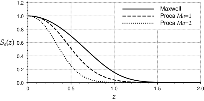
Figure 1: Plot of the scale function $\mathcal{S}_{s}(z)$ for the Gaussian sampling function in the Einstein Universe. Three different cases are of Eq. (144) are displayed: Electromagnetism (solid line) and two cases of the Proca field for different values of the mass times the radius of universe, $Ma=1$ (dashed line) and $Ma=2$ (dotted line). The plots were produced by evaluating the first 3000 terms in the summation of Eq. (144).

is plotted in Figure 1. For very short sampling times the scale function is close to unity and the QWEI bound is the same as that for Minkowski spacetime Pfenning (2002). This makes sense because the spacetime appears to be flat over time scales which are short relative to the radius of the universe, and we should expect to recover the Minkowski space result. As the sampling time becomes progressively longer, the field has more time to “sample” the curvature of the universe, and thus it becomes increasingly difficult to generate negative energy densities. Also, as the mass of the field increases it becomes increasingly difficult to generate negative energy densities. This is seen by the faster decay in the scale functions for larger value of the field mass as seen in previous evaluations of the scale function for scalar fields in other spacetimes Ford and Roman (1997); Pfenning and Ford (1998); Pfenning (1998). As mentioned above, the quantum inequality bound has also been evaluated for electromagnetism with a Lorentzian sampling function Pfenning (2002) and the behaviour is very much the same.

Appendix A Consistency of the Hadamard condition with the constraints

In this appendix we prove the following local-to-global result.

Theorem A.1.

Let $\omega$ be a state on either $\mathfrak{A}_{M}(\mathcal{M},g)$ or $\mathfrak{A}(\mathcal{M},g)$ and suppose that there exists a causal normal neighbourhood $\mathcal{N}$ of a Cauchy surface $\Sigma$ in $\mathcal{M}$, and a Hadamard bisolution $W_{M}$ (respectively, $W$) to $\Box+M^{2}$ (respectively, $\Box$) on $\mathcal{N}\times\mathcal{N}$ such that

$$\omega\left(\mathcal{A}(f_{1})\mathcal{A}(f_{2})\right)=W_{M}\left(f_{1},\left(\hbox{{\rm$\openone$}}-M^{-2}{\bf d}\bm{\delta}\right)f_{2}\right)$$ (145)

for all $f_{i}\in\Omega^{1}_{0}(\mathcal{N})$ (in the Proca case) or

$$\omega\left([\mathcal{A}](f_{1})[\mathcal{A}](f_{2})\right)=W\left(f_{1},f_{2}\right)$$ (146)

for all $f_{i}\in\Omega^{1}_{0}(\mathcal{N})$ with $\bm{\delta}f_{i}=0$ (in the Maxwell case). Then $\omega$ is Hadamard.

Thus the Hadamard conditions introduced in Sect. III.3 respect the Cauchy evolution of the field equations: if they are satisfied near one Cauchy surface, they hold near all others and hence hold globally. As the Hadamard form for Klein–Gordon bisolutions also propagates in this sense, our discussion may be regarded as checking the consistency of the definitions of Sect. III.3 with the Proca and Maxwell constraints. The propagation property is one of the key ingredients used in Sect. IV.5, where we established the existence of Hadamard states on general globally hyperbolic spacetimes obeying our usual topological conditions. Although we will use the fact that $\Sigma$ is compact for both the Maxwell and Proca fields this condition can probably be dropped; however in the Maxwell case it appears to be necessary [in Lemma A.4(b)] to assume that $H_{1}(\Sigma)$ is trivial and that the compact support cohomology group $H^{3}_{c}(\mathcal{M})$ of the spacetime is therefore also trivial.

The proof of Theorem A.1 relies on a number of results concerning the classical Proca, Maxwell and Klein–Gordon fields. One fact which will be used repeatedly is that, for $f\in\Omega_{0}^{1}(\mathcal{M})$, $E_{M}f=0$ if and only if $f\in(\Box+M^{2})\Omega_{0}^{1}(\mathcal{M})$. Indeed, $f=(\Box+M^{2})E_{M}^{+}f$ and since, by hypothesis, $E_{M}^{+}f=E_{M}^{-}f$, the support of $E_{M}^{+}f$ is contained in the compact set $J^{+}({\rm supp}\,f)\cap J^{-}({\rm supp}\,f)$. Our first observation generalises this fact to the Proca field.

Lemma A.2.

Let $M>0$. For $f\in\Omega_{0}^{1}(\mathcal{M})$, $\Delta_{M}f=0$ if and only if $f\in(-\bm{\delta}{\bf d}+M^{2})\Omega_{0}^{1}(\mathcal{M})$.

Proof.

Since $(\openone-M^{-2}{\bf d}\bm{\delta})(-\bm{\delta}{\bf d}+M^{2})=\Box+M^{2}$, sufficiency holds because $E_{M}$ is a Klein–Gordon bisolution. Conversely, $\Delta_{M}f=0$ is equivalent to $E_{M}(\openone-M^{-2}{\bf d}\bm{\delta})f=0$; hence, we have

$$(-{\bf d}\bm{\delta}+M^{2})f=M^{2}(\Box+M^{2})g$$ (147)

for some $g\in\Omega_{0}^{1}(\mathcal{M})$. By applying $\bm{\delta}{\bf d}$ to both sides, we obtain $\bm{\delta}{\bf d}f=(\Box+M^{2})\bm{\delta}{\bf d}g$, which may be subtracted from the previous expression to yield

$$(\Box+M^{2})f=(\Box+M^{2})(-\bm{\delta}{\bf d}+M^{2})g\,.$$ (148)

Since both $f$ and $g$ are compactly supported, we conclude that $f=(-\bm{\delta}{\bf d}+M^{2})g$. $\Box$

Proposition A.3.

(a) Given any $f\in\Omega_{0}^{1}(\mathcal{M})$ there exists $g\in\Omega_{0}^{1}(\mathcal{M})$ such that $\widetilde{f}=f+(-\bm{\delta}{\bf d}+M^{2})g$ is an element of $\Omega_{0}^{1}(\mathcal{N})$.
(b) Given any co-closed $f\in\Omega_{0}^{1}(\mathcal{M})$ there exists $g\in\Omega_{0}^{1}(\mathcal{M})$ such that $\widetilde{f}=f-\bm{\delta}{\bf d}g$ is a co-closed element of $\Omega_{0}^{1}(\mathcal{N})$.

Proof.

(a) Choose smooth functions $\chi^{\pm}$ on $\mathcal{M}$ with $\chi^{+}+\chi^{-}=1$ and $\chi^{+}$ equal to unity to the future of $\mathcal{N}$ and vanishing to the past of $\mathcal{N}$. Then

$$\widetilde{f}=(-\bm{\delta}{\bf d}+M^{2})\chi^{+}\Delta_{M}f$$ (149)

belongs to $\Omega_{0}^{1}(\mathcal{N})$ and satisfies $\Delta_{M}\widetilde{f}=\Delta_{M}f$. Applying Lemma A.2 to $\widetilde{f}-f$, it follows that $\widetilde{f}=f+(-\bm{\delta}{\bf d}+M^{2})g$ as required.
(b) With $\chi^{\pm}$ as above, set $\widetilde{f}=-\bm{\delta}{\bf d}\chi^{+}E_{0}f$. Then $\widetilde{f}$ belongs to $\Omega_{0}^{1}(\mathcal{N})$ and is co-closed; moreover $E_{0}\widetilde{f}$ and $E_{0}f$ are gauge equivalent by the proof of Prop. 4(c) in Dimock (1992). Accordingly, there exists $\eta\in\Omega^{0}(\mathcal{M})$ such that $E_{0}(\widetilde{f}-f)={\bf d}\eta$. Taking co-derivatives, using $\bm{\delta}E_{0}=E_{0}\bm{\delta}$ and co-closure of $\widetilde{f}$ and $f$, we have $\bm{\delta}{\bf d}\eta=0$ and hence $\eta=E_{0}\zeta$ for some $\zeta\in\Omega_{0}^{0}(\mathcal{M})$. Substituting back, we see that $E_{0}(\widetilde{f}-f-{\bf d}\zeta)=0$, so

$$\widetilde{f}-f-{\bf d}\zeta=\Box g$$ (150)

for some $g\in\Omega_{0}^{1}(\mathcal{M})$. Taking co-derivatives again, $\Box(\zeta-\bm{\delta}g)=0$ and hence (because both $\zeta$ and $g$ are compactly supported) $\zeta=\bm{\delta}g$. Substituting back in Eq. (150), we have $\widetilde{f}=f+{\bf d}\bm{\delta}g+\Box g=f-\bm{\delta}{\bf d}g$ as required. $\Box$

Lemma A.4.

(a) If $\mathcal{A}$ is a weak one-form $(\Box+M^{2})$-solution obeying

$$\mathcal{A}((-\bm{\delta}{\bf d}+M^{2})f)=0$$ (151)

for all $f\in\Omega_{0}^{1}(\mathcal{N})$, then Eq. (151) holds for all $f\in\Omega_{0}^{1}(\mathcal{M})$.
(b) If $\mathcal{A}$ is a weak one-form $\Box$-solution vanishing on co-closed $f\in\Omega_{0}^{1}(\mathcal{N})$, then $\mathcal{A}$ vanishes on all co-closed $f\in\Omega_{0}^{1}(\mathcal{M})$.

Proof.

(a) Since, for $f\in\Omega_{0}^{1}(\mathcal{N})$, $\mathcal{A}((\Box+M^{2})f)=0$, we have by Eq. (151) that

$$\mathcal{A}({\bf d}\bm{\delta}f)=0$$ (152)

for all $f\in\Omega_{0}^{1}(\mathcal{N})$. Thus, $\mathcal{A}({\bf d}\cdot)$ is a global weak scalar $(\Box+M^{2})$-solution vanishing on $\bm{\delta}\Omega_{0}^{1}(\mathcal{N})$. Now we may fix $f_{0}\in\Omega_{0}^{0}(\mathcal{N})$ such that any $f\in\Omega_{0}^{0}(\mathcal{N})$ may be written

$$f=f_{0}\int f\,d{\rm vol}_{g}+\bm{\delta}h$$ (153)

for some $h\in\Omega_{0}^{1}(\mathcal{N})$. (Since $\mathcal{N}$ is connected, boundaryless and orientable, this follows by de Rahm’s theorem: see the remarks following Theorem 7.5.19 in Abraham et al. (1988).) Combining Eqs. (152 and (153), we have $\mathcal{A}({\bf d}f)=\mathcal{A}({\bf d}f_{0})\int f\,d{\rm vol}_{g}$ for all $f\in\Omega_{0}^{0}(\mathcal{N})$. Accordingly, $\mathcal{A}({\bf d}\cdot)$ is constant on $\mathcal{N}$ and hence (since it is a $(\Box+M^{2})$-solution) on $\mathcal{M}$. It follows that $\mathcal{A}({\bf d}\bm{\delta}f)=\mathcal{A}({\bf d}f_{0})\int\bm{\delta}f\,d{\rm vol}_{g}=0$ for all $f\in\Omega_{0}^{1}(\mathcal{M})$. Since $\mathcal{A}((\Box+M^{2})f)=0$, we deduce that Eq. (151) holds for all $f\in\Omega_{0}^{1}(\mathcal{M})$ as required.
(b) $\mathcal{A}(\bm{\delta}\cdot)$ is a two-form weak $\Box$-solution vanishing on all $h\in\Omega_{0}^{2}(\mathcal{N})$ and hence on all $h\in\Omega_{0}^{2}(\mathcal{M})$. But since $H^{3}_{c}(\mathcal{M})$ is trivial, any $f\in\Omega_{0}^{1}(\mathcal{M})$ such that $\bm{\delta}f=0$ can be written as $f=\bm{\delta}h$ for some $h\in\Omega_{0}^{2}(\mathcal{M})$ and we conclude that $\mathcal{A}(f)=\mathcal{A}(\bm{\delta}h)=0$. $\Box$

After these preliminaries, we may now prove the main result of this section.
Proof of Theorem A.1. The arguments for the two theories run along parallel lines. First one extends the $W_{M}$ (resp., $W$) to be a global bisolution to the appropriate one-form Klein–Gordon equation. Since the Hadamard form propagates, it suffices to show that Eq. (145) holds for all $f_{i}\in\Omega^{1}_{0}(\mathcal{M})$ (resp., that Eq. (146) holds for all co-closed $f_{i}\in\Omega^{1}_{0}(\mathcal{M})$). In the Proca case, we apply Proposition A.3(a) together with the field equation axiom P3 and Eq. (145) to show that

$$\omega\left(\mathcal{A}(f_{1})\mathcal{A}(f_{2})\right)=\omega\left(\mathcal{A}(\widetilde{f_{1}})\mathcal{A}(\widetilde{f_{2}})\right)=W_{M}(\widetilde{f_{1}},\left(\hbox{{\rm$\openone$}}-M^{-2}{\bf d}\bm{\delta}\right)\widetilde{f_{2}})$$ (154)

for general $f_{i}\in\Omega_{0}^{1}(\mathcal{M})$. In the Maxwell case, we apply Proposition A.3(b), axiom M3 and Eq. (146) to obtain

$$\omega\left([\mathcal{A}](f_{1})[\mathcal{A}](f_{2})\right)=\omega\left([\mathcal{A}](\widetilde{f_{1}})[\mathcal{A}](\widetilde{f_{2}})\right)=W(\widetilde{f_{1}},\widetilde{f_{2}})$$ (155)

for co-closed $f_{i}\in\Omega_{0}^{1}(\mathcal{M})$. The following claim will be proved below.

Proposition A.5.

In the Proca case,

$$W_{M}((-\bm{\delta}{\bf d}+M^{2})f,f^{\prime})=W_{M}(f^{\prime},(-\bm{\delta}{\bf d}+M^{2})f)=0$$ (156)

for all $f,f^{\prime}\in\Omega_{0}^{1}(\mathcal{M})$, while in the Maxwell case, we have

$$W(\bm{\delta}{\bf d}f,f^{\prime})=W(f^{\prime},\bm{\delta}{\bf d}f)=0$$ (157)

for all $f,f^{\prime}\in\Omega_{0}^{1}(\mathcal{M})$ with $f^{\prime}$ co-closed.

In combination with the explicit form of $\widetilde{f}_{i}-f_{i}$ (and, in the Proca case, the fact that $(\openone-M^{-2}{\bf d}\bm{\delta})$ and $-\bm{\delta}{\bf d}+M^{2}$ commute) Prop. A.5 allows us to show that

$$W_{M}(\widetilde{f_{1}},(\openone-M^{-2}{\bf d}\bm{\delta})\widetilde{f_{2}})=W_{M}(f_{1},(\openone-M^{-2}{\bf d}\bm{\delta})f_{2})$$ (158)

in the Proca case, and that $W(\widetilde{f_{1}},\widetilde{f_{2}})=W(f_{1},f_{2})$ holds for the Maxwell field. Taken together with Eqs. (154) and (155) respectively, these relations then establish Eqs. (145) and (146). $\Box$

The claim made above is proved as follows.
Proof of Proposition A.5. Fix an arbitrary $f^{\prime}\in\Omega_{0}^{1}(\mathcal{N})$ (with the additional requirement that $\bm{\delta}f^{\prime}=0$ in the Maxwell case). Then $W_{M}(\cdot,f^{\prime})$ and $W_{M}(f^{\prime},\cdot)$ (or $W(\cdot,f^{\prime})$ and $W(f^{\prime},\cdot)$ in the Maxwell case) obey the hypotheses of Lemma A.4(a) owing to Eq. (145) and axiom P3 (resp., Eq. (146) and axiom M3). Accordingly, Eq. (156) (resp., Eq. (157)) holds for all $f\in\Omega_{0}^{1}(\mathcal{M})$ and the fixed $f^{\prime}\in\Omega_{0}^{1}(\mathcal{N})$. Now fix $f\in\Omega_{0}^{1}(\mathcal{M})$ arbitrarily. In the Proca case, $W_{M}((-\bm{\delta}{\bf d}+M^{2})f,\cdot)$ and $W_{M}(\cdot,(-\bm{\delta}{\bf d}+M^{2})f)$ are weak $(\Box+M^{2})$-solutions vanishing on $\mathcal{N}$ and hence globally, as required. In the Maxwell case, $W(\bm{\delta}{\bf d}f,\cdot)$ and $W(\cdot,\bm{\delta}{\bf d}f)$ are weak $\Box$-solutions vanishing on co-closed elements of $\Omega_{0}^{1}(\mathcal{N})$. Lemma A.4(b) entails that they therefore vanish on all co-closed $f^{\prime}\in\Omega_{0}^{1}(\mathcal{M})$, thereby completing the proof. $\Box$

Appendix B Construction of a Hadamard $(\Box+M^{2})$-bisolution in ultrastatic spacetimes

In this appendix we prove Theorem IV.1 by explicitly constructing a Hadamard $(\Box+M^{2})$-bisolution $W_{M}$ on any ultrastatic spacetime $(\mathcal{M},g)$ obeying the assumptions stated at the beginning of Sect. IV. For $M>0$, the argument proceeds as follows. First, we use functional calculus on the Hilbert space ${\sf H}$ to define $W_{M}$ as a bilinear map from $\Omega_{0}^{1}(\mathcal{M})\times\Omega_{0}^{1}(\mathcal{M})$ to $\mathbb{C}$. We show that $W_{M}$ is in fact a one-form bidistributional weak $(\Box+M^{2})$-bisolution, with antisymmetric part $-iE_{M}$, and determine a crude bound on its wave-front set. Next, we appeal to the existence of a Hadamard $(\Box+M^{2})$-bisolution $\widetilde{W}_{M}$, also with antisymmetric part $-iE_{M}$, established in Lemma 5.4(a) of Sahlmann and Verch (2001). A simple microlocal argument is used to show that $W_{M}-\widetilde{W}_{M}$ is smooth, from which it follows that $W_{M}$ is itself Hadamard. Finally, we show that $W_{M}$ may be expanded in terms of any ${\sf K}$-pseudo-orthonormal complete set of eigenvectors for the operator $K$ as claimed in Theorem IV.1. The argument is only slightly different in the case $M=0$.

It will be convenient to regard each $\mathcal{A}\in\Omega^{1}(\mathcal{M})$ as a smooth one-parameter family $t\mapsto\mathcal{A}(t)$ of elements in ${\sf H}=\Lambda^{0}(\Sigma)\oplus\Lambda^{1}(\Sigma)$, where $\mathcal{A}(t)$ is the restriction of $\mathcal{A}$ to the constant time surface $\{t\}\times\Sigma$. The pairing $\langle\cdot,\cdot\rangle$ of one-forms on $\mathcal{M}$ is related to the inner products of ${\sf H}$ and ${\sf K}$ by

$$\langle\mathcal{A},\mathcal{B}\rangle=\int dt\,\langle\langle\overline{\mathcal{A}(t)}\mid\mathcal{B}(t)\rangle\rangle=\int dt\,\left(\overline{\mathcal{A}(t)},J\mathcal{B}(t)\right)_{\sf H}\,,$$ (159)

where $J=\openone_{\Lambda^{0}(\Sigma)}\oplus-\openone_{\Lambda^{1}(\Sigma)}$. We note that $J$ and $K=(-\Delta^{s}_{\Sigma}+M^{2})\oplus(-\Delta_{\Sigma}+M^{2})$ commute.

With these conventions, the Klein–Gordon equation $(\Box+M^{2})\mathcal{A}=0$ may be written as the Hilbert space ordinary differential equation

$$-\partial_{t}^{2}\mathcal{A}(t)=K\mathcal{A}(t)\,.$$ (160)

Suppose that $M>0$. Because $\Sigma$ is compact, $K$ has discrete spectrum bounded below by $M^{2}>0$. Accordingly, the operator $K^{-1/2}$ is well-defined and bounded, and the advanced-minus-retarded solution operator $E_{M}:\Omega_{0}^{1}(\mathcal{M})\to\Omega^{1}(\mathcal{M})$ may be written

$$(E_{M}\mathcal{J})(t)=\int dt^{\prime}\,K^{-1/2}\sin\left[K^{1/2}(t^{\prime}-t)\right]\mathcal{J}(t^{\prime})\,,$$ (161)

thus obtaining

$$E_{M}(\mathcal{J},\mathcal{J}^{\prime})=\langle\mathcal{J},E_{M}\mathcal{J}^{\prime}\rangle=\int dt\,dt^{\prime}\,\left(\overline{\mathcal{J}(t)},JK^{-1/2}\sin\left[K^{1/2}(t^{\prime}-t)\right]\mathcal{J}^{\prime}(t^{\prime})\right)_{\sf H}\,.$$ (162)

We define our candidate Hadamard $(\Box+M^{2})$-bisolution $W_{M}$ by taking the positive frequency part of $-iE_{M}$, i.e., by replacing the sine function by an exponential. To be precise, for $f,f^{\prime}\in\mathcal{D}(\mathbb{R})$ and $g,g^{\prime}\in\Omega^{0}(\Sigma)\oplus\Omega^{1}(\Sigma)$, we define

$$W_{M}(f\otimes g,f^{\prime}\otimes g^{\prime})=-\frac{1}{2}\left(\widehat{\overline{f}}(K^{1/2})\overline{g},K^{-1/2}\widehat{f^{\prime}}(K^{1/2})Jg^{\prime}\right)_{\sf H}\,,$$ (163)

in which operators such as $\widehat{f^{\prime}}(K^{1/2})$ are defined by functional calculus. Using the Cauchy–Schwarz inequality and elementary operator norm estimates, we find

$$\left|W_{M}(f\otimes g,f^{\prime}\otimes g^{\prime})\right|\leq\frac{1}{2}\|K^{-1/2}\|\,\|g\|\,\|g^{\prime}\|\sup_{\omega\in\sigma(K^{1/2})}|\widehat{f}(-\omega)|\sup_{\omega\in\sigma(K^{1/2})}|\widehat{f^{\prime}}(\omega)|\,,$$ (164)

from which it follows that $W_{M}$ extends to a distribution in $(\Omega_{0}^{1}(\mathcal{M})\times\Omega_{0}^{1}(\mathcal{M}))^{\prime}$. It is straightforward to check that $W_{M}$ is a weak $(\Box+M^{2})$-bisolution, with antisymmetric part $-iE_{M}$.

The wave-front set of $W_{M}$ may be estimated in two ways. First, because it is a $(\Box+M^{2})$-bisolution, we have

$${\rm WF}\,(W_{M})\subseteq\mathcal{N}\times\mathcal{N}$$ (165)

where $\mathcal{N}=\{(x,k)\in T^{*}\mathcal{M}:g^{ab}(x)k_{a}k_{b}=0\}$ is the null bundle of $(\mathcal{M},g)$. Secondly, the explicit bound (164), coupled with the observation that $\sup_{\omega\in\sigma(K^{1/2})}|\widehat{f}(\lambda-\omega)|$ is bounded as $\lambda\to+\infty$, but rapidly decaying for $\lambda\to-\infty$ (and vice versa for $\sup_{\omega\in\sigma(K^{1/2})}|\widehat{f}(\lambda+\omega)|$) entails that

$${\rm WF}\,(W_{M})\subseteq(\mathcal{T}^{+}\cup\mathcal{Z})\times(\mathcal{T}^{-}\cup\mathcal{Z})$$ (166)

where $\mathcal{T}^{\pm}=\{(x,k)\in T^{*}\mathcal{M}:\pm k_{0}>0\}$ and $\mathcal{Z}=\{(x,k)\in T^{*}\mathcal{M}:k=0\}$ is the zero section of $T^{*}\mathcal{M}$. Comparing these two estimates,

$${\rm WF}\,(W_{M})\subseteq(\mathcal{N}^{+}\cup\mathcal{Z})\times(\mathcal{N}^{-}\cup\mathcal{Z})$$ (167)

where $\mathcal{N}^{\pm}=\mathcal{N}\cap\mathcal{T}^{\pm}$ are the future ($+$) and past ($-$) null bundles.

We now appeal to the existence of a Hadamard form $(\Box+M^{2})$-bisolution $\widetilde{W}_{M}$ on $(\mathcal{M},g)$ with antisymmetric part $-iE_{M}$ (Lemma 5.4(a) of Sahlmann and Verch (2001)). Since the wave-front set of $\widetilde{W}_{M}$ also obeys (167), we have

$${\rm WF}\,(W_{M}-\widetilde{W}_{M})\subseteq(\mathcal{N}^{+}\cup\mathcal{Z})\times(\mathcal{N}^{-}\cup\mathcal{Z})\,.$$ (168)

But $W_{M}-\widetilde{W}_{M}$ is symmetric, so we also have

$${\rm WF}\,(W_{M}-\widetilde{W}_{M})\subseteq(\mathcal{N}^{-}\cup\mathcal{Z})\times(\mathcal{N}^{+}\cup\mathcal{Z})\,.$$ (169)

Comparing these two bounds, we see that ${\rm WF}\,(W_{M}-\widetilde{W}_{M})\subseteq\mathcal{Z}\times\mathcal{Z}$ and, since the wave-front set excludes the zero section, we conclude that this wave-front set is in fact empty. Accordingly, $W_{M}=\widetilde{W}_{M}$ (mod $C^{\infty}$) so $W_{M}$ is of Hadamard form.

The analysis of the massless case is complicated by the existence of a zero eigenvalue mode $\varphi_{0}=(1,0)$ for $K$. (Triviality of $H_{1}(\Sigma)$ precludes the existence of any harmonic one-forms on $\Sigma$, so $\varphi_{0}$ is the unique zero mode.) However, the spectrum of $K$ is otherwise bounded away from zero, so $K^{-1/2}$ is well-defined and bounded on $P{\sf H}$, where $P$ is the orthogonal projector onto the orthogonal complement of $\varphi_{0}$. In this case, we define

$$W(f\otimes g,f^{\prime}\otimes g^{\prime})=-\frac{1}{2}\left(\widehat{\overline{f}}(K^{1/2})P\overline{g},K^{-1/2}\widehat{f^{\prime}}(K^{1/2})PJg^{\prime}\right)_{\sf H}\,.$$ (170)

It is easy to check that $W$ is a bidistributional $\Box$-bisolution, whose antisymmetric part is

$$W(\mathcal{J},\mathcal{J}^{\prime})-W(\mathcal{J}^{\prime},\mathcal{J})=-iE_{0}(\mathcal{J},\mathcal{J}^{\prime})+i\int dt\,dt^{\prime}\,(t^{\prime}-t)\,(\overline{\mathcal{J}(t)},\,\varphi_{0})_{\sf H}\,(\varphi_{0},J\mathcal{J}^{\prime}(t^{\prime}))_{\sf H}$$ (171)

and is therefore equal (mod $C^{\infty}$) to $-iE_{0}$. Appealing as before to the existence of a Hadamard $\Box$-bisolution $\widetilde{W}$ with antisymmetric part $-iE_{0}$, the argument used above shows that $W=\widetilde{W}$ (mod $C^{\infty}$) because $W-\widetilde{W}$ is symmetric (mod $C^{\infty}$). It remains to show that the last term in Eq. (171) vanishes if $\mathcal{J}$ and $\mathcal{J}^{\prime}$ are both co-closed, as required for consistency with the commutator axiom M4. Using Eq. (159) and the fact that $J\varphi_{0}=\varphi_{0}$, one may show that the term in question is proportional to $\langle\overline{\mathcal{J}},{\bf d}t\rangle\,\langle t{\bf d}t,\mathcal{J}^{\prime}\rangle-\langle\overline{\mathcal{J}},t{\bf d}t\rangle\,\langle{\bf d}t,\mathcal{J}^{\prime}\rangle$, which vanishes because $\langle\overline{\mathcal{J}},{\bf d}t\rangle=\langle\overline{\bm{\delta}\mathcal{J}},t\rangle=0$ and similarly $\langle{\bf d}t,\mathcal{J}^{\prime}\rangle=0$.

Finally, let $\xi_{j}$ be a complete set of ${\sf K}$-pseudo-orthonormal $K$-eigenfunctions, with corresponding eigenvalues $\omega_{\lambda}^{2}$ ($\omega_{\lambda}\geq 0$). Using the completeness relation Eq. (43), we see that

$$\widehat{f^{\prime}}(K^{1/2})^{*}K^{-1/2}\widehat{\overline{f}}(K^{1/2})P\overline{g}=\sum_{j:\omega_{j}\not=0}\xi_{j}\omega_{j}^{-1}\overline{\widehat{f^{\prime}}(\omega_{j})}\widehat{\overline{f}}(\omega_{j})\langle\langle\xi_{j}\mid\xi_{j}\rangle\rangle\,\langle\langle\xi_{j}\mid\overline{g}\rangle\rangle$$ (172)

and hence

$$W(\mathcal{J},\mathcal{J}^{\prime}) = -\sum_{j:\omega_{j}\not=0}\frac{1}{2\omega_{j}}\langle\langle\xi_{j}\mid\xi_{j}\rangle\rangle\,\langle\langle\widehat{\overline{f}}(\omega_{j})\overline{g}\mid\xi_{j}\rangle\rangle\langle\langle\xi_{j}\mid\widehat{f^{\prime}}(\omega_{j})g^{\prime}\rangle\rangle$$ (173)

$$= -\sum_{j:\omega_{j}\not=0}\frac{1}{2\omega_{j}}\langle\langle\xi_{j}\mid\xi_{j}\rangle\rangle\,\langle\mathcal{A}_{j},\mathcal{J}\rangle\,\langle\overline{\mathcal{A}_{j}},\mathcal{J}^{\prime}\rangle\,,$$

where we have defined the modes $\mathcal{A}_{j}$ by $\mathcal{A}_{j}(t)=e^{-i\omega_{j}t}\xi_{\lambda}$ and used

$$\langle\langle\xi_{j}\mid\widehat{f^{\prime}}(\omega_{j})g^{\prime}\rangle\rangle=\int dt\,e^{i\omega_{j}t}\langle\langle\xi_{j}\mid f^{\prime}(t)g^{\prime}\rangle\rangle=\int dt\,\langle\langle\mathcal{A}_{j}(t)\mid\mathcal{J}^{\prime}(t)\rangle\rangle=\langle\overline{\mathcal{A}_{j}},\mathcal{J}^{\prime}\rangle$$ (174)

and $\langle\langle\widehat{\overline{f}}(\omega_{j})\overline{g}\mid\xi_{j}\rangle\rangle=\langle\mathcal{J},\mathcal{A}_{j}\rangle=\langle\mathcal{A}_{j},\mathcal{J}\rangle$.

In the case $M>0$, exactly analogous arguments show that the $W_{M}(\mathcal{J},\mathcal{J}^{\prime})$ may also be written in the form of the right-hand side of Eq. (173) [the restriction to $\omega_{j}>0$ is inessential as all modes obey this condition]. This completes the proof of Theorem IV.1.

References

• Penrose (1965) R. Penrose, Phys. Rev. Lett. 14, 57 (1965).
• Hawking (1965) S. W. Hawking, Phys. Rev. Lett. 15, 689 (1965).
• Epstein et al. (1965) H. Epstein, V. Glaser, and A. Jaffe, Il Nuovo Cim. 36, 1016 (1965).
• Morris and Thorne (1988) M. S. Morris and K. S. Thorne, Am. J. Phys. 56, 395 (1988).
• Morris et al. (1988) M. S. Morris, K. S. Thorne, and U. Yurtsever, Phys. Rev. Lett. 61, 1446 (1988).
• Hiscock (1981) W. A. Hiscock, Ann. Phys. 131, 245 (1981).
• Ford and Roman (1992) L. H. Ford and T. A. Roman, Phys. Rev. D 46, 1328 (1992).
• Alcubierre (1994) M. Alcubierre, Class. Quantum Grav. 11, L73 (1994).
• Krasnikov (1998) S. V. Krasnikov, Phys. Rev. D 57, 4760 (1998), gr-qc/9511068.
• Everett (1996) A. E. Everett, Phys. Rev. D 53, 7365 (1996).
• Parker and Fulling (1973) L. Parker and S. A. Fulling, Phys. Rev. D 7, 2357 (1973).
• Ford (1978) L. H. Ford, Proc. Roy. Soc. Lond. A 364, 227 (1978).
• Ford (1991) L. H. Ford, Phys. Rev. D 43, 3972 (1991).
• Ford and Roman (1995) L. H. Ford and T. A. Roman, Phys. Rev. D 51, 4277 (1995), gr-qc/9410043.
• Ford and Roman (1997) L. H. Ford and T. A. Roman, Phys. Rev. D 55, 2082 (1997), gr-qc/9607003.
• Pfenning and Ford (1997) M. J. Pfenning and L. H. Ford, Phys. Rev. D 55, 4813 (1997), gr-qc/9608005.
• Pfenning and Ford (1998) M. J. Pfenning and L. H. Ford, Phys. Rev. D 57, 3489 (1998), gr-qc/9710055.
• Pfenning (1998) M. J. Pfenning, Ph.D. thesis, Tufts University, Medford, Massachusetts (1998), gr-qc/9805037.
• Flanagan (1997) É. É. Flanagan, Phys. Rev. D 56, 4922 (1997), gr-qc/9706006.
• Flanagan (2002) É. É. Flanagan, Phys. Rev. D 66, 104007 (2002), gr-qc/0208066.
• Vollick (2000) D. N. Vollick, Phys. Rev. D 61, 084022 (2000).
• Fewster and Eveson (1998) C. J. Fewster and S. P. Eveson, Phys. Rev. D 58, 084010 (1998), gr-qc/9805024.
• Fewster and Teo (1999) C. J. Fewster and E. Teo, Phys. Rev. D 59, 104016 (1999).
• Fewster (2000) C. J. Fewster, Class. Quantum Grav. 17, 1897 (2000).
• Fewster and Verch (2002) C. J. Fewster and R. Verch, Commun. Math. Phys. 225, 331 (2002).
• (26) A. D. Helfer, hep-th/9908012.
• Pfenning (2002) M. J. Pfenning, Phys. Rev. D 65, 024009 (2002).
• Marecki (2002) P. Marecki, Phys. Rev. A 66, 053801 (2002), quant-ph/0203027.
• Radzikowski (1996) M. J. Radzikowski, Commun. Math. Phys. 179, 529 (1996).
• Kratzert (2000) K. Kratzert, Annalen Phys. 9, 475 (2000).
• Hollands (2001) S. Hollands, Commun. Math. Phys. 216, 635 (2001).
• Sahlmann and Verch (2001) H. Sahlmann and R. Verch, Rev. Math. Phys. 13, 1203 (2001), math-ph/0008029.
• Brown and Ottewill (1986) M. R. Brown and A. C. Ottewill, Phys. Rev. D 34, 1776 (1986).
• Allen and Ottewill (1992) B. Allen and A. C. Ottewill, Phys. Rev. D 46, 861 (1992).
• (35) W. Junker and F. Lledó, in preparation.
• Dimock (1992) J. Dimock, Rev. Math. Phys. 4, 223 (1992).
• Furlani (1999) E. P. Furlani, J. Math. Phys. 40, 2611 (1999).
• Fulling et al. (1981) S. A. Fulling, F. J. Narcowich, and R. M. Wald, Ann. Phys. 136, 243 (1981).
• Abraham et al. (1988) R. Abraham, J. E. Marsden, and T. Ratiu, Manifolds, Tensor Analysis, and Applications (Springer-Verlag, New York, 1988), 2nd ed.
• Hörmander (1983) L. Hörmander, The Analysis of Linear Partial Differential Operators, vol. I (Springer-Verlag, Berlin, 1983), 2nd ed.
• Dieckmann (1988) J. Dieckmann, J. Math. Phys. 29, 578 (1988).
• Choquet-Bruhat (1968) Y. Choquet-Bruhat, Batelle Rencontres (Benjamin, New York, 1968), chap. IV, pp. 84–106.
• Strohmaier (2000) A. Strohmaier, Commun. Math. Phys. 215, 105 (2000).
• Strocchi (1967) F. Strocchi, Phys. Rev. 165, 1429 (1967).
• Strocchi (1970) F. Strocchi, Phys. Rev. D 2, 2334 (1970).
• Baez et al. (1992) J. Baez, I. Segal, and Z. Zhou, Introduction to Algebraic and Constructive Quantum Field Theory (Princeton University Press, Princeton, 1992).
• Kay and Wald (1991) B. S. Kay and R. M. Wald, Phys. Rep. 207, 49 (1991).
• Lledó (2000) F. Lledó, talk at the meeting on Microlocal Analysis and Quantum Field Theory, Mathematisches Forschungsinstitut Oberwolfach (2000).
• Cycon et al. (1987) H. L. Cycon, R. G. Froese, W. Kirsch, and B. Simon, Schrödinger Operators (Springer-Verlag, Berlin, 1987).
• Gupta (1950) S. N. Gupta, Proc. Phys. Soc. London A63, 681 (1950).
• Gupta (1977) S. N. Gupta, Quantum Electrodynamics (Gordon and Breach Science Publishers, Inc., New York, 1977).
• Hörmander (1971) L. Hörmander, Acta Math. 127, 79 (1971).
• Grundling and Lledó (2000) H. Grundling and F. Lledó, Rev. Math. Phys. 12, 1159 (2000).
• Itzykson and Zuber (1980) C. Itzykson and J.-B. Zuber, Quantum Field Theory (McGraw-Hill, Inc., New York, 1980).
• (55) C. J. Fewster and R. Verch, to appear in Commun. Math. Phys., math-ph/0203010.
• Lifshitz (1946) E. M. Lifshitz, J. Phys. (Moscow) 10, 116 (1946).
• Parker (1972) L. Parker, Phys. Rev. D 5, 2905 (1972).
• Mashhoon (1973) B. Mashhoon, Phys. Rev. D 8, 4297 (1973).
• Parker and Fulling (1974) L. Parker and S. A. Fulling, Phys. Rev. D 9, 341 (1974).
• Ford (1976) L. H. Ford, Phys. Rev. D 14, 3304 (1976).
• Jackson (1962) J. D. Jackson, Classical Electrodynamics (John Wiley & Sons, New York, 1962), 2nd ed., see Section 7.5.
• Gradshteyn and Ryzhik (1994) I. S. Gradshteyn and I. M. Ryzhik, Table of Integrals, Series, and Products (Academic Press, San Diego, 1994), 5th ed.
• Bott and Tu (1982) R. Bott and L. W. Tu, Differential forms in algebraic topology (Springer, New York, 1982).
• Warner (1971) F. W. Warner, Foundations of Differentiable Manifolds and Lie Groups (Scott, Foresman and Company, Glenview, 1971).
• Adams (1975) R. Adams, Sobolev Spaces (Academic Press, New York, 1975).
Refer to caption