Tracking Black Holes in Numerical Relativity

Abstract

This work addresses and solves the problem of generically tracking black hole event horizons in computational simulation of black hole interactions. Solutions of the hyperbolic eikonal equation, solved on a curved spacetime manifold containing black hole sources, are employed in development of a robust tracking method capable of continuously monitoring arbitrary changes of topology in the event horizon, as well as arbitrary numbers of gravitational sources. The method makes use of continuous families of level set viscosity solutions of the eikonal equation with identification of the black hole event horizon obtained by the signature feature of discontinuity formation in the eikonal’s solution. The method is employed in the analysis of the event horizon for the asymmetric merger in a binary black hole system. In this first such three dimensional analysis, we establish both qualitative and quantitative physics for the asymmetric collision; including: 1. Bounds on the topology of the throat connecting the holes following merger, 2. Time of merger, and 3. Continuous accounting for the surface of section areas of the black hole sources.

I Introduction

The idea of a totally collapsed gravitational source, from which nothing — not even light — can escape, is an old one, dating back at least to the work of Laplace (and others) in the eighteenth century [1]. Since those original considerations, research has uncovered a wealth of understanding regarding the physics of black holes. In general, the work has followed two major routes, with an ever - narrowing gap between the approaches. Along one direction, black holes are studied as mathematical solutions in a given theory of gravity including Newtonian theory, post-Newtonian metric theories of gravity, Einsteinian gravity, as well as semi-classical and (more recently) various attempts at full quantum theories of gravity. The second direction considers black holes in the astrophysical and astronomical contexts. Both fields of research have seen increasing activity over the years and have made startling discoveries concerning the physics of black holes; including the gravitational collapse theory of Oppenheimer and Snyder [2], proofs of uniqueness and stability of black holes in Einstein’s general relativity [3], thermodynamic properties of black holes including the three laws of black hole mechanics [4] and mechanisms for black hole radiation and evaporation [5], discovery of critical phenomena in black hole formation [6], experimental identification of both astrophysical black hole sources themselves [7] and their event horizons [8], experimental signatures for super - massive black holes in galactic centers [9], and experimental bounds on the distribution and spectrum of black hole sources and collisions [10].

Numerical relativity, which addresses computational solution of Einstein’s equation [11], is an active participant in both the mathematical and the astrophysical programmes of research. With the advent of the Laser Interferometric Gravitational Observatory and other similar efforts, considerable attention has focused on the generic binary black hole coalescence (BBHC) problem, expected as the strongest sources for gravitational waves [12]. As discussed in [11], this is a very difficult and interesting problem that can only successfully be addressed in the computational domain. Consequently, the binary black hole coalescence problem has become an active subject of numerical relativity. One particular problem in the computational domain is the computational definition, detection and tracking of the black hole event horizon itself [13], [14], [15], [16], [17], [18].

The present work completely solves the problem of numerically tracking black hole event horizons. The solution is complete in the sense that a single method is presented such that any one implementation of the method can generically detect arbitrary numbers of black hole event horizons undergoing arbitrarily strong gravitational interactions. For example, using a single computational code of our method we analyse both single black holes and black holes undergoing merger; and no special modifications of our code are required to handle these distinct dynamics.

The present article, describing our generic method for tracking black hole event horizons, is divided as follows. In section II the eikonal equation, the foundation of our method, is described in sufficient detail to be employed in an event horizon tracker. In particular, we focus on the signature behavior of a black hole event horizon in solutions of the eikonal equation. As usual in numerical work, there are a variety of possible implementations of the approach. In section III, several closely related systems of equations are presented and one particular system is singled out for consideration. The system chosen makes use of an explicit second order diffusion, or viscosity, term and we show in section III the relationship between solutions of the diffusive equations of motion and the continuum eikonal equation of interest. Section IV details extraction of the two dimensional sections of the event horizon for each time level of a numerical evolution. Such extraction is crucial for carrying out area, mass, and spin calculations. Section IV also shows the accuracy of our implementation by considering a parameter space survey of single Kerr black holes. Sections V - X describe in detail the first three dimensional application of our (or any) method to the numerical analysis of the asymmetric binary black hole coalescence problem. In particular we search for evidence of any nontrivial topology of the horizon immediately following merger. In distinction to the prediction of [23] we find a topologically spherical horizon to within the accuracy of our three dimensional mesh. Further, area analysis of the candidate numerical event horizon is carried out in conjunction with analysis of the black hole apparent horizons, which reveals both a time of merger much earlier then estimated using apparent horizons and mass energy estimates much larger those found using apparent horizon tracking methods. Our conclusions are presented in section XI.

II The Eikonal

To begin, since the Lagrangian $L=g_{ab}\dot{x}^{a}\dot{x}^{b}$ of null geodesic motion has only kinetic terms it is equal to the associated Hamiltonian. Legendre transformation

$$H\left(\tau,x^{a},p_{b}\right)=\frac{d{x}^{c}}{d\tau}p_{c}-L\left(\tau,x^{d},\frac{d{x}^{e}}{d\tau}\right)$$ (1)

where

$$p_{a}\equiv\frac{\partial L}{\partial\left(\frac{d{x}^{a}}{d\tau}\right)},$$ (2)

sets $L=H$. The corresponding Hamiltonian equations are

$$\frac{d{x}^{a}}{d\tau}=\frac{\partial H}{\partial p_{a}}=2g^{ab}p_{b}$$ (3)

$$\frac{d{p}_{b}}{d\tau}=-\partial_{b}H=-p_{c}p_{d}\partial_{b}g^{cd}.$$ (4)

It is generic that the spacetime metric is independent of the affine parameter $\tau$. There is thus a first integral associated to geodesic motion. Making use of this property permits elimination of the affine parameter in favor of coordinate time $t$. To see this, it is convenient to adopt the ADM variables

$$g^{tt}=\frac{1}{\alpha^{2}},g^{ti}=\frac{\beta^{i}}{\alpha^{2}},g^{ij}=\gamma^{ij}-\frac{\beta^{i}\beta^{j}}{\alpha^{2}}.$$ (5)

Here $\gamma^{ij}$ is the inverse spatial metric. Substituting the ADM variables directly into the Hamiltonian gives

$$H=p_{a}g^{ab}p_{b}=-\frac{1}{\alpha^{2}}p_{t}^{2}+\frac{2}{\alpha^{2}}\beta^{i}p_{i}+p_{i}\left(\gamma^{ij}-\frac{1}{\alpha^{2}}\beta^{i}\beta^{j}\right)p_{j}.$$ (6)

Since the Hamiltonian is not explicitly $\tau$ dependent there is a constant of the motion

$$-\frac{1}{\alpha^{2}}p_{t}^{2}+\frac{2}{\alpha^{2}}\beta^{i}p_{i}+p_{i}\left(\gamma^{ij}-\frac{1}{\alpha^{2}}\beta^{i}\beta_{j}\right)p_{j}=\omega^{2}.$$ (7)

For $\omega^{2}<0$, $\omega^{2}=0$, or $\omega^{2}>0$ the motion is said to be timelike, null, or spacelike. Without loss of generality, assuming null geodesic motion, solution of (7) by ordinary algebra yields:

$$p_{t}=\beta^{i}p_{i}\pm\alpha\sqrt{p_{i}\gamma^{ij}p_{j}}.$$ (8)

With this result, the Hamiltonian can be explicitly factored:

$$H=H_{+}H_{-}=0$$ (9)

where

$$H_{\pm}=p_{t}-\beta^{i}p_{i}\pm\alpha\sqrt{p_{i}\gamma^{ij}p_{j}}=0.$$ (10)

In the case of either root Hamilton’s canonical equations become

$$\frac{dt}{d\tau}=H_{\mp}\frac{\partial H_{\pm}}{\partial p_{t}}=H_{\mp}$$ (11)

$$\frac{dx^{i}}{d\tau}=H_{\mp}\frac{\partial H_{\pm}}{\partial p_{i}}=H_{\mp}\left(-\beta^{i}\pm\alpha\frac{\gamma^{ij}p_{j}}{\sqrt{p_{k}\gamma^{kl}p_{l}}}\right)$$ (12)

$$\frac{dp_{t}}{d\tau}=-H_{\mp}\frac{\partial H_{\pm}}{\partial t}$$ (13)

$$\frac{dp_{i}}{d\tau}=-H_{\mp}\frac{\partial H_{\pm}}{\partial x^{i}}.$$ (14)

According to equation (11), $\tau$ can be eliminated in favor of $t$. The system of equations becomes simply the equations (12) and (14) with $t$ written in place of $\tau$ and the factor $H_{\mp}$ cancelled everywhere on the right hand side. Explicitly,

$$\frac{dx^{i}}{dt}=-\beta^{i}\pm\alpha\frac{\gamma^{ij}p_{j}}{\sqrt{p_{k}\gamma^{kl}p_{l}}}$$ (15)

and

$$\frac{dp_{i}}{dt}=-\partial_{i}\left(-\beta^{j}p_{j}\pm\alpha\sqrt{p_{j}\gamma^{jk}p_{j}}\right).$$ (16)

The eikonal, corresponding to the Hamiltonian of equation (6),

$$\partial_{a}Sg^{ab}\partial_{b}S=0$$ (17)

can be factored similarly. To do so it is a simple matter of making the replacements $p_{t}\rightarrow\partial_{t}S$, $p_{i}\rightarrow\partial_{i}S$ in (8) to find the following symmetric hyberbolic partial differential equation

$$\partial_{t}S=\beta^{i}\partial_{i}S\pm\alpha\sqrt{\partial_{i}S\gamma^{ij}\partial_{j}S}\equiv\bar{H}.$$ (18)

Note that a bar is introduced here to distinguish the Hamiltonian used here from the Hamiltonian used in (6). This equation is also used in the method of [13], although in that work the equation is further reduced to consider the case of a single null surface.

The right hand side of this result is homogeneous of degree one in $\partial_{i}S$. The characteristic curves along which the level sets $\Gamma$ of $S$ are propagated, are then

$$\dot{x}^{i}=-\beta^{i}\pm\alpha\frac{\partial^{i}S}{\sqrt{\partial_{i}S\gamma^{ij}\partial_{j}S}}\equiv\frac{\partial\bar{H}}{\partial\left(\partial_{i}S\right)}$$ (19)

$$\partial_{i}\dot{S}=\partial_{i}\bar{H}\left(t,x^{j},\partial_{j}S\right),$$ (20)

which are the null geodesics of equations (15) and (16). Immediately, the integral curves of the gradients of $S$ and $\Gamma$ are also the null geodesics:

$$\frac{dx^{i}\left(\lambda\right)}{d\lambda}=g^{ia}p_{a}=g^{ia}\partial_{a}S=\partial^{i}S\left(\lambda,x^{j}\left(\lambda\right)\right).$$ (21)

Hereafter, the bar on $\bar{H}$ is dropped with the understanding that the Hamiltonian considered is that of equation (18). This result establishes that the eikonal is technically a Riemann invariant of the null geodesics, a fact that proves useful in establishing the signature of a black hole event horizon in solutions of the eikonal equation. More specifically, since the eikonal is the canonical generator of null geodesics, it can be employed in analysis of black hole event horizons, which are by definition generated by null geodesics having no future end points. To proceed in this manner the equation (18) is employed in an initial value problem and then surveyed for signature features of black hole event horizons.

A black hole event horizon is generated by a congruence of outgoing — but future asymptotically nonexpanding — null geodesics. The scope of the surveys of the eikonal equation that are required to identify a black hole event horizon is then restricted to the space of all outgoing null surfaces. These surveys are greatly reduced by the fact that solutions of the eikonal are categorized by topologically equivalent solutions. To see this, note that

$$\partial_{i}\psi\left(S\right)=\frac{\partial\psi}{\partial S}\partial_{i}S=\lambda\left(S\right)\partial_{i}S,$$ (22)

and

$$\partial_{t}\psi\left(S\right)=\frac{\partial\psi}{\partial S}\partial_{t}S=\lambda\left(S\right)\partial_{t}S.$$ (23)

By homogeneity of the right hand side of (18), if $S$ is a solution then $\psi\left(S\right)$ is also solution. Thus smoothly related initial data $S_{0}\rightarrow S_{0}^{\prime}=\psi\left(S_{0}\right)$ have smoothly related solutions. This feature alleviates the need for surveying over smoothly related initial data.

A further reduction of the scope of solution surveys is provided by the equivalence of ingoing and outgoing solutions under time reversal. Propagation of data for $S$ describing an ingoing or outgoing null surface is accomplished by specification of: 1. A definition of the direction of time, 2. A choice of $\alpha$ and $\beta^{i}$, and 3. A choice of the root. With these choices specified, data is then uniquely partitioned into an ingoing type and an outgoing type with the distinction being the gradient of $S$.

With the dynamics of any outgoing null surface (including the event horizon) specified by (18), and the scope of solution surveys categorized into topological classes, the task remains of identifying the event horizon within this restricted space of outgoing null surfaces. To do so, the results and approach of [13] are adopted here and modified to include the eikonal equation as discussed above. The result of this approach is a signature feature of black hole event horizons in the eikonal equation.

An event horizon of a black hole is by definition a critical outgoing surface when tracked into the future. Let $\mathcal{P}$ be a point interior to the horizon and $\mathcal{Q}$ be a point exterior to the horizon such that $\mathcal{P}$ and $\mathcal{Q}$ lie on characteristic curves of the eikonal $\gamma_{{\mathcal{P}}}$ and $\gamma_{{\mathcal{Q}}}$. At arbitrarily early times let $\gamma_{{\mathcal{P}}}$ and $\gamma_{{\mathcal{Q}}}$ pass arbitrarily closely to a point $\mathcal{H}$ that lies on the horizon $\Gamma$. Since $S$ is a Riemann invariant, at arbitrarily early times the jump of the eikonal at $\mathcal{H}$ becomes $\left[\left[S\left(\mathcal{H}\right)\right]\right]\equiv S_{-}\left(\mathcal{H}\right)-S_{+}\left(\mathcal{H}\right)\approx S\left(\mathcal{P}\right)-S\left(\mathcal{Q}\right)\neq 0$. In the computational domain, where the resolution is finite, this discontinuity will appear generically in finite time. As such, an approximation of the event horizon will appear numerically as the formation of a jump discontinuity in the eikonal for outgoing data that is propagated into the past. This is the numerical signature of black hole event horizons in the eikonal’s solutions.

III Numerical Methods

Analysis of the continuum properties of the eikonal equation as a Hamilton Jacobi equation identifies three closely related approaches to tracking black hole event horizons:

• System I: The null geodesic equations

  $$S\left(x^{j},t\right)=S_{0}\left(x^{k}\right)-\int dtH\left(t,x^{i},p_{i}\right)$$ (24)

  where the integral is evaluated along the solutions of

  $$\dot{x}^{i} = \beta^{i}\pm\alpha\frac{p^{i}}{\sqrt{p_{i}\gamma^{ij}p_{j}}},$$ (25)

  $$\dot{p}_{i} = -\partial_{i}H.$$ (26)

• System II: The eikonal

  $$\partial_{t}S=-H\left(t,x^{j},\partial_{j}S\right)$$ (28)

• System III: The flux conservative form

  $$S\left(x^{i},t\right)=\oint dx^{i}p_{i}\left(x^{j},t\right)$$ (29)

  $$\partial_{t}p_{i}\left(x^{i},t\right)+\partial_{i}H\left(t,x^{j},p_{j}\right)=0.$$ (30)

In each of the above three systems of equations the Hamiltonian is given by (18).

In each of the above cases, the structure of the dynamical equations provide certain advantages. For example, in each case the symplectic structure can be employed to identify numerical loss of accuracy in a similar manner to some modern numerical schemes used in Hamiltonian dynamics. Further, as a flux conservative system, high resolution methods from computational fluid dynamics can be applied directly to the third system. In following sections of this article, the second system is considered since this system of equations yields an expedient implementation that is sufficiently accurate for our purposes.

Singular behavior on the eikonal is not specific to only the event horizon and instead, as described in detail by Arnold and Newman [19], [20], [21], the eikonal is known to generically break down on caustic and other sets. Special numerical methods are then required to handle the generic singular behavior of the eikonal; we make use of an explicit viscosity term. In the continuum, addition of our form of numerical viscosity at the level of the finite difference approximation corresponds to replacing the evolution of

$$\partial_{t}S=-H\left(t,x^{i},\partial_{j}S\right)$$ (31)

with evolution of the equation

$$\partial_{t}\psi=\epsilon^{2}\nabla^{2}\psi-H\left(t,x^{i},\partial_{j}\psi\right)$$ (32)

where $\epsilon$ is a small quantity which we call the viscosity and $\nabla^{2}$ denotes any second order, linear derivative operator. There is a well defined sense in which the solutions $S$ relate to the solutions $\psi$; it is simply given (when the solutions $S$ exist) by the WKB transformation

$$\psi\left(x^{i},t\right)=\sum_{n}a_{n}\left(x^{i},t\right)\epsilon^{n}\exp\left(S/\epsilon\right)\equiv A\exp(S/\epsilon).$$ (33)

To see the explicit relationship between the solutions $\psi$ and the solutions $S$ note that

$$\partial_{t}\psi=\frac{\psi}{\epsilon}\left(\partial_{t}S+\epsilon\partial_{t}\log A\right),$$ (34)

$$\partial_{i}\psi=\frac{\psi}{\epsilon}\left(\partial_{i}S+\epsilon\partial_{i}\log A\right),$$ (35)

$$\nabla^{2}\psi=\frac{\psi}{\epsilon^{2}}\left(\nabla S+\epsilon\nabla\log A\right)^{2}+\frac{\psi}{\epsilon}\left(\nabla^{2}S+\epsilon\nabla^{2}\log A\right).$$ (36)

Assuming that the Hamiltonian is homogeneous of degree one in momentum, and making use of perturbation theory:

$$H\left(x^{i},\nabla_{j}\psi\right)=\frac{\psi}{\epsilon}\left(H\left(x^{i},\nabla_{j}S\right)+\epsilon H_{1}\left(t,x^{i},\partial_{j}\log A\right)\right).$$ (37)

Substituting these results into (32) and cancelling an overall factor of $\psi/\epsilon$ gives at lowest, and first order:

$$\partial_{t}S=-H\left(t,x^{i},\partial_{j}S\right).$$ (38)

$$\epsilon\partial_{t}\log A = -\epsilon H_{1}\left(t,x^{i},\partial_{j}\log A\right)$$ (39)

$$+ \epsilon\left(\nabla S+\epsilon\nabla\log A\right)^{2}+\ldots$$ (40)

Here $H_{1}$ is the first order linear Hamiltonian obtained from perturbation theory. At zeroth order, $S$ then satisfies the eikonal equation, while the first order correction is the linear result of first order perturbation theory and expresses the evolution of $A$. Higher order results can be found similarly. Again, these results hold only where solutions of $S$ exist; that is, away from discontinuities or other solution singularities in $S$ and its derivatives.

The above analysis is a slight modification of usual WKB expansion and expresses the solutions $\psi$ in terms of the solutions $S$. Such solutions can be inverted using the conventional method of series inversion. To invert the WKB expression, and express the solutions of the eikonal in terms of the solution of the parabolic equation, assume first that the solution of the parabolic equation (32) is given as $\psi$ (numerically or otherwise). Writing

$$S=\log\left(\frac{\psi}{\bar{A}}\right),$$ (42)

the procedure is then analogous to that of the WKB expansion: $\bar{A}$ is constructed as an asymptotic power series with coefficients depending on $\psi$ alone. The result of such an analysis is simply:

$$S\left(x,t\right)=\log\psi\left(x,t\right)+\bar{\epsilon}\int dt^{\prime}\frac{\nabla^{2}\psi\left(\bar{x},t\right)}{\psi}$$ (43)

where the integral is evaluated along

$$\frac{d\bar{x}^{i}}{dt}=\frac{\partial H\left(t,\bar{x}^{j},\partial_{\bar{x}^{k}}\log\psi\right)}{\partial p_{i}}$$ (44)

and $\psi$ is provided independently by (numerical) solution of

$$\partial_{t}\psi=\bar{\epsilon}\nabla^{2}\psi-H\left(t,x^{i},\partial_{j}\psi\right).$$ (45)

One advantage of an explicit second order viscosity term is a simple procedure for reducing the error of viscosity solutions by one order of the viscosity $\epsilon$. The limit $\epsilon\rightarrow 0$ corresponds to a continuous family of zeroth order solutions $\phi_{\epsilon}$; where

$$\phi_{\epsilon}=S+\eta_{\epsilon}$$ (46)

and $\eta_{\epsilon}={\mathcal{O}}\left(\epsilon\right)$. Note that each solution $\phi_{\epsilon}$ is obtained from an analysis similar to that following equation (42), although obtained by neglecting the logarithm.

Given two viscosity solutions $\phi_{\epsilon}$ and $\phi_{2\epsilon}$ it is then possible to construct a third improved viscosity solution $\phi_{I}$ that is accurate to ${\mathcal{O}}\left(\epsilon^{2}\right)$. To see this, consider the combination

$$\phi_{I}\equiv\phi_{\epsilon}+\left(\phi_{\epsilon}-\phi_{2\epsilon}\right).$$ (47)

$\phi_{I}$ is accurate to ${\mathcal{O}}\left(\epsilon^{2}\right)$ since

$$\phi_{\epsilon}-\phi_{2\epsilon}=\eta_{\epsilon}-\eta_{2\epsilon}\approx\eta_{\epsilon}-2\eta_{\epsilon}=-\eta_{\epsilon}.$$ (48)

To make use of these improved viscosity solutions let $h$ denote the resolution of the numerical mesh. Any second order finite difference approximation will have then

$$\phi=\hat{\phi}+{\mathcal{O}}\left(h^{2}\right),$$ (49)

where $\phi$ is the continuum solution and $\hat{\phi}$ denotes its finite difference approximation.[We will use a hat throughout the paper to denote the discrete approximation to a continuum object.] Similarly,

$$S=\hat{S}+{\mathcal{O}}\left(h^{2}\right).$$ (50)

Using

$$S=\phi+{\mathcal{O}}\left(\epsilon\right)=\phi_{I}+{\mathcal{O}}\left(\epsilon^{2}\right)$$ (51)

gives

$$\hat{S}=\hat{\phi}+{\mathcal{O}}\left(h^{2}\right)+{\mathcal{O}}\left(\epsilon\right)=\hat{\phi_{I}}+{\mathcal{O}}\left(h^{2}\right)+{\mathcal{O}}\left(\epsilon^{2}\right).$$ (52)

IV Level Set Extraction

Of crucial interest in the binary black hole coalescence problem are the areas of sections of the black hole event horizon. To find these sections, at any given time level any of the level sets, say $S=0$, can be extracted to obtain the surface $\Gamma$, a two dimensional section of the corresponding null surface. This problem of extraction is an inverse problem, since it requires that points $\left(x,y,z\right)$ are found such that $S\left(x,y,z\right)=0$. To accomplish this inversion, we find that an ordinary bisection method is sufficient for use with an ordinary second order interpolation scheme. In this method it is assumed that the surface $\Gamma$ can be expressed in spherical coordinates $\left(\theta,\phi,u\left(\theta,\phi\right)\right)$, where $r=u\left(\theta,\phi\right)$ is the surface function for a given center $c^{i}$ contained within the surface $\Gamma$. Given a choice for the center, the radial function for $S\left(\Gamma\right)=S_{o}=0$ can then be approximated via the interpolation and bisection.

To establish the accuracy of our implementation, including the routines that accomplish extraction of the level sets and the accuracy of the viscosity term, we consider stationary, spinning black holes. This case is completely described by the Kerr - Newmann family of axisymmetric solutions of Einstein’s equation. It is convenient to make use of the Kerr-Schild form for the metric [25] since this form is used in our binary black hole evolution code as well as in our solution of the initial value problem for setting initial data for the evolution. Specifically, the metric in the Kerr-Schild form is

$$g^{ab}=\eta^{ab}-2Hl^{a}l^{b}.$$ (53)

Here $\eta_{ab}=\mathrm{diag}\left(-1,1,1,1\right)$ is Minkowski’s metric, $H$ is a space time scalar, and $l^{a}$ is an ingoing null vector with respect to both the Minkowski and full metric. The Kerr solution is the two parameter family of solutions such that

$$H=\frac{Mr^{3}}{r^{2}+a^{2}z^{2}}$$ (54)

and

$$l^{t}=-1,$$ (55)

$$l^{x}=\frac{rx+ay}{r^{2}+a^{2}},$$ (56)

$$l^{y}=\frac{ry-ax}{r^{2}+a^{2}},$$ (57)

$$l^{z}=\frac{z}{r},$$ (58)

$$r^{2}=\frac{1}{2}\left(\rho^{2}-a^{2}\right)+\sqrt{\frac{1}{4}\left(\rho^{2}-a^{2}\right)+a^{2}z^{2}}$$ (59)

where

$$\rho^{2}=x^{2}+y^{2}+z^{2}.$$ (60)

Finally, the event horizon for the Kerr black hole is located on the ellipsoid $r=r_{+}=r\left(x,y,z\right)$ where

$$r_{+}=M+\sqrt{M-a}.$$ (61)

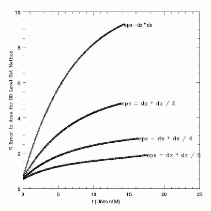
FIG. 1.: Percent error in area of $M=2$, $a=0$ event horizons in survey over viscosity parameter: $\epsilon=$ $h^{2}$, ${h^{2}}/2$, ${h^{2}}/4$, ${h^{2}}/8$. Here increasing $t$ corresponds to propagation into the past.

In figures (1) -(4) we show the evolution backward in time of the eikonal equation (followed by extraction of the $S=0$ surface). Errors can arise both in the evolution and in the extraction of the surface. Figure (1) shows the percent errors in the extracted areas for a nonspinning black holes with mass $M=2$, $a=0$ in a survey over the viscosity parameter. Figure (2) shows a similar study but for the L2 norm of the truncation error in the function $r_{+}$. Note that the function $r_{+}$ is defined for every point of the horizon in the continuum $r_{+}=r_{+}\left(x,y,z\right)$. In the computational domain $r_{+}$ then takes a discrete form $\hat{r}_{+}=\hat{r}_{+}\left(i,j,k\right)$, where the integers $i,j,k$ span the numerical mesh. The truncation error $e_{r_{+}}$ is then

$$e_{r_{+}}\left(i,j,k\right)=r_{+}\left(x,y,z\right)-\hat{r}_{+}\left(i,j,k\right)$$ (62)

where is it understood that both $r_{+}$ and $\hat{r}_{+}$ are evaluated at the same point. Bith Figures(1) and (2)show that viscosity parameter $h^{2}/8$ adequately captures the horizon location. While not perfect, it will suffice for the short term horizon tracking reported here.

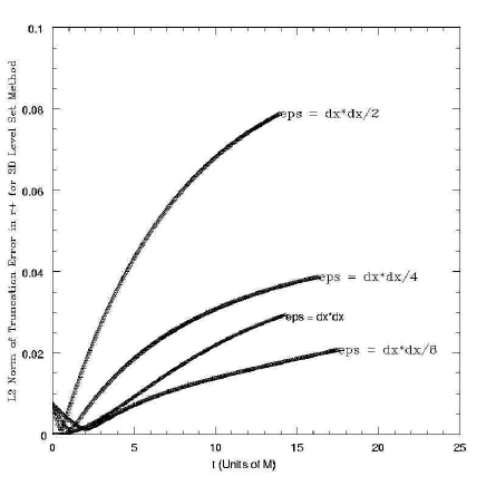
FIG. 2.: L2 norm in truncation error of $r_{+}$ for $M=2$, $a=0$ event horizons in survey over viscosity parameter: $\epsilon=$ $h^{2}$, ${h^{2}}/2$, ${h^{2}}/4$, ${h^{2}}/8$. Here increasing $t$ corresponds to propagation into the past.

However these results also suggest that in vanishing viscosity the percentage error in the calculated area is reduced toward a bias. This bias is partly associated to the finite resolution of the computational mesh and partly to accuracy of the extraction routine. These figures were generated using a three dimensional computational domain of $N^{3}$ points with $N=121$. The outer boundaries are located at $\left[-15M,+15M\right]$ in the $x,y,z$ directions. The resolution of the finite difference mesh for these results is then $h=M/4$. Also, a Courant - Friedrichs - Lewy factor of $\lambda=1/4$ with an iterated Crank Nicholson scheme [22] was used as the finite difference approximation of the evolution of the eikonal equation (18). Neumann boundary conditions $\partial_{i}S=0$ on the outer boundary are found to be generically sufficient conditions for stability of the method. The philosophy here is that the primary interest is deep within the bulk of the computational domain where the event horizon of the black hole is located. The outer boundary is then treated only to the degree that the evolution of the interior region remains stable. Further, the interior of the black hole is excised from the computational domain in a sphere of radius $r=r_{0}+2dx$, where $r_{0}$ denotes the radius of the Kerr - Newman ring curvature singularity. Finally, the discrete surface $\hat{\Gamma}$ was constructed using $m^{2}$ points with $m=100$. At such a resolution of the extracted surface any errors in the area must be attributed to all of: the viscosity parameter, the extraction routine, and the resolution of the underlying three dimensional grid.

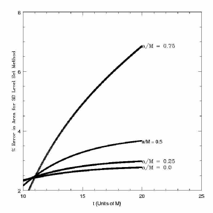
FIG. 3.: Percent error in area for three dimensional level set solutions $a/M=$, $0$, $1/4$, $1/2$, $3/4$. Here increasing $t$ corresponds to propagation into the past.

Figures (3) and (4) show the percent errors in the extracted areas as well as the L2 Norm of the truncation error in the function $r_{+}$ in a survey over the angular momentum parameter $a$. Here the viscosity is $\epsilon=h^{2}$. These figures both show the evolution from a single null sphere that is completely exterior to the horizon and propagated into the past. Since the event horizon of a spinning black hole is elliptical in its geometry, the spherical data we have chosen for $t_{\downarrow}=0$ corresponds to a percent error in the area and $r_{+}$ that varies with the spin parameter $a/M$ at $t_{\downarrow}=0$, explaining why the curves do not intersect at $t_{\downarrow}=0$. (Where appropriate we append a $\downarrow$ to $t$, thus: $t_{\downarrow}$, indicating evolution into the past; we also sometimes use $t_{\uparrow}$ to emphasize that we mean the forward evolving, usual, time $t$. Thus $t_{\downarrow}=0$ corresponds to the late time at which we begin to integrate into the past.)

However, the errors should converge to a constant, which is evident in each of the curves with $a<0.75$ in figures (3) and (4). For $a=0.75$ the curve does not converge, and we expect that different choice of initial data will exhibit convergence. According to these results, the viscosity level set method does indeed accurately and robustly detect the distorted outermost event horizons of spinning black holes at least when $a<0.75$. Note that we study both the accuracy of $r_{+}$ and the accuracy of the calculated areas since the calculations seperately and together establish the accuracy of our area calculation and of our detection of the event horizon.

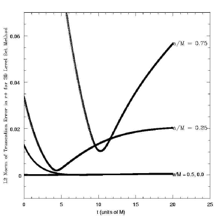
FIG. 4.: L2 norm of truncation error in $r_{+}$ for three dimensional level set solutions $a/M=$ $0$, $1/4$, $1/2$, $3/4$. Here increasing $t$ corresponds to propagation into the past.

V Asymmetric Binary Black Hole Coalescence

Analysis of the event horizon for the binary black hole coalescence problem in the case of head on collision has been considered in detail in [16]. The problem of the event horizon for asymmetric, that is off axis, collision has only been considered analytically [23] and prior to this work no results for numerically generated sources have been analyzed. Numerical evolution and analysis of an asymmetric binary black hole system was studied in [24], but at that time the question of the event horizon was not considered.

In this section the results of the previous sections are applied to the first completely numerical analysis of the event horizon for the case of asymmetric collision.

To begin, consider two black holes of mass $M=1$ with aligned spins in the positive $z$ direction of $a/M=1/2$. The computational domain is a grid of $N^{3}$ points with $N=121$. The outer boundary is located at $\pm 15M$ and the holes are initially positioned at $\left(x,y,z\right)=\left(+6,+2,0\right)$, and $\left(x,y,z\right)=\left(-6,-2,0\right)$. This computational domain is identical to the mesh used in the previous section to analyze the percent error in area calculations of surfaces extracted from the level set method. The percent error in the calculation of the area of sections of the horizon should have a magnitude of about $4-5\%$. Further, as an order of magnitude estimate, in a flat spatial geometry; e.g., in a Newtonian spacetime, the initial separation $s$ of the black hole centers would be $s=\sqrt{12^{2}+4^{2}}\approx 12.64$. This would seem to be an ample initial separation to guarantee that the initial data corresponds to two distinct black holes. However, in the case that the holes are nonspinning, each will have a spherical event horizon of radius $r=2M$. Assuming only marginal distortion of the nonspinning event horizons due to spin effects, which is an approximation that is justified by the properties of spin $a/M=1/2$ black holes, the nearest separation between the two sections of the black hole event horizon is then approximately $s_{min}=12.64M-4M\approx 8.64M$. Again, this approximation assumes a flat underlying geometry; and so can be considered only as an order of magnitude estimate. These initial data then appear to correspond to a separation of approximately two nonspinning black hole diameters between the surfaces of section of the black holes.

The holes are boosted along the $x$ direction with speeds of $\pm c/2$. This boost lengthens the nearest separation $s_{min}$ of the holes due to Lorentz contraction of the horizons.[In this coordinate system the horizons undergo contraction in the direction of motion. For a single hole, the area of the horizon does not change under this boost.] The nearest coordinate separation $s_{min}$ between the holes is then expected to lie in the range $8.64<s_{min}<12.64$.

The numerical evolution of this collision process is carried out for approximately $10M$ of run time with a Courant factor of $\lambda=dt/dx=1/4$. The code is the Texas black hole evolution code, a derivative of the Agave code [24]. Apparent horizon finders [25] locate two distinct apparent horizons of area $A\approx 50M$ for the initial data and continue to do so until $t=8M$, when only a single apparent horizon of area $A\approx 200M$ can be located. This single apparent horizon persists until approximately $10M$, beyond which instability effects, stemming from the outer boundary and the excision boundary, swamp the solution.

VI Data For the Eikonal

While the run length of this asymmetric collision data is relatively small in units of the black hole masses, the problem of detecting the associated black hole event horizon, or horizons, is not a small computational problem. For example, to analyze this data requires analysis of the lapse $\alpha$, the shift vector $\beta^{i}$, and the three metric $\gamma^{ij}$. By symmetry of the metric, $\gamma^{ij}=\gamma^{ji}$, there are only 6 independent components. Tracking the event horizon of the associated data then requires analysis of 10 grid functions, where each grid function consists of ${\mathcal{O}}\left(Nt\times N^{3}\right)\times 8B={\mathcal{O}}\left(160\times 121^{3}\right)\times 8B\approx 2.26GB$ of data. That is, tracking the associated event horizon requires analysis of approximately $20GB$ of data.

A more serious difficulty associated to this data set is the relaxation time, $t\approx 4M$, that is typically required for outgoing data to converge onto the event horizon when followed into the past. Assuming that the collision time is (as suggested by the apparent horizon solvers) near $t=8M$, perturbation theory implies that the resulting horizon should undergo quasi normal ringing for another $t\approx 20M$ from that time. That is, at the time level $t=10M$, where the event horizon tracker will begin tracking into the past, it is expected that the event horizon remains highly distorted and far from its stationary regime. The problem is to determine good data for the eikonal at the time level $t=10M$, which can then be propagated into the past. In contrast, in analysis of the event horizon for the case of head on collision, researchers made use of approximately $100M$ of data [16], and assumed that the final state at $t=100M$ was a stationary or quasi stationary black hole. In such a circumstance using spherically symmetric data at $t=100M$ for an event horizon tracking method should prove sufficient. The difficulty with a data set only of length $t=10M$ is that using spherically symmetric data for the eikonal at the time level $t=10M$ does not accurately approximate sections of the event horizon at that time.

To accommodate data of this $10M$ length and to generate sufficient data for the eikonal at the time level $t=10M$, a method for finding a candidate section of the event horizon at $t=10M$ is proposed here and applied to the problem. This method makes use of the analytic properties of apparent and event horizons.

To motivate the method, note that if the event horizon were stationary at $t=10M$ then the expansion of the surface would be vanishing there:

$$\theta\left(t=10M\right)=\frac{1}{A}\frac{dA}{dt}=0.$$ (63)

In such a circumstance the apparent horizon could be used as initial data for the eikonal, which could then be propagated into the past. However, according to the second law of black hole mechanics, in the case that the horizon is nonstationary, which is the situation expected for this asymmetric problem, at $t=10M$ the horizon will satisfy

$$\theta\left(t=10M\right)\geq 0,$$ (64)

in the forward time direction. In the backwards time direction these dynamics correspond to $\theta\leq 0$ at $t=10M$. As such, the Taylor series of any compact null surface, including the critical surface of the event horizon, is at least of the form

$$A\left(t+dt\right)=A\left(t\right)+dtA\theta+dt^{2}\frac{d^{2}A}{2dt^{2}}+\ldots$$ (65)

and probably cannot be truncated to below

$$A\left(t+dt\right)\approx A\left(t\right)+dtA\theta+\ldots$$ (66)

The apparent horizon is then a poor estimate for the the event horizon at $t=10M$. The objective is to use this behavior (66) in combination with the property that outgoing null data followed into the past converges to the event horizon. The hope is to establish a better approximation for the structure of the section of the event horizon at $t=10M$, which can then be used in an event horizon tracking method.

To proceed, consider three compact null surfaces of outgoing data: One completely interior to the horizon $\Gamma^{i}$, one completely exterior to the horizon $\Gamma^{e}$, and one that is a surface of section of the event horizon $\Gamma^{h}$. Let $t_{\downarrow}\rightarrow\infty$ denote propagation into the past. By the property that outgoing data numerically converges to the horizon when propagated into the past, $\lim_{t_{\downarrow}\rightarrow\infty}\Gamma^{i}=\lim_{t_{\downarrow}\rightarrow\infty}\Gamma^{e}=\lim_{t_{\downarrow}\rightarrow\infty}\Gamma^{h}$. Thus in most cases, if the surface $\Gamma^{i}\left(t_{\downarrow}+dt_{\downarrow}\right)$ is pulled back to the time level $t_{\downarrow}$ and compared to the surface $\Gamma^{i}\left(t_{\downarrow}\right)$ it will be completely exterior to $\Gamma^{i}\left(t_{\downarrow}\right)$. Similarly, if the surface $\Gamma^{e}\left(t_{\downarrow}+dt_{\downarrow}\right)$ is pulled back to the time level $t_{\downarrow}$ it will be completely interior to the surface $\Gamma^{e}\left(t_{\downarrow}\right)$. That is, by iteratively pulling the surfaces back to a single time level, spherically symmetric data will approach the numerical event horizon. Exceptions to this general behavior stem from the presence of caustics in the spacetime, where null surfaces intersect, and in neighborhoods of the event horizon. In particular, as discussed above, the horizon of this asymmetric collision data is expected to satisfy $\theta\geq 0$. If the surface $\Gamma^{h}\left(t_{\downarrow}+dt_{\downarrow}\right)$ is then pulled back to $t_{\downarrow}$ it will be interior to the surface $\Gamma^{h}\left(t_{\downarrow}\right)$. Let $\Gamma^{i}_{\epsilon}\left(t_{\downarrow}\right)$ be a perturbation of $\Gamma^{h}\left(t_{\downarrow}\right)$ that is arbitrarily close to the horizon $\Gamma^{h}\left(t_{\downarrow}\right)$ but completely interior to the surface $\Gamma^{h}\left(t_{\downarrow}\right)$. Due to round off and truncation error of the finite difference approximation and the fact that $\lim_{t_{\downarrow}\rightarrow\infty}\Gamma^{i}_{\epsilon}=\Gamma^{h}$, if the numerical finite difference approximation $\hat{\Gamma}^{i}_{\epsilon}\left(t_{\downarrow}+dt_{\downarrow}\right)$, which approximates the continuum section $\Gamma^{i}_{\epsilon}\left(t_{\downarrow}+dt_{\downarrow}\right)$, is pulled back to the time level $t_{\downarrow}$ it will generically intersect $\hat{\Gamma}^{i}_{\epsilon}\left(t_{\downarrow}\right)$ and contain neighborhoods that are both interior and exterior to the finite difference approximation $\hat{\Gamma}^{i}_{\epsilon}\left(t_{\downarrow}\right)$. Similar behavior will hold for numerical data $\hat{\Gamma}^{e}_{\epsilon}\left(t_{\downarrow}\right)$ defined to be a perturbation of $\hat{\Gamma}^{h}\left(t_{\downarrow}\right)$ that is arbitrarily close to the horizon $\hat{\Gamma}^{h}\left(t_{\downarrow}\right)$ , and completely exterior to $\hat{\Gamma}^{h}\left(t_{\downarrow}\right)$.

According to this behavior, data for the eikonal at the time level $t=10M$ can be constructed by iteration over that time slice. This approach is similar to treating the event horizon as if it were an apparent horizon, although modified to account for this nonstationary regime. Beginning with spherically symmetric initial data that is well exterior to the horizon $\hat{\Gamma}^{e}_{1}\left(t_{\downarrow}=10M\right)$ the data is updated, pulled back to the original time level and reset as follows: $\hat{\Gamma}^{e}_{2}\left(t_{\downarrow}\right)=\hat{\Gamma}^{e}_{1}\left(t_{\downarrow}+dt_{\downarrow}\right)$. The step $\hat{\Gamma}^{e}_{n+1}\left(t_{\downarrow}\right)=\hat{\Gamma}^{e}_{n}\left(t_{\downarrow}+dt_{\downarrow}\right)$ is then repeated for several hundred iterations, which corresponds to ${\mathcal{O}}\left(10\right)$ $e$ folding times. Note that in the case that the spacetime is stationary the surface $\hat{\Gamma}$ will converge to the apparent horizon according to this method. Since the apparent horizon of a stationary spacetime coincides with the event horizon, this method will generically find the event horizon in the case of stationary spacetimes. However, in the nonstationary regime, which is the case for the asymmetric collision problem, the result of this procedure is at best an improved initial guess for an event horizon tracker. Further information, such as area analysis or study of the apparent horizon, is required to argue that the resulting surface is a candidate section of the event horizon.

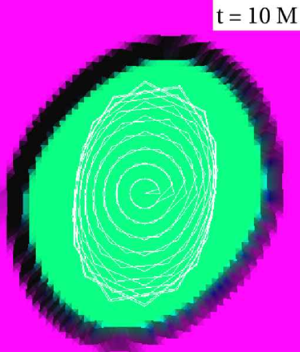
FIG. 5.: Tanh data (see Eq(67) for the eikonal in asymmetric binary black hole coalescence. The black contour is the estimate of the event horizon section, while the wire mesh is the apparent horizon. These data are set at the end of the computational evolution ($t=10M$), and will be evolved into the past.

We show in figure (5) the result of such a process, applying $\approx 200$ iterations over the time slice $t=10M$. Figures (5) through (11) show the eikonal function in the $z=0$ plane. The location of the determined guess for the surface $\Gamma$ (which we will take to begin our evolution of the horizon into the past) is encoded into the eikonal by the color map. With this $\Gamma$, data for the eikonal can be written in the form:

$$S\left(0,x^{i}\right)=1+\tanh\left(\frac{r_{c}-r}{c}\right)$$ (67)

In equation (67) the first argument of the eikonal is $t_{\downarrow}=0$; $t_{\downarrow}$ will increase into the past. Also, $r_{c}$ denotes the data $\Gamma$ and $c$ controls its steepness. Typically we take a transition width $c$ on the order of a computational zone. Note that this surface is not considered to be a true section of the event horizon, but instead is a good initial guess or candidate section, which after a few $M$ will evolve into better approximation of a true section of the event horizon. By way of comparison figure (5) also shows at $t=10M$ the final apparent horizon as a white wire mesh. Note that both the apparent horizon and these data for the eikonal are highly distorted from the stationary case. Figure (6) shows the resulting eikonal function $S\left(x,y,z\right)$ after $2M$ of evolution into the past. Note that the surface $\Gamma$ is not qualitatively changed during the evolution.

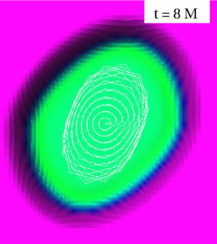
FIG. 6.: Data of figure (5) (asymmetric binary black hole coalescence) evolved backward from $t=10M$ to $t=8M$.

VII Surface Extraction and Apparent Horizons

Figure (7) shows several frames of the evolution of the eikonal using a viscosity solution of $\epsilon=h^{2}$ (not of the improved viscosity form). This figure display the value of the eikonal function on the $z=0$ plane. Figure (7) shows the eikonal data as an elevation map and also via the color map of (5). Note in those figures that null surfaces interior to the event horizon undergo a change in topology and this topological transition is continuously monitored by the viscosity solutions of the eikonal. In figure (7) $t=0.562M$ is shown in the upper left-hand corner, $t=1.5M$ is shown in the upper right-hand corner, $t=2.5M$ is shown in the lower left-hand corner and $t=5.0M$ appears in the lower right-hand corner.

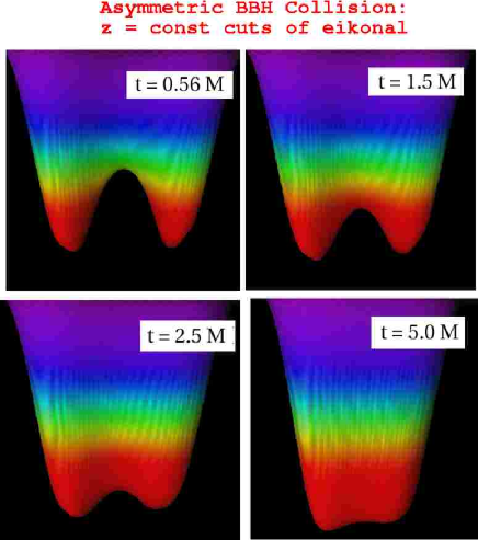
FIG. 7.: Change of topology in eikonal for asymmetric binary black hole coalescence, shown as an elevation map.

The figures (8) - (11) continue the sequence of figures (5) - (6), and show, for several values of $t_{\uparrow}$, the value of the eikonal in the $z=0$ plane; the location of the apparent horizon in the $3$ dimensions (the white wire frame); and in the black wire frame, locations of sections of a candidate event horizon $\hat{\Gamma}_{c}\left(t_{\downarrow}\right)$ that is generated by evolution of the eikonal equation from data constructed using the method described in the previous section. In this context, the surfaces $\hat{\Gamma}_{c}\left(t_{\downarrow}\right)$ are extracted from the eikonal data using the technique described in section IV. Note that $\hat{\Gamma}_{c}$ completely contains the apparent horizons throughout their evolution. This is a fundamental condition that any numerically constructed black hole event horizon must satisfy. To determine how these results depend on the initial data $\hat{\Gamma}_{c}\left(t_{\downarrow}=0\right)$, choosing initial data $\hat{\Gamma}_{\delta}\left(t_{\downarrow}=0\right)$ of the form

$$u_{\delta}\left(\theta,\phi\right)=u_{c}\left(\theta,\phi\right)-\delta,$$ (68)

permits survey about the data $u_{c}\left(\theta,\phi\right)$, where $u_{c}\left(\theta,\phi\right)$ corresponds to the data $\hat{\Gamma}_{c}\left(t_{\downarrow}=0\right)$. Studies with $\delta=M/2,M,2M$ establish that the level sets $\hat{\Gamma}_{\delta}$ penetrate both apparent horizons for any $\delta\geq M/2$. These results suggest that the true event horizon is contained in a domain parameterized by $0<\delta<M/2$.

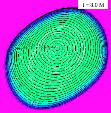
FIG. 8.: Asymmetric binary black hole coalescence: $t_{\uparrow}=8M$. This is the same as figure (6) but the black wire mesh shows the estimated location of the event horizon.

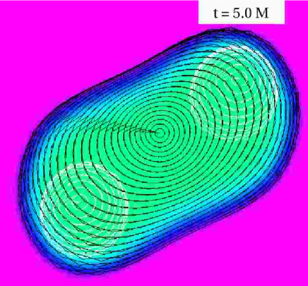
FIG. 9.: Asymmetric binary black hole coalescence: $t_{\uparrow}=5M$. Note that while the apparent horizons (the white wire-frame “spheres”) are still well separate at $t=5M$, the event horizon (black wire frame “peanut” already has one component only.

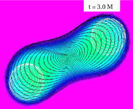
FIG. 10.: Asymmetric binary black hole coalescence: $t_{\uparrow}=3M$.

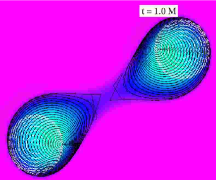
FIG. 11.: Asymmetric binary black hole coalescence: $t_{\uparrow}=1M$. Careful inspection of the event horizon (black wireframe) suggests two separated components.

Figures (12) and (13) show two views of the extracted level set $S=0$ at $t=2M$. Note that this surface is highly distorted and shows the event horizon just after merger. Also shown in these figures are the apparent horizons for the two black holes. In these figures each color of the color map denotes a level set $\hat{\Gamma}$ of the eikonal. As such, each color represents a null surface. From these figures it is apparent that at this time there appears one innermost null surface that completely contains both apparent horizons. Thus, the results of the viscosity solutions suggest a merger time much closer to $2M$ then the $8M$ found with the apparent horizon trackers. [Note that in figures (12) and (13) the event horizon is shown as a white wire mesh, while the apparent horizons are shown as black wire meshes. This is opposite to the color scheme used in figures 5, 6, 8 - 11, which was an independent study of the evolution as opposed to the study of the throat geometry considered here.]

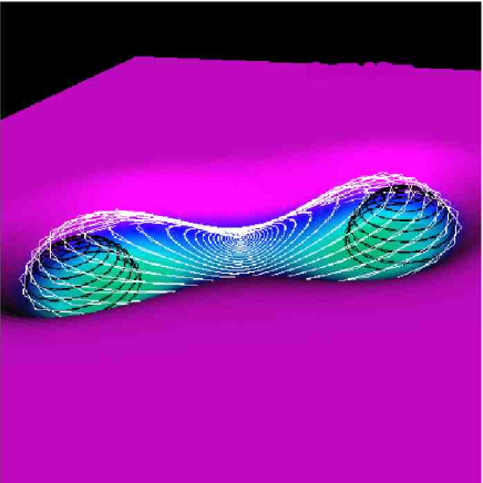
FIG. 12.: Level set extraction for asymmetric binary black hole coalescence: I.

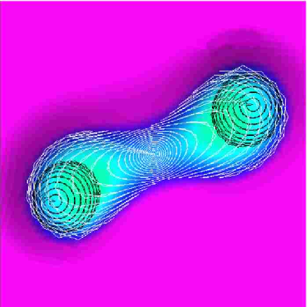
FIG. 13.: Level set extraction for asymmetric binary black hole coalescence: II.

VIII Change of Topology

As shown in figure (7) the viscosity solutions of the eikonal equation do continuously monitor a change in topology. In the case of asymmetric binary black hole coalescence it is conjectured that the level set $\Gamma$, which corresponds to a section of the event horizon, must take a higher genus topology at merger. To investigate this possibility, figure (14) shows the level set $\hat{\Gamma}$ viewed along the axis joining the centers of the apparent horizons. In that figure it is apparent that the throat function of the topological transition is elliptical in geometry. Studies indicate that this elliptical throat function persists for all null surfaces (i.e. those slightly inside or slightly outside our candidate event horizon) undergoing the topological transition. Further, for all of our computed transitions of the null surfaces, no higher genus topology is exhibited; instead, the elliptical geometry of the throat persists to the transition. These results suggest that if there is a non trivial topology in the sections of the event horizon as a consequence of the asymmetry of the merger, then that topology change is bounded to occur when the minor axis of the ellipse is within one of our computational zones, or $h=M/4$.

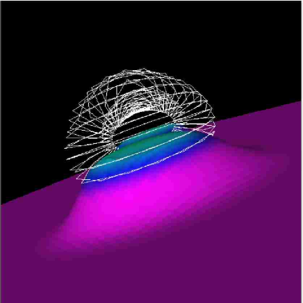
FIG. 14.: Throat function for asymmetric binary black hole coalescence: $t_{\uparrow}=1.562M$.

IX Area Analysis

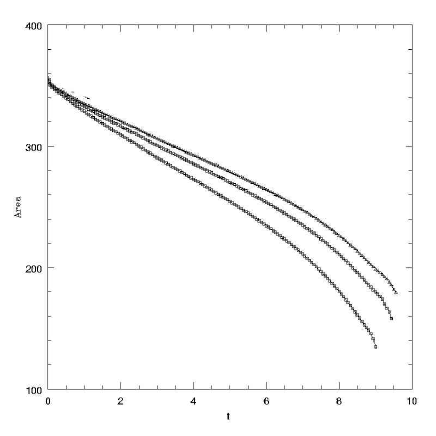
FIG. 15.: Area versus time for asymmetric binary black hole coalescence.The horizontal scale is $t_{\downarrow}$, i.e. time measured into the past. The curves are (bottom to top) for $\epsilon=2h^{2}$, $\epsilon=h^{2}$, and the improved viscosity solution.

X Black Hole Areas

Figure (15) shows an area versus time plot for this asymmetric collision. The curve with the lowest area is the result of a viscosity solution with $\epsilon=2h^{2}$. The curve with the second lowest area is the result of a viscosity solution with $\epsilon=h^{2}$, while the topmost curve is an improved viscosity solution composed of the two higher viscosity solutions. According to these results it is immediately apparent that the viscosity solutions of higher viscosity show a merger time that is later in $t_{\uparrow}$ (and therefore prior in $t_{\downarrow}$) then the merger time found with solutions constructed in the limit of vanishing viscosity. These results then indicate that the error (or bias) in the merger time of the viscosity solutions is directly related to the magnitude of the viscosity. More precisely, for the continuum merger time of $t^{*}_{\uparrow}$ and an approximate merger time of ${t^{*}_{\uparrow}}_{\epsilon}$, constructed using a viscosity solution of viscosity parameter $\epsilon$, the function $f\left(\epsilon\right)={t^{*}_{\uparrow}}_{\epsilon}-t^{*}_{\uparrow}$ is increasing in $\epsilon$. (Here all surface areas are calculated with $m^{2}$ points where $m=100$.)

FIG. 16.: Areas versus time for asymmetric binary black hole coalescence. The horizontal scale is $t_{\downarrow}$.

Figure (16) shows several area versus time curves for initial data of the form

$$u_{\delta}\left(\theta,\phi\right)=u_{c}\left(\theta,\phi\right)-\delta$$ (69)

where the data $u_{c}\left(\theta,\phi\right)$ is that obtained using the method of section VII. From top to bottom, the curves show areas for $\delta=0,M/4,M/2$ and with a viscosity parameter of $\epsilon=h^{2}$. Recall that studies of the apparent horizons found that the true event horizon is contained in the domain $0<\delta<M/2$. This survey over $\delta$ is conducted in search for the convergence signature associated to event horizons. Due to the time scale of this data, the time scale of the dynamics, and the relaxation time scale of the event horizon tracking method, the signature is not clearly apparent. However, this study of the area curves does show convergence of the areas, which is expected for null data approaching the horizon when propagated into the past. The curve with $\delta=M/2$ shows behavior suggestive of an event horizon since the $\delta\neq M/2$ curves all approach that of $\delta=M/2$. The $\delta=M/2$ curve is therefore considered the best candidate for the numerical event horizon of this study. Note that the sections of this event horizon completely contain the correct apparent horizons for all $t_{\downarrow}<9M$. Further, these $\delta=M/2$ data show a bifurcation time at $t_{\downarrow}\approx 8.3M$, which corresponds to a merger time of about $t_{\uparrow}\approx 1.7M$. This bifurcation time is detected by an algorithm that searches for any points $\theta,\phi$ of the surface such that $u\left(\theta,\phi\right)<h$. In the circumstance that a point is found such that $u\left(\theta,\phi\right)<h$, the bifurcation is expected to occur in a few more $dt=M/16$ in the $t_{\downarrow}$ direction. A few time levels prior to this bifurcation time in $t_{\downarrow}$ (i.e. just after the bifurcation in $t$), the single merged horizon component has an area (the area of the level set) computed to be $A=148.9$. Based on analysis of area computations for exact solutions (figure(3), we anticipate an error in the horizon area of several percent. We conservatively assign an $8\%$ error to the areas. Just prior (in $t$) to merger the area of each black hole is then $A=74.5\pm 6.0M^{2}$. These individual areas correspond to a Schwarzschild mass of about $M=1.48\pm 0.12$. This result is a substantially larger mass for each hole then determined by the apparent horizon finders at the time level $t_{\uparrow}=0$. Interestingly, studies have found that apparent horizons separated by about $10M$ show an increase in their mass due to the effects of binding energy[26]. Individual masses of about $M\approx 1.36$ are then only a slight departure from studies that account for the binding energy of the holes. Further, at the time of merger the holes have undergone $1.7M$ of evolution, during which the holes could accrete any surrounding gravitational radiation present in the initial data. The presence of such radiation would lead to larger masses then those found using apparent horizon finders at $t_{\uparrow}=0$. However, it is important to note that due to the viscosity in the solution the result $M\approx 1.36$ can only properly be considered as a lower bound on the calculated masses. The most significant contribution to any error in this result must stem from the relatively small time scale of this asymmetric collision data and coupling of that time scale to the $e-$folding time scale of this event horizon detection method.

XI Conclusions

In this work we have demonstrated a relatively simple yet robust and (most importantly) generic solution to the problem of numerically tracking black hole event horizons. An implementation of our method made use of an explicit second order diffusion term to regulate the solution singularities associated to caustics. As demonstrated by analysis of analytic sources, this term does introduce numerical error although we demonstrate our control over these effects and the resulting accuracy. But, the use of a second order diffusion term is not required by our method per se; and a variety of other approaches can be employed. Examples of other methods for controlling breakdown of the numerical solution include those classes of high resolution shock capturing numerical schemes that are used extensively in computational fluid dynamics for hyperbolic problems similar to the eikonal equation.

The application of our new method for event horizon tracking method considered the asymmetric binary black hole coalescence problem, including a detailed analysis of areas of the surfaces of sections, the collision time, associated apparent horizons, and the topology of the horizon. Due to the relatively short time scale of the collision data, our method was unable to demonstrate the signature of the black hole event horizon. We believe that this problem is due to the data itself and not due to our method. We anticipate much more accurate and convincing results as more accurate computational simulations of black hole interactions become available.

REFERENCES

- [1] S. W. Hawking and G. F. R. Ellis, “The Large Scale Structure of Spacetime”, Cambridge University Press(1973).
- [2] J. R. Oppenheimer and H. Snyder, Phys. Rev., 56, 455 (1939).
- [3] B. Carter,, Phys. Rev. Lett., 26, 331 (1971).
- [4] J. M. Bardeen, B.Carter, and S. W. Hawking, Commun. Math. Phys., 31, 161 (1973).
- [5] R. M. Wald, “Quantum Field Theory in Curved Spacetime and Black Hole Thermodynamics”, University of Chicago Press (1994).
- [6] M. W. Choptuik, Phys. Rev. Lett., 70, 9 (1993).
- [7] A. Celotti, J. C. Miller, and D. W. Sciama, Class. Quant. Grav., 16, 3 (1999).
- [8] K. Menou, E. Quataert, and R. Narayan, Proc. Marcel Grossmann Meeting on General Relavity, (1997).
- [9] Richstone et al, Nature, 395, A14 (1998).
- [10] K. Belczynski, V. Kalogera, and T. Bulik, Astrophys. J., 572, 407 (2001).
- [11] L. Lehner, Class. Quantum. Grav., 18, 161 (2001).
- [12] L. P. Grischuk et al, Physics-Uspekhi, 171, 3 (2001).
- [13] S. A. Hughes et al, Phys. Rev D., 49, 4004 (1994).
- [14] P. Anninos et al, Phys. Rev Lett., 74, 630 (1995).
- [15] R. A. Matzner et al, Science, 270, 941 (1995).
- [16] J. Libson et al, Phys. Rev. D., 53, 4335 (1996).
- [17] J. Masso et al, Phys. Rev. D., 59, (1999).
- [18] A. Ashtekar et al, Phys. Rev. Lett., 85, 3564 (2000).
- [19] J. Ehlers and E. T. Newman, J. Math. Phys., 41, 3344 (2000).
- [20] S. Frittelli and E. T. Newman, J. Math. Phys., 40, 383 (1999).
- [21] E. T. Newman and A. Perez, J. Math. Phys., 40, 1093 (1999).
- [22] S. A. Teukolsky, Phys. Rev. D, 61, 087501 (2000).
- [23] S. Husa and J. Winicour, Phys. Rev D., 60, 84019 (1999).
- [24] S. Brandt et al, Phys. Rev. Lett., 85, 5496 (2000).
- [25] D. M. Shoemaker, M. F. Huq, and R. A. Matzner, Phys. Rev. D, 62, 124005 (2000).
- [26] E. Bonning, D. Neilsen, and Richard A. Matzner, ”Physics an dInitial Data for Black Hole Spacetimes”, in preparation (2003).