A scalar hyperbolic equation
with GR-type non-linearity

Abstract

We study a scalar hyperbolic partial differential equation with non-linear terms similar to those of the equations of general relativity. The equation has a number of non-trivial analytical solutions whose existence rely on a delicate balance between linear and non-linear terms. We formulate two classes of second-order accurate central-difference schemes, CFLN and MOL, for numerical integration of this equation. Solutions produced by the schemes converge to exact solutions at any fixed time $t$ when numerical resolution is increased. However, in certain cases integration becomes asymptotically unstable when $t$ is increased and resolution is kept fixed. This behavior is caused by subtle changes in the balance between linear and non-linear terms when the equation is discretized in space. Changes in the balance occur without violating a second-order accuracy of the discretization. We thus demonstrate that second-order accuracy and convergence at finite $t$ does not guarantee a correct asymptotic behavior and long-term numerical stability. Accuracy and long-term stability of integration are greatly improved by an exponential transformation of the unknown variable.

1 Introduction

It is well known that numerical integration of Einstein’s equations in a 3+1 form often leads to instabilities and terminates prematurely. Some of the instabilities have been related to the presence of constraints, and some to the existence of gauge degrees of freedom in Einstein’s equations ([1],[2], and references therein). These instabilities are intrinsic to the equations of general relativity (GR) themselves. Numerical instabilities may also arise due to a bad choice of a finite-difference scheme.

In this paper we introduce a scalar hyperbolic partial differential equation with non-linear terms similar to those of much more complicated equations of GR (Section 2). The equation has a number of non-trivial analytical solutions (Sections 3 and 4). We experiment with several finite-difference schemes for numerical integration of this equation (Section 5).

Solutions produced by the schemes converge to exact solutions at any fixed moment of time $t$ when numerical resolution is increased. However, in certain cases numerical integration becomes unstable when $t$ is increased while the resolution is kept fixed (Section 6). We trace this behavior to a special structure of the non-linear terms and demonstrate that discretization of non-linear terms leads to a finite-difference system whose asymptotic behavior may differ qualitatively from the corresponding behavior of a continuous system (Section 7). The accuracy and stability of integration can be greatly improved by an exponential transformation of the unknown variable (Section 7).

2 A model equation

Consider a scalar, quasi-linear, hyperbolic partial differential equation of two independent variables, $t$ and $x$,

$$a_{11}g_{tt}+2a_{12}g_{tx}+a_{22}g_{xx}+g^{-1}(b_{11}g_{t}^{2}+2b_{12}g_{t}g_{x}+b_{22}g_{x}^{2})=0,$$ (2.1)

where $g=g(t,x)$ is the unknown, and $a_{ij}$, $b_{ij}$ are constant coefficients, $a_{11}a_{22}-a_{21}^{2}<0$. The non-linear term in (2.1) has the form $g^{-1}\,\sum\text{(first derivatives squared)}$.

The reason for considering (2.1) becomes obvious if we recall that the structure of a Ricci tensor $R_{ab}$ is $R\sim\sum\partial\Gamma+\sum\Gamma\Gamma$, where Cristoffel symbols $\Gamma\sim g^{-1}\partial g$, and $g$ is the metric. Thus, $R_{ab}$ is represented as a sum of the terms $R\sim\sum g^{-1}\partial^{2}g+\sum g^{-2}(\partial g)^{2}$. Equation (2.1) thus mimics a type of non-linearity present in GR equations $R_{ab}=0$. In particular, (2.1) may have a singularity related to $g$ becoming zero.

Equation (2.1) can be reduced to its normal form,

$$g_{tt}=g_{xx}-g^{-1}(\alpha g_{t}^{2}+\beta g_{x}^{2}+\gamma g_{x}g_{t}),$$ (2.2)

by a linear transformation which preserves a quadratic form of the non-linearity. We work below with a simpler equation (2.2). This is a non-linear hyperbolic equation with a characteristic speed equal to $1$.

By introducing a new variable $K=g_{t}$, we rewrite (2.2) as a system of two first-order in time partial differential equations

$$\begin{split}&g_{t}=K,\\ &K_{t}=g_{xx}-g^{-1}(\alpha K^{2}+\beta g_{x}^{2}+\gamma Kg_{x})\\ \end{split}$$ (2.3)

which resembles the evolutionary part of GR equations in a standard ADM 3+1 form (with zero shift and constant lapse). By introducing yet another variable $D=g_{x}$ we further rewrite (2.2) as a system of first-order PDE

$$\begin{split}g_{t}&=K,\\ K_{t}-D_{x}&=R,\\ D_{t}-K_{x}&=0,\\ \end{split}$$ (2.4)

where

$$R\equiv-g^{-1}(\alpha K^{2}+\beta D^{2}+\gamma DK).$$ (2.5)

This system has a complete set of real eigenvalues and eigenvectors.

3 Exponential transformation

A transformation

$$g=e^{\phi},$$ (3.1)

where $\phi$ is a new unknown, will play an important role in subsequent sections. After substitution of (3.1) into (2.2) we obtain a PDE for a new unknown $\phi$,

$$\phi_{tt}=\phi_{xx}-(\alpha+1)\phi_{t}^{2}-(\beta-1)\phi_{x}^{2}-\gamma\phi_{x}\phi_{t}.$$ (3.2)

The transformation (3.1) removes $g^{-1}$ multiplier in front of the non-linear term in (2.2), and maps $0<g<\infty$ onto $-\infty<\phi<\infty$ so that values of $g\leq 0$ are excluded. This is consistent with GR where three-dimensional metric of space-like hypersurfaces is positive-definite.

We can introduce new variables

$$\psi\equiv\phi_{t},\quad\theta\equiv\phi_{x},$$ (3.3)

and rewrite (3.2) in the equivalent two-equation form similar to (2.3) as

$$\begin{split}\phi_{t}&=\psi,\\ \psi_{t}&=\phi_{xx}-(\alpha+1)\psi^{2}-(\beta-1)\phi_{x}^{2}-\gamma\psi\phi_{x},\\ \end{split}$$ (3.4)

or in a three-equation form similar to (2.4) as

$$\begin{split}\phi_{t}&=\psi,\\ \psi_{t}-\theta_{x}&=S,\\ \theta_{t}-\psi_{x}&=0,\\ \end{split}$$ (3.5)

where

$$S=-(\alpha+1)\psi^{2}-(\beta-1)\theta^{2}-\gamma\psi\theta.$$ (3.6)

System (3.5)obviously has the same eigenvectors and eigenvalues as (2.4).

4 Analytic solutions

For a choice of parameters

$$\alpha=-1,~{}\beta=1,~{}\text{and}~{}\gamma=0,$$ (4.1)

(3.2) becomes a linear hyperbolic PDE

$$\phi_{tt}=\phi_{xx}$$ (4.2)

whose general solution is

$$\phi=\phi_{1}(x+t)+\phi_{2}(x-t),$$ (4.3)

where $\phi_{1,2}$ are arbitrary functions. The original equation (2.2) remains non-linear,

$$g_{tt}-g_{xx}=g^{-1}(g_{t}^{2}-g_{x}^{2}).$$ (4.4)

Its general solution is

$$g=g_{1}(x+t)\cdot g_{2}(x-t),$$ (4.5)

where $g_{1}$, $g_{2}$ are arbitrary functions.

For $\alpha$, $\beta$, and $\gamma$ other than (4.1), equation (3.2) is non-linear but we can find particular solutions of this equation in a form of a wave running with a constant speed $a$,

$$\phi=\phi(\zeta),\quad\zeta=x+at.$$ (4.6)

Substituting (4.6) into (3.2) we obtain an ordinary differential equation

$$(a^{2}-1)\frac{d^{2}\phi}{d\zeta^{2}}+b\left(\frac{d\phi}{d\zeta}\right)^{2}=0,$$ (4.7)

where

$$b=(\alpha+1)a^{2}+\beta-1+\gamma a.$$ (4.8)

We need to solve this equation for $\phi$.

We consider separately the cases $b(a^{2}-1)\neq 0$, $b=0$, and $a^{2}=1$. If $b(a^{2}-1)\neq 0$, integration of (4.7) gives

$$\phi=p\,\ln(c_{0}+x+at)+c_{1},\quad{\rm where}\quad p=\frac{a^{2}-1}{b},$$ (4.9)

and $c_{0}$ and $c_{1}$ are arbitrary constants. The corresponding solution of (2.2) is

$$g=e^{c_{1}}\left(c_{0}+x+at\right)^{p}.$$ (4.10)

If $a^{2}\neq 1$ and $b=0$, which will happen if we chose

$$a=\frac{-\gamma\pm\sqrt{\gamma^{2}+4(\alpha+1)(1-\beta)}}{2(\alpha+1)}\neq\pm 1,$$ (4.11)

then integration of (4.7) gives

$$\phi=c_{0}(x+at)+c_{1},$$ (4.12)

and the corresponding solutions of (2.2) are

$$g=e^{c_{0}(x+at)+c_{1}}.$$ (4.13)

Finally, if $a^{2}=1$, integration of (4.7) gives

$$\phi=\left\{\begin{array}[]{ll}~{}\phi_{1}(x+at)&\textrm{if $b=\alpha+\beta+a\gamma=0$}\\ const&\textrm{if $b=\alpha+\beta+a\gamma\neq 0$}\\ \end{array}\right.,$$ (4.14)

where $\phi_{1}$ is arbitrary. The speed $a$ of solutions (4.10), (4.13) differs from the characteristic speed of (2.2). These running wave solutions exist as a result of a delicate balance of linear and non-linear terms in (2.2).

5 Numerical schemes

Let us now consider how (2.2) may be solved numerically. Without non-linear terms, (2.2) is a scalar wave equation $g_{tt}=g_{xx}$. A classical, central-difference, second-order accurate scheme for this equation was introduced in 1928 by Courant, Friedrichs and Levy (see [3] and chapter 10 in [4]),

$$\frac{g^{n+1}_{i}-2g^{n}_{i}+g^{n-1}_{i}}{\Delta t^{2}}=\frac{g^{n}_{i+1}-2g^{n}_{i}+g^{n}_{i-1}}{\Delta x^{2}},$$ (5.1)

where $g_{i}^{n}$ are determined at mesh points $x_{i}=i\Delta x$ and $t^{n}=n\Delta t$. The scheme is stable for Courant numbers $cfl=\frac{\Delta t}{\Delta_{x}}\leq 1$.

We now proceed to expand (5.1) to the non-linear equation. We cast (5.1) into a numerically equivalent two-equation form,

$$\begin{split}&\frac{K^{n+\frac{1}{2}}_{i}-K^{n-\frac{1}{2}}_{i}}{\Delta t}=\frac{g^{n}_{i+1}-2g^{n}_{i}+g^{n}_{i-1}}{\Delta x^{2}},\\ &\frac{g^{n+1}_{i}-g^{n}_{i}}{\Delta t}=K^{n+\frac{1}{2}}_{i},\\ \end{split}$$ (5.2)

and extend it to (2.3) by adding a discretized non-linear term to the right-hand side of the first equation in (5.2). In order to maintain an overall second-order accuracy of the scheme, we must add the non-linear term evaluated with second-order accuracy at grid points $(x_{i},t^{n})$. This requires second-order accurate values of $g$ and $K$ at these points. Values of $g_{i}^{n}$ are already defined there but $K^{n}_{i}$ are not. Taking $K^{n}_{i}=\frac{1}{2}(K^{n+\frac{1}{2}}_{i}+K_{i}^{n-\frac{1}{2}})$ will give us the desired accuracy but will also render the scheme implicit. To escape this difficulty, we use a predictor-corrector approach.

We write a discretized non-linear term (2.5) as

$${\cal R}(g_{i},K_{i},D_{i})=-g_{i}^{-1}\left(\alpha K_{i}^{2}+\beta D_{i}^{2}+\gamma K_{i}D_{i}\right),$$ (5.3)

where $D_{i}=\frac{1}{2\Delta x}(g_{i+1}-g_{i-1})$, without explicitly specifying a moment of time at which $g_{i}$ and $K_{i}$, must be taken. Using this notation, we write a second-order accurate explicit predictor-corrector scheme for (2.3) as

$${\rm CFLN1:}\quad\quad\left\{\begin{split}\quad&\bar{K}_{i}=K^{n-\frac{1}{2}}_{i}+\Delta t\left(\frac{g^{n}_{i+1}-2g^{n}_{i}+g^{n}_{i-1}}{\Delta x^{2}}+{\cal R}(g^{n}_{i},K^{n-\frac{1}{2}}_{i},D_{i}^{n})\right)\quad(\rm predictor),\\ \quad&K_{i}^{n+\frac{1}{2}}=\bar{K}_{i}+\frac{\Delta t}{2}\left({\cal R}(g_{i}^{n},\bar{K}_{i},D^{n}_{i})-{\cal R}(g^{n}_{i},K^{n-\frac{1}{2}}_{i},D^{n}_{i})\right)\quad(\rm corrector),\\ \quad&g^{n+1}_{i}=g^{n}_{i}+\Delta t\,K^{n+\frac{1}{2}}_{i},\\ \end{split}\right.$$ (5.4)

We will refer to (5.4) as to a CFLN1 scheme. Initial conditions for the scheme must be provided at $t=t^{0}$ for $g_{i}$ and at $t=t^{0}-\frac{1}{2}\Delta t$ for $K_{i}$. Boundary conditions are required only for $g$ and must be provided at $t^{n}$. We show elsewhere that the scheme is stable for $cfl\leq 1$ according to a standard VonNeuman stability analysis [5]. Thus, it may be expected to converge at any $t$ to exact solutions when the resolution is increased, $\Delta x\rightarrow 0$. Numerical experiments presented in the next section confirm this assertion.

Note, that CFL1 can be easily cast into a three-equation form, a numerical counterpart of (2.4)

$${\rm CFLN2:}\quad\quad\left\{\begin{split}\quad&\frac{\bar{K}_{i}-K^{n-\frac{1}{2}}_{i}}{\Delta t}=\frac{D^{n}_{i+\frac{1}{2}}-D^{n}_{i-\frac{1}{2}}}{\Delta x}+{\cal R}(g^{n}_{i},K^{n-\frac{1}{2}}_{i},D^{n}_{i})\quad(\rm predictor),\\ \quad&K_{i}^{n+\frac{1}{2}}=\bar{K}_{i}+\frac{1}{2}\Delta t\left({\cal R}(g_{i}^{n},\bar{K}_{i},D_{i}^{n})-{\cal R}(g^{n}_{i},K^{n-\frac{1}{2}}_{i},D^{n}_{i})\right)\quad(\rm corrector),\\ \quad&\frac{D_{i+\frac{1}{2}}^{n+1}-D_{i+\frac{1}{2}}^{n}}{\Delta t}=\frac{K^{n+\frac{1}{2}}_{i+1}-K^{n+\frac{1}{2}}_{i}}{\Delta x},\\ \quad&\frac{g^{n+1}_{i}-g^{n}_{i}}{\Delta t}=K^{n+\frac{1}{2}}_{i},\\ \end{split}\right.$$ (5.5)

where we introduced new quantities

$$D_{i+\frac{1}{2}}=\frac{g_{i+1}-g_{i}}{\Delta x},$$ (5.6)

so that $D_{i}=\frac{1}{2}(D_{i+\frac{1}{2}}+D_{i-\frac{1}{2}})$. We will refer to (5.5) as to a CFLN2 scheme. Schemes CFLN1 and CFLN2 are numerically equivalent and have identical stability and convergence properties.

A second group of numerical schemes considered in this paper is based on a method-of-lines approach. We discretize (2.3) in space using central differences,

$${\rm MOL1(n):}\quad\left\{\begin{split}\quad&{\partial g_{i}\over\partial{t}}=K_{i},\\ \quad&{\partial K_{i}\over\partial{t}}=\frac{g_{i+1}+g_{i-1}-2g_{i}}{\Delta x^{2}}+{\cal R}(g_{i},K_{i},D_{i}),\end{split}\right.$$ (5.7)

and integrate the resulting system of ordinary differential equations in time using Runge-Kutta methods of orders $n=2,3,4$. In what follows, we refer to (5.7) as to an MOL1$(n)$ scheme. The scheme is second-order accurate and stable for sufficiently small Courant numbers. Initial conditions for $g_{i}$ and $K_{i}$ must be provided at $t=t^{0}$. Boundary conditions are required for $g_{i}$ at times $t^{n}$.

Instead of (2.3), we can discretize (2.4) in space,

$${\rm MOL2:}\quad\left\{\begin{split}\quad&{\partial g_{i}\over\partial{t}}=K_{i},\\ \quad&{\partial D_{i+\frac{1}{2}}\over\partial{t}}=\frac{K_{i+1}-K_{i}}{\Delta x},\\ \quad&{\partial K_{i}\over\partial{t}}=\frac{D_{i+\frac{1}{2}}-D_{i-\frac{1}{2}}}{\Delta x}+{\cal R}(g_{i},K_{i},D_{i}),\end{split}\right.$$ (5.8)

and then use Runge-Kutta methods of order $n$ to integrate (5.8) in time. We will refer to (5.8) as to a MOL2$(n)$ scheme. Using (5.6), it is easy to verify that MOL1 and MOL2 schemes are in fact equivalent.

Instead of a Runge-Kutta, one can use any other stable ODE integrator in MOL1 and MOL2, e.g., an iterative Crank-Nicholson (ICN) scheme with appropriate number of iterations [6]. We do not present here results obtained with the ICN as they are similar to those obtained with both CFLN1 and Runge-Kutta MOL1 schemes, and do not change any of the conclusions of the paper.

6 Numerical convergence and asymptotic stability

In this section, we present examples of numerical integration of (2.3). They illustrate convergence of the schemes at fixed time $t$ when the resolution is increased, $\Delta x\rightarrow 0$. The examples also illustrate numerical difficulties which may arise when $\Delta x$ is kept fixed and integration time is increased, $t\rightarrow\infty$.

As a first example, consider equation (2.2) with $\alpha=-\frac{1}{2}$, $\beta=\frac{5}{4}$, $\gamma=0$. We pick a wave speed $a=2$ and find from (4.8), (4.9), (4.10) a particular growing solution

$${\rm E1}:\quad g=\left(x+2t\right)^{\frac{4}{3}}.$$ (6.1)

For $a=0.1$ we find a decaying solution

$${\rm E2}:\quad g=\left(x+\frac{t}{10}\right)^{-3.88}.$$ (6.2)

We wish to obtain solutions E1 and E2 numerically on interval $0.1\leq x\leq 1.1$, and $t>0$ using $N$ grid points with coordinates

$$x_{i}=0.1+\Delta x\,(i-1/2)~{},~{}~{}\Delta x=1/N,$$ (6.3)

and boundary conditions

$$g_{-\frac{1}{2}}^{n}=g(0.1-\frac{\Delta x}{2},n\Delta t),\quad g_{N+\frac{1}{2}}^{n}=g(1.1+\frac{\Delta x}{2},n\Delta t),$$ (6.4)

where $g$ is the corresponding exact solution (E1 or E2). Results of numerical integration are presented in Tables 1 and 2, and in Figure 1.

Table 1 shows convergence of a MOL1(4) scheme for a growing solution E1. The maximum error norm $L_{\infty}$ indicates a second-order convergence. Relative error of integration decreases with time. It is possible to continue stable integration of E1 until the limit of large numbers is reached in a computer. Results for MOL1(2), MOL1(3), and CFLN1 schemes are similar.

Table 2 illustrates convergence of a MOL1(4) scheme for a decaying solution E2. Similar to E1, convergence is second-order. However, the relative error is much larger than in the E1 case and it grows with time.

N $L_{\infty}(t_{1})$ $L_{\infty}(t_{2})$ 16 2.4E-04 7.9E-05 32 4.7E-05 1.4E-05 64 1.2E-05 5.9E-06 128 3.0E-06 1.6E-06 256 7.5E-07 4.2E-07

Table 1: Convergence of MOL1(4) numerical scheme for a growing solution E1. Integration is carried out with a time step $\Delta t=\frac{1}{2}\Delta x$ for $0.1\leq x\leq 1.1$ and $t\geq 0$. The error norm $L_{\infty}=\max_{i}\,|g_{i}/g_{e}-1|$, where $g_{e}$ is the exact solution (6.1), is given for two moments of time, $t_{1}=9.9$ and $t_{2}=24.75$.

Figure 1 compares numerical solutions in the middle of the interval, $x=0.6$, to the exact solution E2 at this point. For $t\leq 20$, the $N=2048$ numerical solution and the exact solution cannot be distinguished on the plot. The $N=128$ numerical solution shows large deviations thich grow with time. For $N=64$, the deviations are so violent that the code crashes well before reaching $t=20$. Results obtained using MOL1(2), MOL1(3), and CFLN1 are similar. By increasing $N$ we can achieve a convergent solution at any fixed time $t$. However, if we keep the resolution fixed and increase $t$, we find that numerical errors make a long-term stable integration impossible.

N $L_{\infty}(t_{1})$ $L_{\infty}(t_{2})$ 64 2.9E-01 NaN 128 1.3E-01 2.2E-01 256 3.0E-02 8.1E-02 512 7.5E-03 1.9E-02 1024 1.9E-03 4.8E-03 2048 4.7E-04 1.2E-03

Table 2: Convergence of MOL1(4) numerical scheme for a decaying solution E2. Integration is carried out with a time step $\Delta t=\frac{1}{2}\Delta x$ for $0.1\leq x\leq 1.1$ and $t\geq 0$. The error norm $L_{\infty}=\max_{i}\,|g_{i}/g_{e}-1|$, where $g_{e}$ is the exact solution (6.1), is given for two moments of time, $t_{1}=9.9$ and $t_{2}=24.75$.

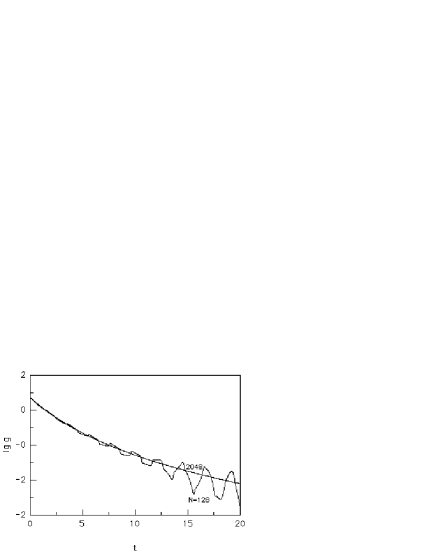
Figure 1: A decaying solution (6.2) at $x=0.6$ as a function of time. Obtained using MOL1(4) scheme and $cfl=1/2$. Solid lines - numerical solutions for $N=128$ and $N=2048$. The exact and $N=2048$ numerical solutions cannot be distinguished on this plot.

To understand this behavior of numerical schemes, it is instructive to consider a special case of exponential solutions (4.13) which can be investigated analytically. As an example, we take $\alpha=1$, $\beta=\gamma=0$ in (2.3). This choice of parameters gives a pair of exponential solutions (4.13) with the speed $a=\pm\frac{1}{\sqrt{2}}$,

$$g_{\pm}=\exp\left(x\pm\frac{t}{\sqrt{2}}\right).$$ (6.5)

We now attempt to obtain $g_{\pm}$ numerically on the interval $0\leq x\leq 1$ discretized using $N$ grid points,

$$x_{i}=\frac{1}{N}\left(i-\frac{1}{2}\right),\quad i=1,...,N,$$ (6.6)

and applying Robin boundary conditions ${\partial\ln g\over\partial{x}}=1$ for $i=0$ and $i=N+1$,

$$g_{0}=\exp(\ln g_{2}-2\Delta x\ln g_{1}),\quad g_{N+1}=\exp(\ln g_{N-1}+2\Delta x\ln g_{N}).$$ (6.7)

We use these boundary conditions because, in this particular case, they completely eliminate the influence of boundaries on a numerical solution in internal points (see below). For integration in time we use MOL1(4) with $cfl=\frac{1}{2}$. By varying Courant number in the range $1\leq cfl\leq\frac{1}{16}$ and Runge-Kutta order from $n=2$ to $n=4$ we verified that errors of integration in time in our numerical experiments are less than $10^{-4}$ of the truncation errors introduced by the spatial discretization (5.7).

Results of numerical integration for a decaying solution $g_{-}$ are shown in Figure 2 for resolutions $N=16$ through $N=1024$. In the beginning, numerical solutions follow the exact solution but eventually begin to deviate and grow exponentially. With increasing $N$, the exponential growth starts later. However, time $t_{s}$ of stable integration is proportional only to a logarithm of a number of grid points, $t_{s}\sim\ln N$. Integration beyond, say, $t\simeq 10$ would require an unpractical larger number $N>10^{6}$. Table 3 illustrates convergence of numerical solutions for two different moments of time, $t_{1}=1.2375$ and $t_{2}=3.7125$, which are both less than $t_{s}$. There is a second-order convergence at these times ( integration of $g_{+}$ does not present any difficulties and can be continued indefinitely).

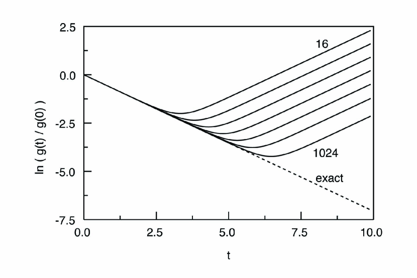
Figure 2: A decaying solution $g_{-}$ as a function of time. Obtained using a MOL1(4) integrator and $cfl=1/2$. Solid lines - numerical solutions with $N=16$ through $N=1024$. Dashed line - exact solution.

N $L_{\infty}(t1)$ $L_{\infty}(t2)$ 16 2.6421E-04 2.2272E-03 32 5.6685E-05 4.4543E-04 64 1.2938E-05 2.0090E-04 128 3.0747E-06 5.9922E-05 256 7.3409E-07 1.5723E-05

Table 3: Convergence of numerical solutions $g_{-}$ for two moments of time $t_{1}=1.2375$ and $t_{2}=3.7125$.

We now analyze the reason for an asymptotic instability discussed above. Using initial conditions $g_{i}(0)=exp(x_{i})$, we can present numerical solutions $g_{i}(t)$ at $t>0$ as

$$g_{i}(t)=f_{i}(t)\exp(x_{i}),\quad K_{i}(t)={\partial f_{i}\over\partial{t}}\exp(x_{i}),$$ (6.8)

where $f_{i}$ are functions of time. Substituting (6.8) into (5.7), we obtain a set of identical equations for all $f_{i}$,

$${\partial^{2}f_{i}\over\partial{t}^{2}}=cf_{i}-\frac{({\partial f_{i}\over\partial{t}})^{2}}{f_{i}}$$ (6.9)

where

$$c=\frac{e^{\Delta x}+e^{-\Delta x}-2}{\Delta x^{2}}=1+O(\Delta x^{2})\geq 1~{}$$ (6.10)

is a constant independent of $i$ (Robin boundary conditions (6.7) are necessary to ensure that (6.9) holds for the outermost grid points $i=1$ and $i=N$). Initial values $f_{i}(0)=1$ and ${\partial f_{i}(0)\over\partial{t}}=\pm\frac{1}{\sqrt{2}}$ are also identical for all $i$. We thus can ignore index $i$ in (6.9), and use a single ordinary differential equation

$${\partial^{2}f\over\partial{t}^{2}}=cf-\frac{({\partial f\over\partial{t}})^{2}}{f}$$ (6.11)

to describe numerical solutions $g_{i}(t)=f(t)\cdot g_{i}(0)$ at all grid points. Integration of (6.11) gives

$$\left({\partial f\over\partial{t}}\right)^{2}=\frac{cf^{2}}{2}+\frac{C}{f^{2}},$$ (6.12)

where $C=const$. We set it to $C=\frac{1-c}{2}\leq 0$ to satisfy initial conditions, and finally obtain the following differential equation

$$\frac{df}{dt}=\pm\sqrt{\frac{cf^{2}}{2}+\frac{1-c}{2f^{2}}}.$$ (6.13)

The value of $c=1$ corresponds to a continuum limit of $\Delta x\rightarrow 0$. Difference in the behavior of numerical and analytical solutions comes from the presence of the term $\frac{1-c}{2f^{2}}$. Note, that this term is $O(\Delta x^{2})$. Its variations do not change the second-order accuracy of the algorithm. The term is negative since $c>1$.

Consider first an exponentially growing solution $g_{+}$. For this solution, ${\partial f(0)\over\partial{t}}>0$. Therefore, we must initially take a $+$ sign in (6.13). The expression under the square root in (6.13) is positive at $t=0$ and it will only increase with increasing $f$ because the term $\frac{1-c}{2f^{2}}\rightarrow 0$ when $f\rightarrow\infty$. The relative difference between numerical and analytical solutions will tend to zero when $t\rightarrow\infty$ as well.

For a decaying solution $g_{-}$, asymptotic behavior of exact and numerical solutions is qualitatively different. For the exact solution, we have $K\rightarrow 0$ and $f\rightarrow 0$ when $t\rightarrow\infty$. But from (6.12) we observe that for $c$ other than zero $f$ cannot become zero because $\left({\partial f\over\partial{t}}\right)^{2}$ in (6.12) has a minimum ${\partial f\over\partial{t}}=0$ at a finite $f=f_{s}=(2(c-1)/c)^{1/4}>0$. For a decaying solution, ${\partial f(0)\over\partial{t}}<0$ and we must initially take $-$ sign in (6.13). When $f$ reaches the value of $f_{s}$ we have $df/dt=0$ but the second derivative remains positive

$$\frac{d^{2}f}{dt^{2}}=2cf+(c-1)/f^{3}>0.$$ (6.14)

As a result, the numerical solution switches at $f=f_{s}$ from $-$ branch to $+$ branch in (6.13), and begins to increase, $f\rightarrow\infty$ when $t\rightarrow\infty$.

We can estimate the moment of time, $t_{s}$, when the solution switches from the $-$ to the $+$ branch from

$$e^{-\frac{t_{s}}{\sqrt{2}}}\simeq f_{s}=(2(c-1)/c)^{1/4}\simeq\Delta x^{1/2}.$$ (6.15)

When the resolution is increased, $f_{s}$ becomes smaller and is reached at later time. But (6.15) shows that $t_{s}\propto(\ln\Delta x)^{-1}$. To increase a period of stable integration $t_{s}$ for a decaying solution, we must decrease $\Delta x$ (increase $N$) exponentially!

If we impose boundary conditions other than (6.7), deviations from the exact solution in internal points grow as described by (6.13) only until a signal from the boundary reaches them. After that, interaction with the boundary leads to a violent instability and a termination of numerical calculations. The reason for an instability observed for a decaying solution E2 (Figure 1) appears to be the same. Truncation errors lead to an imperfect balance of linear and non-linear terms, and to a deviation of a numerical solution from the exact one. Subsequent interaction with the boundaries amplifies these deviations, and the calculation eventually terminates.

7 Integration in logarithmic variables

We now show that logarithmic variables $\phi=\ln g$, $\psi=\phi_{t}$, and $\theta=\psi_{x}$ allow to significantly improve the accuracy and stability of numerical integration.

Equation (3.2) for $\phi$ can be integrated numerically using the same schemes CFLN1 and MOL1$(n)$. We must simply replace $g$, $K$ and $D$ in these schemes with $\phi$, $\psi$, and $\theta$, and to substitute the non-linear term $\cal R$ with its logarithmic counterpart $\cal S$ (3.6). The schemes than become

$${\rm CFLN1:}\quad\quad\left\{\begin{split}\quad&\bar{\psi}_{i}=\psi^{n-\frac{1}{2}}_{i}+\Delta t\left(\frac{\phi^{n}_{i+1}-2\phi^{n}_{i}+\phi^{n}_{i-1}}{\Delta x^{2}}+{\cal S}(\psi^{n-\frac{1}{2}}_{i},\theta_{i}^{n})\right)\quad(\rm predictor),\\ \quad&\psi_{i}^{n+\frac{1}{2}}=\bar{\psi}_{i}+\frac{\Delta t}{2}\left({\cal S}(\bar{\psi}_{i},\theta^{n}_{i})-{\cal S}(\psi^{n-\frac{1}{2}}_{i},\theta^{n}_{i})\right)\quad(\rm corrector),\\ \quad&\phi^{n+1}_{i}=\phi^{n}_{i}+\Delta t\,\psi^{n+\frac{1}{2}}_{i},\\ \end{split}\right.$$ (7.1)

and

$${\rm MOL1(n):}\quad\left\{\begin{split}\quad&{\partial\phi_{i}\over\partial{t}}=\psi_{i},\\ \quad&{\partial\psi_{i}\over\partial{t}}=\frac{\phi_{i+1}+\phi_{i-1}-2\phi_{i}}{\Delta x^{2}}+{\cal S}(\psi_{i},\theta_{i}),\end{split}\right.$$ (7.2)

where

$$\theta_{i}=\frac{\phi_{i+1}-\phi_{i-1}}{2\Delta x}$$ (7.3)

and

$${\cal S}_{i}=-(\alpha+1)\psi_{i}^{2}-(\beta-1)\theta_{i}^{2}-\gamma\psi_{i}\theta_{i}.$$ (7.4)

Schemes CFLN2 and MOL2 can be rewritten in a similar way.

Let us first consider how a CFLN1 scheme will reproduce an exponentially decaying solution $g_{-}$ (6.5). For this solution, initial conditions are $\phi^{0}_{i}=x_{i}$, a linear function of $x$, and $\psi^{-\frac{1}{2}}_{i}=\frac{1}{\sqrt{2}}$, a constant. With these conditions, the right-hand sides of the first two equations in (7.1) become zero, and it is easy to verify that $\psi_{i}$ remain constant through all subsequent time steps, whereas $\phi_{i}$ decrease with time linearly, $\phi^{n}_{i}=x_{i}-\frac{n\Delta t}{\sqrt{2}}$. The same is obviously true for MOL1. Transformed to logarithmic variables, CFLN1 and MOL1 reproduce exponential solutions exactly.

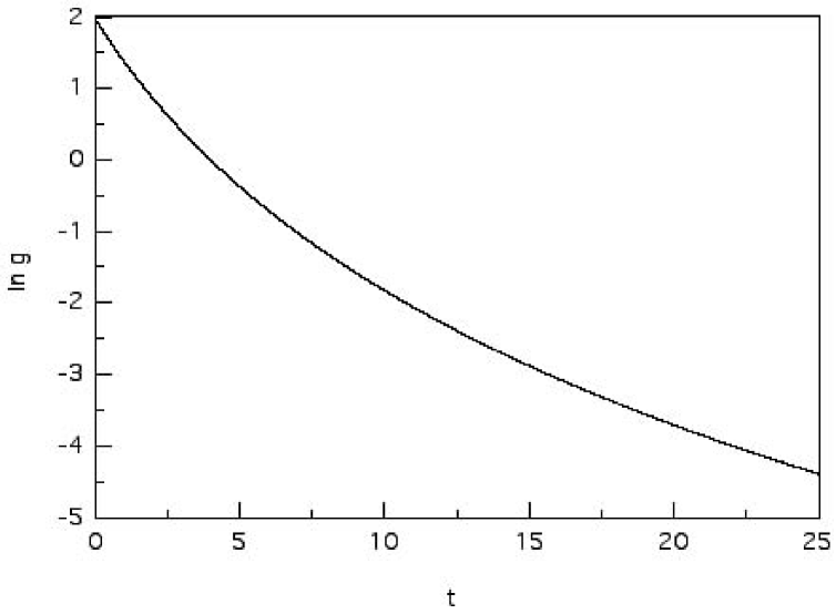
Figure 3: Decaying solutions (6.2) at $x=0.6$ as a function of time obtained in logarithmic variables using CFLN1 scheme with $cfl=1$. Solid lines - numerical solutions for $N=128$ and $N=2048$. Dashed line - exact solution. The solutions cannot be distinguished on the plot.

N $L_{\infty}(t1)$ CFLN1 $L_{\infty}(t2)$ CFLN1 $L_{\infty}(t1)$ MOL1 $L_{\infty}(t2)$ MOL1 32 3.9E-02 8.9E-02 4.1E-02 2.1E-01 64 1.3E-02 3.2E-02 1.3E-02 3.4E-02 128 3.4E-03 1.1E-02 3.7E-03 1.3E-02 256 8.7E-04 3.4E-03 9.1E-04 3.6E-03 512 2.1E-04 8.9E-04 2.1E-04 9.0E-04 1024 5.2E-05 2.2E-04 5.2E-05 2.2E-04

Table 4: Convergence of numerical solutions (6.2) for two moments of time $t_{1}=20$ and $t_{2}=50$ using logarithmic variables and two numerical schemes, CFLN1 with CFL number $cfl=1$ and MOL1(4) with $cfl=0.5$. The error norm $L_{\infty}={\rm max}_{i}|g_{i}/g_{e}-1|$, where $g_{e}$ is the exact solution.

Next, we test the reformulated schemes on a decaying solution (6.2). Figure 3 shows numerical solutions at $x=0.6$ as a function of $t$ obtained using CFL1 scheme, and it must be compared to Figure 1. Table 4 illustrates convergence of reformulated CFLN1 and MOL1 schemes with increasing $N$ and should be compared with Table 2. We see from the comparison that logarithmic variables greatly reduce errors of numerical integration.

8 Conclusions

In this paper we introduced a scalar wave equation with non-linear terms similar to those of more complex equations of general relativity. The equation has a number of non-trivial analytical solutions useful for testing numerical schemes.

We formulated two classes of finite-difference schemes for numerical integration of this equation. One (CFLN) is a non-linear extension of a classical second-order central difference scheme for a linear scalar wave equation [3]. Another (MOL) is based on a method-of-lines approach. The schemes have a comparable accuracy but MOL requires a larger number of right-hand side evaluations.

Both schemes converge to exact solutions at any fixed $t$ when numerical resolution is increased, $\Delta x\rightarrow 0$. For some of the solutions, however, integration becomes unstable when resolution is kept fixed and $t$ is increased. We trace this behavior to deviations from a perfect balance between linear and non-linear terms caused by discretization. As a result, the asymptotic behavior of numerical solutions may differ qualitatively from the asymptotic behavior of the corresponding exact solutions of a partial differential equation. An important point is that these deviations happen without violating a second-order accuracy. Therefore, having both convergence at finite $t$ and an asymptotic instability is not a contradiction.

An asymptotic instability seems not to be a fault of a particular numerical scheme. All schemes tested in this paper display this phenomenon regardless of how numerical solutions are advanced in time. CFLN, Runge-Kutta, and ICN-type integration results in the same asymptotic instability. We have no reason to believe that this phenomenon should be limited only to scalar non-linear equations. Examples presented in the paper clearly demonstrate that second-order accuracy of spatial discretization, although necessary for obtaining convergent numerical solutions at finite $t$, is not a guarantee of a correct asymptotic behavior of a numerical scheme.

Finally, we have shown that an exponential transformation (3.1) leads to a significant improvement in accuracy and stability of numerical algorithms. We do not know if some of the difficulties encountered in numerical general relativity steam from a similar non-linear asymptotic instability, and whether integration of GR equations can be improved by an exponential transformation of variables. We believe that these questions are worth investigating. In the accompanying paper we show how an exponential transformation of variables can be carried out for tensorial equations of GR. Numerical schemes formulated in this paper can be extended to GR equations written in both second-order (CFLN1 and MOL1) and first-order forms (CFLN2 and MOL2).

This work was supported in part by the NASA grant SPA-00-067, Danish Natural Science Research Council through grant No 94016535, Danmarks Grundforskningsfond through its support for establishment of the Theoretical Astrophysics Center, and by the Naval Research Laboratory through the Office of Naval Research. We thank Kip Thorne, Jacob Hansen, and Ryoji Takahashi for useful discussions. I.D. thanks the Naval Research Laboratory, A.K. thanks the Theoretical Astrophysics Center, and both authors thank Caltech for hospitality during their visits.

References

- [1] Hisa aki Shinkai and Gen Yoneda. Re-formulating the Einstein equations for stable numerical simulations, 2002, gr-qc/0209111.
- [2] A.M. Khokhlov and I.D. Novikov. Gauge stability of 3 + 1 formulations of general relativity. Class. Quantum Grav., 19:827–846, 2002.
- [3] R. Courant, K.O. Friedrichs, and H. Lewy. Math. Ann., 100:32, 1928.
- [4] R.D. Richtmyer and K.W. Morton. Difference methods for initial-value problems. John Wiley and Sons, New York, 1967.
- [5] J. Hansen, A.M. Khokhlov and I.D. Novikov, in preparation.
- [6] S. A. Teukolsky. Stability of the iterated Crank-Nicholson method in numerical relativity. Phys. Rev., D61:087501, 2000.