Effective Gravitational Equations on Brane World with Induced Gravity

Abstract

We present the effective equations to describe the four-dimensional gravity of a brane world, assuming that a five-dimensional bulk spacetime satisfies the Einstein equations and gravity is confined on the $Z_{2}$ symmetric brane. Applying this formalism, we study the induced-gravity brane model first proposed by Dvali, Gabadadze and Porrati. In a generalization of their model, we show that an effective cosmological constant on the brane can be extremely reduced in contrast to the case of the Randall-Sundrum model even if a bulk cosmological constant and a brane tension are not fine-tuned.

]

I Introduction

There has been tremendous interest over the last several years in this brane world scenario. String theory predicts a boundary layer, a brane, on which edges of open strings stand[1]. The existence of such natural boundaries suggests a new perspective in cosmology; a brane world scenario, that is, we are living in a three-dimensional (3-D) hypersurface in a higher-dimensional spacetime[2]. In contrast to the original Kaluza-Klein picture in which we live in four-dimensional (4-D) spacetime with extra compactified “internal space”, our world view appears to be changed completely. Particles in the standard model are expected to be confined to the brane, whereas the gravitons propagate in the entire bulk spacetime. This gives an interesting feature in the brane world, because TeV gravity might be realistic and a quantum gravity effect could be observed by a next-generation particle collider[3]. Randall and Sundrum (RS) also proposed two new mechanisms [4]: one may provide us with a resolution of the hierarchy problem by a small extra dimension, and the other is an alternative compactification of extra dimensions. In the second model, they showed that 4-D Newtonian gravity is recovered at low energies, because gravity is confined in a single positive-tension brane even if the extra dimension is not compact.

If the brane world is real, one may find some evidences of higher-dimensions in strong gravity phenomena. Here we shall study some classes of the brane models, in which gravity is confined on the brane as the Randall-Sundrum second model. Assuming that a spacetime is five-dimensional(5-D), we first derive the effective “Einstein equations” for the 4-D brane metric obtained by projecting the 5-D metric onto the brane world[5, 6, 7, 8]. The gravitational action on the brane, which may be induced via quantum effects of matter fields, could be arbitrary in the present approach. This approach yields the most general form of the 4-D gravitational field equations for a brane world observer whatever the form of the bulk metric, in contrast to the usual Kaluza-Klein type dimensional reduction which relies on taking a particular form for the bulk metric in order to integrate over the extra dimensions. The price to be paid for such generality, is that the brane world observer may be subject to influences from the bulk, which are not constrained by local quantities, i.e., the set of 4-D equations does not in general form a closed system. Nonetheless, when the brane is located at an orbifold fixed point under $Z_{2}$ symmetry the energy-momentum tensor on the brane is sufficient to determine the extrinsic curvature of the brane, and together with the local induced metric, this strongly constrains the brane world gravity. In particular, a Friedmann equation for an isotropic and homogeneous brane universe is completely determined up to an integration constant. As a concrete example, we apply our formalism to the induced gravity brane model proposed by Dvali, Gabadadze and Porrati[9], and show how we obtain the accelerating universe at low energy scale without a cosmological constant (or a quintessential potential). For this model, many authors discussed the geometrical aspects [10, 11, 12, 13, 14] as well as cosmology [15, 16, 17]. Generalizing their model to the case with a bulk cosmological constant and a tension of the brane and assuming the energy scale of the tension is much larger than the 5-D Planck mass, we show that the effective cosmological constant on the brane is extremely reduced in contrast to the RS model even if the cosmological constant and the tension are not fine-tuned.

II The effective gravitational equations in a brane scenario

We consider a 5-D bulk spacetime with a single 4-D brane, on which gravity is confined, and derive the effective 4-D gravitational equations.

Suppose that the 4-D brane $(M,g_{\mu\nu})$ is located at a hypersurface (${\cal B}(X^{A})=0$) in the 5-D bulk spacetime $({\cal M},{}^{(5)}g_{AB})$, of which coordinates are described by $X^{A}~{}(A=0,1,2,3,5)$. We assume the most generic action for the brane world, although the simple Einstein-Hilbert action is adopted in the 5-D spacetime. The action discussed here is then

$$S=S_{\rm bulk}+S_{\rm brane},$$ (1)

where

$$S_{\rm bulk}=\int_{\cal M}d^{5}X\sqrt{-{}^{(5)}g}\left[{1\over 2\kappa_{5}^{2}}{}^{(5)}R+{}^{(5)}L_{\rm m}\right],$$ (2)

and

$$S_{\rm brane}=\int_{M}d^{4}x\sqrt{-g}\left[{1\over\kappa_{5}^{2}}K^{\pm}+L_{\rm brane}(g_{\alpha\beta},\psi)\right].$$ (3)

$\kappa_{5}^{2}$ is the 5-D gravitational constant, ${}^{(5)}R$ and ${}^{(5)}L_{\rm m}$ are the 5-D scalar curvature and the matter Lagrangian in the bulk, respectively. $x^{\mu}~{}(\mu=0,1,2,3)$ are the induced 4-D coordinates on the brane, $K^{\pm}$ is the trace of extrinsic curvature on either side of the brane[18, 19] and $L_{\rm brane}(g_{\alpha\beta},\psi)$ is the effective 4-D Lagrangian, which is given by a generic functional of the brane metric $g_{\alpha\beta}$ and matter fields $\psi$.

The 5-D Einstein equations in the bulk are

$${}^{(5)}G_{AB}=\kappa_{5}^{2}\,\,\left[\,{}^{(5)}T_{AB}+\tau_{AB}\,\delta({\cal B})\,\right]\,,$$ (4)

where

$${}^{(5)}T_{AB} \equiv -2{\delta{}^{(5)}\!L_{\rm m}\over\delta{}^{(5)}g^{AB}}+{}^{(5)}g_{AB}{}^{(5)}\!L_{\rm m}\,$$ (5)

is the energy-momentum tensor of bulk matter fields, while $\tau_{\mu\nu}$ is the “effective” energy-momentum tensor localized on the brane which is defined by

$$\tau_{\mu\nu}\equiv-2{\delta L_{\rm brane}\over\delta g^{\mu\nu}}+g_{\mu\nu}L_{\rm brane}\,.$$ (6)

The $\delta({\cal B})$ denotes the localization of brane contributions. We would stress that $\tau_{\mu\nu}$ usually contains curvature contributions from induced gravity. In that term, we can also include “non-local” contributions such as a trace anomaly[20, 21], although those contributions are not directly derived from the effective Lagrangian $L_{\rm brane}$.

The basic equations in the brane world are obtained by projection of the variables onto the brane world, because we assume that the gravity on the brane is confined. The induced 4-D metric is $g_{AB}={}^{(5)}g_{AB}-n_{A}n_{B},$ where $n_{A}$ is the spacelike unit-vector field normal to the brane hypersurface $M$.

Following Ref. [5], in which we have just to replace ordinary energy-momentum tensor $\tau_{\mu\nu}$ with new one[8, 11], we obtain the gravitational equations on the brane world as

$$G_{\mu\nu} = {2\kappa_{5}^{2}\over 3}\biggl{[}{}^{(5)}T_{RS}~{}g^{R}_{~{}\mu}g^{S}_{~{}\nu}+g_{\mu\nu}\biggl{(}{}^{(5)}T_{RS}~{}n^{R}n^{S}$$ (8)

$$~{}~{}~{}~{}~{}~{}~{}~{}-{1\over 4}{}^{(5)}T\biggr{)}\biggr{]}+\kappa_{5}^{4}\pi_{\mu\nu}-E_{\mu\nu}\,,$$

$$D_{\nu}\tau^{~{}\nu}_{\mu}=-2\,{}^{(5)}T_{RS}\,n^{R}g^{S}_{~{}\mu},$$ (9)

where

$$\pi_{\mu\nu}=-\frac{1}{4}\tau_{\mu\alpha}\tau_{\nu}^{~{}\alpha}+\frac{1}{12}\tau\tau_{\mu\nu}+\frac{1}{8}g_{\mu\nu}\tau_{\alpha\beta}\tau^{\alpha\beta}-\frac{1}{24}g_{\mu\nu}\tau^{2}\,$$ (10)

and

$$E_{\mu\nu}={}^{(5)}C_{MRNS}~{}n^{M}n^{N}g_{~{}\mu}^{R}~{}g_{~{}\nu}^{S}.$$ (11)

Eqs. (8)-(10) give the effective gravity theory on the brane. These are formally the same as those in Ref.[5]. In fact, if the brane Lagrangian $L_{\rm brane}$ contains only matter fields $\psi$, $\tau_{\mu\nu}$ is just the energy-momentum tensor of the matter fields, and then the gravity is described by the 4-D Einstein tensor in Eq. (8)[5]. Then we recover the Einstein gravitational theory in the 4-D brane world. If $L_{\rm brane}$ includes, however, some additional contributions of gravity such as an induced gravity on the brane, the effective energy-momentum tensor $\tau_{\mu\nu}$ gives modification of gravitational interaction in the effective theory.

III Dvali-Gabadadze-Porrati’s type Models

We study the case with an induced gravity on the brane due to quantum corrections. If we take into account quantum effects of matter fields confined on the brane, the gravitational action on the brane will be modified. Here we shall discuss a brane world model proposed by Dvali, Gabadadze, and Porrati[9]. The interaction between bulk gravity and the matter on the brane induces gravity on the brane through its quantum effect. Their model based on this brane-induced gravity could be interesting because, phenomenologically, 4-D Newtonian gravity on a brane world is recovered at high energy scale, whereas 5-D gravity emerges at low energy scale.

We then consider the brane Lagrangian

$$L_{\rm brane}={\mu^{2}\over 2}R-\lambda+L_{\rm m}\,,$$ (12)

where $\mu$ is a mass scale which may correspond to the 4-D Planck mass. We also assume that the 5-D bulk space includes only a cosmological constant ${}^{(5)}\Lambda$. It is just a generalized version of the Dvali-Gabadadze-Porrati model, which is obtained by setting $\lambda=0$ as well as ${}^{(5)}\Lambda=0$ (see also the discussion by Tanaka[22]).

A Effective Gravitational Equations

In order to find the basic equations on the brane, we just calculate the “energy-momentum” tensor of the brane $\tau_{\mu\nu}$ by the definition (6) from the Lagrangian (12)

$$\tau^{\mu}_{~{}\nu}=-\lambda\delta^{\mu}_{~{}\nu}+T^{\mu}_{~{}\nu}-\mu^{2}G^{\mu}_{~{}\nu}.$$ (13)

Inserting this equation into Eq. (8), we find the effective equations for 4-D metric $g_{\mu\nu}$ as

$$\left(1+{\lambda\over 6}\kappa_{5}^{4}\mu^{2}\right)G_{\mu\nu}+\kappa_{5}^{4}\mu^{2}{\cal K}_{\mu\nu\rho\sigma}(T_{\alpha\beta})G^{\rho\sigma}+\Lambda g_{\mu\nu}$$ (14)

$$~{}~{}~{}~{}~{}~{}~{}~{}~{}~{}={\lambda\over 6}\kappa_{5}^{4}T_{\mu\nu}+\kappa_{5}^{4}\left[\pi_{\mu\nu}^{(T)}+\mu^{4}\pi^{(G)}_{\mu\nu}\right]-E_{\mu\nu},$$ (15)

where

$${\cal K}_{\mu\nu\rho\sigma} = {1\over 4}\left(g_{\mu\nu}T_{\rho\sigma}-g_{\mu\rho}T_{\nu\sigma}-g_{\nu\sigma}T_{\mu\rho}\right)$$ (17)

$$~{}~{}+{1\over 12}\Bigl{[}T_{\mu\nu}g_{\rho\sigma}+T\left(g_{\mu\rho}g_{\nu\sigma}-g_{\mu\nu}g_{\rho\sigma}\right)\Bigr{]},\,$$

$$\Lambda = {1\over 2}\left[{}^{(5)}\Lambda+{1\over 6}\kappa_{5}^{4}\lambda^{2}\right],$$ (18)

$$\pi_{\mu\nu}^{(T)} = -\frac{1}{4}T_{\mu\alpha}T_{\nu}^{~{}\alpha}+\frac{1}{12}TT_{\mu\nu}$$ (20)

$$~{}~{}+\frac{1}{8}g_{\mu\nu}T_{\alpha\beta}T^{\alpha\beta}-\frac{1}{24}g_{\mu\nu}T^{2},$$

$$\pi_{\mu\nu}^{(G)} = -\frac{1}{4}G_{\mu\alpha}G_{\nu}^{~{}\alpha}+\frac{1}{12}GG_{\mu\nu}$$ (22)

$$~{}~{}+\frac{1}{8}g_{\mu\nu}G_{\alpha\beta}G^{\alpha\beta}-\frac{1}{24}g_{\mu\nu}G^{2}.$$

The Codazzi equation is now $D^{\nu}\tau_{\mu\nu}=0$, which implies the energy momentum conservation, i.e.

$$D^{\nu}T_{\mu\nu}=0\,,$$ (23)

because of the Bianchi identity.

First we discuss the vacuum case, $T_{\mu\nu}=0$. Assuming $\Lambda=0$ and $E_{\mu\nu}=0$, we find

$$\left(1+{\lambda\over 6}\kappa_{5}^{4}\mu^{2}\right)G_{\mu\nu}=\kappa_{5}^{4}\mu^{4}\pi^{(G)}_{\mu\nu}\,.$$ (24)

If the spacetime is a maximally symmetric, setting $R_{\mu\nu}={1\over 4}Rg_{\mu\nu}$ ($R\neq 0$), we obtain

$$R={8\rho_{0}\over\mu^{2}}\,,$$ (25)

where

$$\rho_{0}=m_{\lambda}^{4}+6{m_{5}^{6}\over\mu^{2}}\,,$$ (26)

with two mass scales; $m_{\lambda}=\lambda^{1/4}$ and $m_{5}=\kappa_{5}^{-2/3}$. Introducing the scale length $L_{DS}=\sqrt{12/R}$, we find

$$H_{DS}\equiv L_{DS}^{-1}={1\over\mu}\sqrt{2\rho_{0}\over 3}\,.$$ (27)

This $H_{DS}$ gives the Hubble parameter of late time inflation without a cosmological constant, which was shown by Dvali et al in the case of $m_{\lambda}=0$ and ${}^{(5)}\Lambda=0$, i.e. $H_{DS}=2m_{5}^{3}/\mu^{2}$ or equivalently $\Lambda_{\rm eff}=12m_{5}^{6}/\mu^{4}$[9].

B Friedmann-Robertson-Walker universe

Now we discuss the Friedmann-Robertson-Walker universe with a perfect fluid. Since the spacetime is isotropic and homogeneous, we can show $D^{\nu}\pi_{\mu\nu}=0$ following [5], which implies

$$D^{\nu}E_{\mu\nu}=0.$$ (28)

The basic equations (8) are

$$G^{0}_{~{}0} = -{1\over 2}{}^{(5)}\!\Lambda+\kappa_{5}^{4}\pi^{0}_{~{}0}-E^{0}_{~{}0},$$ (29)

$$G^{i}_{~{}j} = -{1\over 2}{}^{(5)}\!\Lambda\delta^{i}_{~{}j}+\kappa_{5}^{4}\pi^{i}_{~{}j}-E^{i}_{~{}j},$$ (30)

where

$$G^{0}_{~{}0} = -3\left(H^{2}+{k\over a^{2}}\right),$$ (31)

$$G^{i}_{~{}j} = -\left(2\dot{H}+3H^{2}+{k\over a^{2}}\right)\delta^{i}_{~{}j},$$ (32)

and

$$\pi^{0}_{~{}0} = -{1\over 12}\left(\tau^{0}_{~{}0}\right)^{2},$$ (33)

$$\pi^{i}_{~{}j} = {1\over 12}\tau^{0}_{~{}0}\left(\tau^{0}_{~{}0}-2\tau^{1}_{~{}1}\right)\delta^{i}_{~{}j},$$ (34)

with

$$\tau^{0}_{~{}0} = -(\lambda+\rho)-\mu^{2}G^{0}_{~{}0},$$ (35)

$$\tau^{i}_{~{}j} = (P-\lambda)\delta^{i}_{~{}j}-\mu^{2}G^{i}_{~{}j}.$$ (36)

Eqs. (29) and (30) are written as

$$3X={1\over 2}{}^{(5)}\Lambda+E^{0}_{~{}0}+{\kappa_{5}^{4}\over 12}\left(\lambda+\rho-3\mu^{2}X\right)^{2},$$ (37)

$$\left[1+{\kappa_{5}^{4}\over 6}\mu^{2}\left(\lambda+\rho-3\mu^{2}X\right)\right]Y$$ (38)

$$~{}~{}~{}~{}~{}~{}=-{2\over 3}E^{0}_{~{}0}-{\kappa_{5}^{4}\over 12}(\rho+P)\left(\lambda+\rho-3\mu^{2}X\right),$$ (39)

where

$$X = H^{2}+{k\over a^{2}},$$ (40)

$$Y = \dot{H}-{k\over a^{2}}.$$ (41)

From Eq. (28), we find the equation for $E^{0}_{~{}0}$ as

$$\dot{E}^{0}_{~{}0}+4HE^{0}_{~{}0}=0.$$ (42)

This equation, which is the same as the dark radiation in the case of the RS model[5], is easily integrated as

$$E^{0}_{~{}0}={{\cal E}_{0}\over a^{4}},$$ (43)

where ${\cal E}_{0}$ is just an integration constant.

We now have to solve one equation (37), which is a quadratic equation with respect to $X$ and then rewritten as

$$H^{2}+{k\over a^{2}}={1\over 3\mu^{2}}\Bigl{[}\,\rho+\rho_{0}\bigl{(}1+\epsilon{\cal A}(\rho,a)\bigr{)}\,\Bigr{]}\,,$$ (44)

where $\epsilon$ denotes either $+1$ or $-1$. ${\cal A}$ is defined by

$${\cal A} \equiv \left[{\cal A}_{0}^{2}+{2\eta\over\rho_{0}}\left(\rho-\mu^{2}{{\cal E}_{0}\over a^{4}}\right)\right]^{1\over 2},$$ (45)

where

$${\cal A}_{0} = \sqrt{1-2\eta{\mu^{2}\Lambda\over\rho_{0}}},$$ (46)

$$\eta = {6m_{5}^{6}\over\rho_{0}\mu^{2}}~{}~{}~{}(0<\eta\leq 1)\,.$$ (47)

This is just the Friedmann equation of our model. Since ${\cal A}$ does not vanish in generic situation, the sign of $\epsilon$ is determined by the initial condition of the universe. The choice of the sign of $\epsilon$ also has a geometrical meaning as shown by Deffayet, who analized the present model by embedding a brane in the 5-D bulk spacetime[15].

C Effective Friedmann equations

To understand the behaviors of the Dvali et al’s cosmological model, we rewrite the basic equation (44) in the form of the conventional Friedmann equation as

$$H^{2}+{k\over a^{2}}={1\over 3}\Lambda_{\rm eff}^{(\epsilon)}+{8\pi G_{\rm eff}^{(\epsilon)}\over 3}\left(\rho+\rho_{\rm DR}^{(\epsilon)}\right),$$ (48)

where

$$\Lambda_{\rm eff}^{(\epsilon)} = {\rho_{0}\over\mu^{2}}\left(1+\epsilon{\cal A}_{0}\right),$$ (49)

$$8\pi G_{\rm eff}^{(\epsilon)} = {1\over\mu^{2}}\left[1+\epsilon{\cal F}(\rho,a)\right],$$ (50)

$$8\pi G_{\rm eff}^{(\epsilon)}\rho_{\rm DR}^{(\epsilon)} = -\epsilon{\cal F}(\rho,a){{\cal E}_{0}\over a^{4}},$$ (51)

with

$${\cal F}(\rho,a)={2\eta\over{\cal A}_{0}+{\cal A}(\rho,a)}\,.$$ (52)

Using the above expression, we may discuss the evolution of the universe. $\Lambda_{\rm eff}^{(\epsilon)}$ acts as a cosmological constant in each branch. The effective gravitational “constant” $G_{\rm eff}^{(\epsilon)}$ and the energy density of “dark energy” $\rho_{\rm DR}^{(\epsilon)}$ change in the history of the universe. To show them explicitly, we first give the asymptotic behaviors of ${\cal A}(\rho,a)$ and ${\cal F}(\rho,a)$, which are easily obtained as

$${\cal A}(\rho,a) \rightarrow \sqrt{{2\eta\over\rho_{0}}\left(\rho-\mu^{2}{{\cal E}_{0}\over a^{4}}\right)}\rightarrow\infty,$$ (53)

$${\cal F}(\rho,a) \rightarrow ~{}~{}~{}~{}~{}~{}{2\eta\over{\cal A}(\rho,a)}~{}~{}~{}~{}~{}~{}\rightarrow 0,$$ (55)

$$~{}~{}~{}{\rm as}~{}~{}\rho\rightarrow\infty~{}{\rm and}~{}a\rightarrow 0,$$

and

$${\cal A}(\rho,a)\rightarrow {\cal A}_{0},~{}~{}~{}~{}~{}{\cal F}(\rho,a)\rightarrow{\eta\over{\cal A}_{0}},$$ (57)

$$~{}~{}~{}{\rm as}~{}~{}\rho\rightarrow 0~{}{\rm and}~{}a\rightarrow\infty,$$

We then obtain the evolution of $G_{\rm eff}^{(\epsilon)}$ as follows:
As $\rho$ decreases from $\infty$ to zero (and $a$ increases from 0 to $\infty$), $8\pi G_{\rm eff}^{(\epsilon)}$ changes as

$$8\pi G_{\rm eff}^{(\epsilon)}~{}:~{}{1\over\mu^{2}}~{}\rightarrow~{}{1\over\mu^{2}}\left(1+{\epsilon\eta\over{\cal A}_{0}}\right).$$ (58)

The “effective” gravitational constant changes in time. In particular, in the negative branch ($\epsilon=-1$), if $\eta>\eta_{\rm cr}$, where

$$\eta_{\rm cr}\equiv-\mu^{2}{\Lambda\over\rho_{0}}+\sqrt{1+\left(\mu^{2}{\Lambda\over\rho_{0}}\right)^{2}}\,,$$ (59)

$G_{\rm eff}^{(-)}$ vanishes at some density and becomes negative below that density. In this case, $\eta\leq 1$ implies $\eta_{\rm cr}<1$, which requires $\Lambda>0$.

The expansion of the universe first slows down after this critical point, and then approaches some constant given by $\Lambda_{\rm eff}^{(-)}(>0)$. This cosmological model could be interesting because the expansion gets slow in some period of the universe and then it might help structure formation process. Note that although the effective gravitational constant in the Friedmann equation becomes negative now, it does not naively mean the Newtonian gravitational constant is negative. We need further analysis to check it.

As for $\rho_{\rm DR}^{(\epsilon)}$, we naively obtain that

$$8\pi G_{\rm eff}^{(\epsilon)}\rho_{\rm DR}^{(\epsilon)}~{}:~{}0~{}\rightarrow~{}{\cal C}^{(\epsilon)}{{\cal E}_{0}\over a^{4}},$$ (60)

where ${\cal C}^{(\epsilon)}=-\epsilon\eta/{\cal A}_{0}$. We need, however, further analysis in the high-density limit (and in the limit of $a=0$) (see Sec. III D).

Eq. (39) is also rewritten as

$$\dot{H}-{k\over a^{2}} = -{1\over 2\mu^{2}}\left(P+\rho\right)\left[1+{\epsilon\eta\over{\cal A}(\rho,a)}\right]+{2\epsilon\eta\over 3{\cal A}(\rho,a)}{{\cal E}_{0}\over a^{4}}.$$ (61)

Assuming the equation of state of the matter fluid is given by the adiabatic index $\gamma$ as

$$P=(\gamma-1)\rho\,,$$ (63)

and writing Eq. (LABEL:Friedmann2) in the conventional form as

$$\dot{H}-{k\over a^{2}} = -4\pi G_{\rm eff}^{(\epsilon)}\left(\gamma_{\rm eff}^{(\epsilon)}\rho+\gamma_{\rm DR}\rho_{\rm DR}^{(\epsilon)}\right),$$ (64)

where

$$\gamma_{\rm eff}^{(\epsilon)} = \gamma\left[1-{\epsilon\eta(\rho-\mu^{2}{\cal E}_{0}/a^{4}){\cal F}(\rho,a)\over\rho_{0}{\cal A}(\rho,a)[{\cal A}(\rho,a)+{\cal A}_{0}+2\epsilon\eta]}\right],$$ (65)

$$\gamma_{\rm DR} = {2\over 3}\left[1+{{\cal A}_{0}\over{\cal A}(\rho,a)}\right]\,,$$ (66)

we can define the effective adiabatic index of matter fluid ($\gamma_{\rm eff}^{(\epsilon)}$) and that of dark radiation ($\gamma_{\rm DR}$). Remind that the right-hand side of the conventional Friedmann equation with the above equation of state (63) is given by $-4\pi G\gamma\rho$.

We easily find the behavior of the effective adiabatic indexes $\gamma_{\rm eff}^{(\epsilon)}$ when $\rho$ (or $1/a$) changes from $\infty$ to 0 as follows:
For the positive branch ($\epsilon=+1$),

$$\gamma_{\rm eff}^{(+)}:\gamma~{}\searrow~{}\gamma_{\rm min}(\eta)~{}\nearrow~{}\gamma~{},$$ (67)

(see Fig 1(a)). This behavior is interesting because the “effective” negative pressure ($\gamma_{\rm eff}^{(+)}<1$) can be obtained during the evolution of the universe from standard matter fluid such as dust ($\gamma=1$).

As for the negative branch ($\epsilon=-1$), it is a little complicated (see Fig 1(b)). If $\eta<\eta_{\rm cr}$, as $\rho$ (or $1/a$) decreases from $\infty$ to 0,

$$\gamma_{\rm eff}^{(-)}:\gamma~{}\nearrow~{}\gamma_{\rm max}(\eta)~{}\searrow~{}\gamma\,,$$ (68)

while, for $\eta=\eta_{\rm cr}$ (which requires $\Lambda\geq 0$),

$$\gamma~{}~{}~{}~{}~{}~{}~{}~{}~{}\nearrow~{}~{}~{}~{}~{}~{}~{}~{}2\gamma\,.$$ (69)

If $\eta>\eta_{\rm cr}$ (which requires $\Lambda>0$),

$$\gamma_{\rm eff}^{(-)}: \gamma~{}\nearrow~{}+\infty,~{}-\infty~{}\nearrow~{}\gamma.$$ (70)

Here $\gamma_{\rm min}$ and $\gamma_{\rm max}$ depend on $\eta$, but $2\gamma\geq\gamma_{\rm max}>\gamma>\gamma_{\rm min}\geq\gamma/2\geq 0$. $\gamma_{\rm min}=\gamma/2$ is found when ${\cal A}_{0}=0$, while $\gamma_{\rm max}=2\gamma$ is obtained in the limit of $\eta=\eta_{\rm cr}$.

In Eq. (70), although $\gamma_{\rm eff}^{(-)}$ diverges at some density, Eq. (64) is not singular because $G_{\rm eff}^{(-)}$ vanishes at the same density. When $\gamma_{\rm eff}^{(-)}$ vanishes, which always occurs below that density, $H$ reaches a minimum value (if there is no dark radiation and $k=0$), and then it increases to some constant as we discussed above.

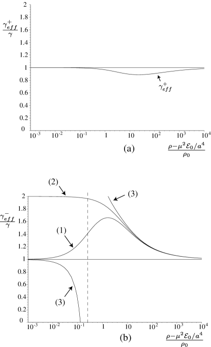
FIG. 1.: The schematic behavior of $\gamma_{\rm eff}^{(\pm)}$. On the top ((a)), we show one typical example for positive branch ($\epsilon=+1$) , while, on the bottom ((b)), we depict the figures for negative branch ($\epsilon=-1$) in the following three typical cases; (1) $\eta<\eta_{cr}$, (2) $\eta=\eta_{cr}$ and (3) $\eta>\eta_{cr}$. For an expanding universe, the universe evolves from the right hand side to the left in the figures.

As for dark radiation, the adiabatic index $\gamma_{\rm DR}$ does not depend on the branch and changes from 2/3 to 4/3 when $\rho$ changes as $\infty\rightarrow 0$. This means that in the early stage of the universe, the dark radiation does not behave as “radiation” but as “curvature” term (see below).

Next we discuss the dynamics of the universe in each limit separately.

D high density limit

In high density limit, we assume that $a\rightarrow 0$ as well as $\rho\gg\rho_{0}$. In this limit, we find

$$8\pi G_{\rm eff}^{(\epsilon)}\rho \approx {1\over\mu^{2}}\left(1+\epsilon{2\eta\over{\cal A}}\right)\rho,$$ (71)

$$8\pi G_{\rm eff}^{(\epsilon)}\rho_{\rm DR}^{(\epsilon)} \approx -\epsilon{2\eta\over{\cal A}}{{\cal E}_{0}\over a^{4}}\,,$$ (72)

and then we obtain from Eq. (48)

$$H^{2}+{k\over a^{2}}\approx{1\over 3\mu^{2}}\left[\rho+\epsilon\rho_{0}\sqrt{{2\eta\over\rho_{0}}\left(\rho-\mu^{2}{{\cal E}_{0}\over a^{4}}\right)}\right].$$ (73)

From the energy-momentum conservation of a perfect fluid, we have $\rho\propto a^{-3\gamma}$. We then classify the behavior of the early universe into three cases:
(1) $\gamma\geq 4/3$
This universe is the same as that in the conventional Einstein gravity, i.e. $a\propto t^{2/3\gamma}$.
(2) $2/3<\gamma<4/3$
Since the dark radiation term inside of the square root in Eq. (73) becomes dominant in the limit of $a\rightarrow 0$, ${\cal E}_{0}\leq 0$ is required. However the linear density term dominates the dark radiation. As a result, we again find the same expansion law as that in the conventional Einstein gravity ($a\propto t^{2/3\gamma}$). If ${\cal E}_{0}>0$, we may find a singularity at a finite scale factor.
(3) $0\leq\gamma\leq 2/3$
In this case, ${\cal E}_{0}<0$ is required, otherwise the universe evolves into a singularity with a finite value of scale factor. If ${\cal E}_{0}<0$ the dark radiation term gives the largest contribution on the right hand side of Eq. (73), which is the similar to the curvature term. Then we find that Eq. (73) is reduced to

$$H^{2}+{\tilde{k}\over a^{2}}\approx{\rho\over 3\mu^{2}}\,,$$ (74)

where

$$\tilde{k}=k-\epsilon{2m_{5}^{3}\over\sqrt{3}\mu^{2}}\sqrt{|{\cal E}_{0}|}\,.$$ (75)

This gives the conventional inflationary solution. For $\gamma=0$, setting $\tilde{H}_{0}=\sqrt{\rho/(3\mu^{2})}$, we find exponential expansion

$$a=\left\{\begin{array}[]{c}{\sqrt{\tilde{k}}\over\tilde{H}_{0}}\cosh[\tilde{H}_{0}t]~{}~{}~{}~{}({\rm for}~{}~{}\tilde{k}>0)\\[5.0pt] a_{0}\exp[\tilde{H}_{0}t]~{}~{}~{}~{}({\rm for}~{}~{}\tilde{k}=0)\\[5.0pt] {\sqrt{|\tilde{k}|}\over\tilde{H}_{0}}\sinh[\tilde{H}_{0}t]~{}~{}~{}~{}({\rm for}~{}~{}\tilde{k}<0)\end{array}~{}\right.$$ (79)

We then obtain non-singular universe even for $k=-1$ in the case of $\epsilon=-1$ branch, if $|{\cal E}_{0}|$ is large enough ($|{\cal E}_{0}|>3\mu^{4}/(4m_{5}^{6})$). We find a tendency of singularity avoidance with negative dark radiation term, which was also obtained in the RS model[8].

E low energy limit

Next we consider the low density limit, i.e. $\rho\ll\rho_{0}$ and $a\rightarrow\infty$. In this limit, Eq. (48) is approximated as

$$H^{2}+{k\over a^{2}}\approx{1\over 3}\left[\Lambda_{\rm eff}^{(\epsilon)}+8\pi G_{N}^{(\epsilon)}\rho+{\cal C}^{(\epsilon)}{{\cal E}_{0}\over a^{4}}\right]\,,$$ (80)

where

$$8\pi G_{N}^{(\epsilon)} = {1\over\mu^{2}}\left[1+\epsilon{\eta\over{\cal A}_{0}}\right],$$ (81)

$${\cal C}^{(\epsilon)} = -\epsilon{\eta\over{\cal A}_{0}}\,.$$ (82)

We discuss two branches separately.
(1) positive branch ($\epsilon=1$)
Since $\Lambda_{\rm eff}^{(+)}=\rho_{0}\left(1+{\cal A}_{0}\right)/\mu^{2}~{}(>0)$, we find an inflationary expansion in the late stage of the universe. The Hubble expansion parameter $H_{0}$ is given by $H_{0}=\sqrt{\Lambda_{\rm eff}^{(+)}/3}$. Since the inside of square root must be positive, it requires that $\Lambda<\rho_{0}^{2}/(12m_{5}^{6})$. The case of $\Lambda=0$ corresponds to the original Dvali et al’s model.

The present gravitational constant in the Friedmann equation, which is given by $8\pi G_{N}^{(+)}$, becomes larger than that in the early stage ($1/\mu^{2}$).
(2) negative branch ($\epsilon=-1$)
In this case, if $\Lambda=0$, we have zero cosmological constant ($\Lambda_{\rm eff}^{(-)}=0$) on the brane. The basic equation is now

$$H^{2}+{k\over a^{2}}\approx{8\pi G_{N}^{(-)}\over 3}\rho+{\eta{\cal E}_{0}\over 3a^{4}}\,,$$ (83)

which is the conventional Friedmann equation with dark radiation. The gravitational constant becomes smaller than that in the early stage.

If $0<\Lambda\leq\rho_{0}^{2}/(12m_{5}^{6})$, however, we expect a positive cosmological constant on the brane, which could be very small. Suppose that $\lambda\gg m_{5}^{6}/\mu^{2}$ ($\eta\ll 1$). We then approximate the cosmological constant in the Friedmann equation as

$$\Lambda_{\rm eff}^{(-)}\approx\eta\Lambda\approx{6m_{5}^{6}\over\lambda\mu^{2}}\Lambda\ll\Lambda.$$ (84)

This means that the 4-D cosmological constant is suppressed in the Friedmann equation from its proper value ($\Lambda$). Hence, we might have a possibility to explain the tiny value of the present cosmological constant, of which observational limit is $\Lambda_{\rm eff}^{(-)}/m_{PL}^{2}\mbox{\raisebox{-4.30554pt}{$\stackrel{{\scriptstyle\textstyle<}}{{\textstyle\sim}}$}}10^{-120}$, where $m_{PL}(\sim 10^{18}$ GeV ) is the four-dimensional Planck mass. In the RS model, $\Lambda$ is fine-tuned to zero, but in more realistic brane models such as the Hořava-Witten model, the 4-D cosmological constant may automatically vanish if a supersymmetry is preserved. In the present universe, however supersymmetry must be broken, and then we expect that non-zero value of $\Lambda$ is estimated by the SUSY breaking scale, which might be 1 TeV. This gives $\Lambda/m_{PL}^{2}\sim(1{\rm TeV}/m_{PL})^{4}\sim 10^{-60}$.

Then the above constraint is now

$$\left({m_{\lambda}\over\mu}\right)^{4}~{}\mbox{\raisebox{-4.30554pt}{$\stackrel{{\scriptstyle\textstyle>}}{{\textstyle\sim}}$}}~{}6\left({m_{5}\over\mu}\right)^{6}\times 10^{60}\,.$$ (85)

In the present approximation, since $8\pi G_{N}^{(-)}\approx 1/\mu^{2}$, $\mu\approx m_{PL}$. Then Eq. (85) yields

$${m_{\lambda}\over m_{PL}}~{}\mbox{\raisebox{-4.30554pt}{$\stackrel{{\scriptstyle\textstyle>}}{{\textstyle\sim}}$}}~{}10^{15}\times\left({m_{5}\over m_{PL}}\right)^{3/2}\,.$$ (86)

If the equality in Eq. (86) is satisfied, then we may explain the present value of a cosmological constant. Assuming two mass scales ($m_{\lambda}$ and $m_{5}$) are larger than TeV scale as well as smaller than the Planck scale $m_{PL}$, we find

$$1~{}{\rm TeV}~{}\mbox{\raisebox{-4.30554pt}{$\stackrel{{\scriptstyle\textstyle<}}{{\textstyle\sim}}$}}~{}m_{5}~{}\mbox{\raisebox{-4.30554pt}{$\stackrel{{\scriptstyle\textstyle<}}{{\textstyle\sim}}$}}10^{8}~{}{\rm GeV},$$ (87)

$$10^{10}~{}{\rm GeV}~{}\mbox{\raisebox{-4.30554pt}{$\stackrel{{\scriptstyle\textstyle<}}{{\textstyle\sim}}$}}~{}m_{\lambda}~{}\mbox{\raisebox{-4.30554pt}{$\stackrel{{\scriptstyle\textstyle<}}{{\textstyle\sim}}$}}~{}m_{PL}.$$ (88)

One may speculate how to explain those values as follows: We have assumed that the Einstein-Hilbert action on the brane appears via quantum effects of matter fields. Then the coupling constant $\mu^{2}$ may be proportional to the number of particles. If we consider ${\cal N}=4$, $U(N)$ super Yang-Mills theory, for example, the number of particles are proportional to $N^{2}$. One may set $\mu^{2}=\alpha m_{\lambda}^{2}N^{2}$, where $\alpha$ is a numerical constant of $O(1)$. $\lambda$ may be related to a superpotential, of which scale we shall leave to be free. Then, we find $m_{\lambda}/m_{PL}\sim\alpha^{-1/2}N^{-1}$ and $m_{5}/m_{PL}\sim 10^{-10}\alpha^{-1/3}N^{-2/3}$. Hence, if $N\sim 10^{5}$[21], we obtain $m_{5}\sim 50\alpha^{-1/3}$ TeV and $m_{\lambda}\sim 10^{13}\alpha^{-1/2}$ GeV.

IV conclusion and remarks

In this paper, we present the effective equations to describe the 4-D gravity of a brane world, assuming that a 5-D bulk spacetime satisfies the Einstein equations and gravity is confined on the $Z_{2}$ symmetric brane. The brane action can include a gravitational contribution which may arise via quantum effects of matter fields confined on the brane. Applying this formalism, we study the induced gravity brane model by Dvali, Gabadadze and Porrati. We show how the effective cosmological constant appears in this model using our approach. Generalizing their model to the case with a bulk cosmological constant and a tension of the brane and assuming the energy scale of the tension is much larger than the 5-D Planck mass, we also show that the effective cosmological constant on the brane is extremely suppressed in contrast to the RS model even if the cosmological constant and the tension are not fine-tuned. This might explain the present acceleration of the universe. Our results may be modified if we include a dilaton coupling, which also exist in a superstring/M-theory. This is under investigation.

As for the quantum effects of brane matter fields, we know that trace anomaly appears naturally in 4-D brane world[20, 21], which is closely related to AdS/CFT correspondence. Those terms were first discussed by Starobinsky in his inflationary scenario[23]. We discuss such models in a brane-world scenario in a separated paper[24].