Hydrodynamic Stability of Cosmological Quark-Hadron Phase Transitions

Abstract

Recent results from linear perturbation theory suggest that first-order cosmological quark-hadron phase transitions occurring as deflagrations may be “borderline” unstable, and those occurring as detonations may give rise to growing modes behind the interface boundary. However, since nonlinear effects can play important roles in the development of perturbations, unstable behavior cannot be asserted entirely by linear analysis, and the uncertainty of these recent studies is compounded further by nonlinearities in the hydrodynamics and self-interaction fields. In this paper we investigate the growth of perturbations and the stability of quark-hadron phase transitions in the early Universe by solving numerically the fully nonlinear relativistic hydrodynamics equations coupled to a scalar field with a quartic self-interaction potential regulating the transitions. We consider single, perturbed, phase transitions propagating either by detonation or deflagration, as well as multiple phase and shock front interactions in 1+2 dimensional spacetimes.

PACS: 95.30.Lz, 47.75.+f, 47.20.-k, 98.80.-k, 95.30.Cq
Keywords: hydrodynamics, relativistic fluid dynamics, hydrodynamic stability, cosmology, elementary particle processes

I Introduction

First-order phase transitions ocurring at either the electroweak or QCD symmetry breaking epochs in the early Universe, as predicted by the standard model of cosmology, can have important consequences for the history of our Universe. In particular, the formation of co-existing bubbles and droplets of different phases during the QCD transition affects the production and distribution of hadrons, and may lead to significant baryon number density fluctuations. Assuming these fluctuations survive to the epoch of Big Bang nucleosynthesis, they can strongly influence the predicted light element abundances Fuller et al. (1988). This, in turn, may alter our current understanding and interpretation of homogeneous Big Bang nucleosynthesis, as well as the dynamical and chemical evolution of matter structures, including the origins of primordial magnetic fields and structure perturbations that seed the subsequent formation of stellar, galactic, and cluster scale systems.

Baryon density fluctuations evolve hydrodynamically by the competing effects of local phase mixing and phase separation that may arise during the transition period. A potential mixing mechanism that we consider here is the hydrodynamic instability of the interface surfaces separating regions of different phase. Unstable modes may distort the phase boundary and induce mixing and diffusive homogenization through hydrodynamic turbulence. Whether unstable modes can exist in cosmological phase fronts has been discussed recently by several authors with conflicting conclusions based on first-order perturbation theory. For example, Kamionkowski and Freese Kamionkowski and Freese (1992) suggest that subsonic deflagration fronts in electroweak transitions may be accelerated until they become supersonic and proceed as detonations through an effective increase in the front velocity due to surface distortion effects as the transition becomes turbulent. Link Link (1992) indicated that the phase boundary in slow deflagrations from quark-hadron transitions may be unstable to long wavelength perturbations, but may be stabilized by surface tension at shorter wavelengths. In contrast, Huet et al. Huet et al. (1993) find that for electroweak transitions, the shape of the phase boundary is stable under perturbations, and quark-hadron transitions are at the “borderline” between stable and unstable. They also argue that unstable modes are not possible in detonation fronts. However, Abney Abney (1994) suggests that this is the case for the quark phase ahead of the supersonic interface boundary, but that the cold phase hadron regions behind the bubbles might be unstable, at least for the Chapman-Jouget type detonations investigated.

These results are certainly not conclusive, and in some cases are in apparent contradiction due to the level of approximation and coupling assumed between thermal and dynamical variables. Also, the full consequences or even existence of instabilities cannot be determined entirely by linear analysis. Nonlinear effects, including higher-order coupling between hydrodynamic, microphysical, scalar field, and interaction potentials, as well as surface tension, entropy flow, and baryon transport, may all play important roles in the stabilization (or de-stabilization) of phase boundaries, and remain to be investigated in detail. Hence, we undertake this study to more fully investigate the hydrodynamic stability of cosmological phase transitions ocurring during the QCD epoch. We take a numerical approach and thus generalize previous results by solving the multi-dimensional relativistic hydrodynamics equations, presented in §II, coupled together with a model scalar wave equation and an interaction potential regulating the phase transitions. Using results from perturbation theory to define initial data (as discussed in §III), we solve numerically for the evolutions of single distorted phase fronts as well as interactions and collisions of multiple front systems propagating as either deflagrations or detonations. Our numerical results are presented in §IV, and summarized in §V.

II Basic Equations

The equations formulated with internal fluid energy are derived from the 4-velocity normalization $u^{\mu}u_{\mu}=-1$, the parallel component of the stress–energy conservation equation $u_{\nu}\nabla_{\mu}T^{\mu\nu}=0$ for internal energy, the transverse component of the stress–energy equation $(g_{\alpha\nu}+u_{\alpha}u_{\nu})\nabla_{\mu}T^{\mu\nu}=0$ for momentum, and an equation of state for the fluid pressure and temperature, using traditional high energy units in which $c=\hbar=k_{B}=1$. We consider the following special relativistic stress-energy tensor

$$T^{\mu\nu}=\rho hu^{\mu}u^{\nu}+p_{r}g^{\mu\nu}+\partial^{\mu}\phi\partial^{\nu}\phi-g^{\mu\nu}\left(\frac{1}{2}\partial_{\alpha}\phi\partial^{\alpha}\phi+V(\phi,~{}T)\right)~{},$$ (1)

which includes both fluid and scalar field ($\phi$) contributions. $\rho h$ is the relativistic enthalpy, $p_{r}$ is the radiation pressure, $u^{\mu}$ is the contravariant 4-velocity, and $g_{\mu\nu}=\eta_{\mu\nu}$ is the flat space 4-metric.

For the scalar field self-interaction potential $V(\phi,~{}T)$, we adopt the form Linde (1983)

$$V(\phi,~{}T)=\frac{1}{4}\lambda\phi^{4}-\frac{1}{3}\alpha T\phi^{3}+\frac{1}{2}\beta(T^{2}-T_{0}^{2})\phi^{2}~{},$$ (2)

where $T$ is the fluid temperature, and $\lambda$, $\alpha$, $\beta$, and $T_{0}$ are constant parameters specified indirectly through their relationships to the critical transition temperature $T_{c}$, surface tension $\sigma$, correlation length $\ell_{c}$, and latent heat $L$ Kajantie (1992); Enqvist et al. (1992)

$$\left\{\begin{array}[]{ll}T_{0}~{},&\alpha\\ \beta~{},&\lambda\end{array}\right\}=\left\{\begin{array}[]{ll}T_{c}[1+6\sigma/(L\ell_{c})]^{-1/2}~{},&(2\sigma\ell_{c}^{5}T_{c}^{2}/3)^{-1/2}\\ (L+6\sigma/\ell_{c})(6\sigma\ell_{c}T_{c}^{2})^{-1}~{},&(3\sigma\ell_{c}^{3})^{-1}\end{array}\right\}.$$ (3)

The potential (2) is plotted at four different temperatures $T/T_{c}=(2,~{}1,~{}0.9,~{}0.5)$ as a function of scalar field $\phi$ in Figure 1. At high temperatures ($T>T_{c}$) the potential exhibits a single minimum ($\phi=V(\phi,~{}T)=0$), where the cosmological fluid is essentially a quark plasma of unbroken symmetry. A second minimum ($\phi=\phi_{min}(T)$), corresponding to a low temperature hadron phase, occurs at temperatures between $T_{0}$ and $T_{c}$, where

$$\phi_{min}(T)=\frac{\alpha T}{2\lambda}\left(1+\sqrt{1-\frac{4\lambda\beta(T^{2}-T_{0}^{2})}{\alpha^{2}T^{2}}}\right)~{}.$$ (4)

Below $T_{0}$ the potential has a local maximum at $\phi=0$ and a single minimum at $\phi=\phi_{min}(T)$.

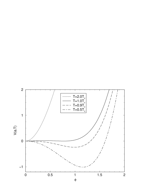
Figure 1: Interaction potential $V(\phi,~{}T)$ (equation (2) in the text) as a function of scalar field at four different temperatures $T/T_{c}=(2,~{}1,~{}0.9,~{}0.5)$. The potential parameters used here are: surface tension $\sigma=0.1~{}T_{c}$, correlation length $\ell_{c}=1.0/T_{c}$, latent heat $L=2.0~{}T_{c}^{4}$, and critical temperature $T_{c}=1$.

The resulting differential equations for momentum and energy, neglecting baryon conservation, can be written in flux conservative form as

$$\partial_{t}S_{j}+{\partial_{i}}(S_{j}v^{i}) = -\partial_{j}[p_{r}-V(\phi,~{}T)]-\left[\kappa W\partial_{t}\phi+\kappa Wv^{i}\partial_{i}\phi+\partial_{\phi}V(\phi,~{}T)\right]\partial_{j}\phi~{},$$ (5)

$$\partial_{t}E+{\partial_{i}}(Ev^{i}) = -[p_{r}-V(\phi,~{}T)][\partial_{t}W+{\partial_{i}}(Wv^{i})]$$ (6)

$$+\kappa(W\partial_{t}\phi+Wv^{i}\partial_{i}\phi)^{2}+\partial_{\phi}V(\phi,~{}T)(W\partial_{t}\phi+Wv^{i}\partial_{i}\phi)~{},$$

which, together with the scalar field wave equation,

$$\partial^{2}_{t}\phi-\partial^{i}\partial_{i}\phi=-\partial_{\phi}V(\phi,~{}T)-\kappa W(\partial_{t}\phi+v^{i}\partial_{i}\phi)~{},$$ (7)

and a prescription for the equation of state described below, represent the complete system of equations we solve in this paper. In deriving the above equations, we have implicitly assumed a flat space metric, and defined variables so that $W=u^{0}=1/\sqrt{1-v^{i}v_{i}}$ is the relativistic boost factor, $v^{i}=u^{i}/u^{0}$ is the transport velocity, $S_{i}=W\rho hu_{i}$ is the covariant momentum density, $E$ is the generalized internal energy density

$$\frac{E}{W}=3a_{r}T^{4}+V(\phi,~{}T)-T\partial_{T}V(\phi,~{}T)~{},$$ (8)

$a_{r}=g_{*}(\pi^{2}/90)$ is a radiation constant defining the particle content and degrees of freedom $g_{*}$, and $\kappa$ is a constant coefficient regulating entropy production and kinematic and scalar field energy dissipation. The terms associated with $\kappa$ act as an effective friction force at the phase transition surface boundary Ignatius et al. (1994); Kurki-Suonio and Laine (1996).

The hydrodynamic equations are solved using the Cosmos code Anninos and Fragile (2003); Anninos et al. (2002) with time-explicit operator split methods, second order spatial finite differencing, and artificial viscosity to capture shocks Wilson (1979). The scalar field wave equation is solved using a second order (in space and time) predictor-corrector integration, sub-cycling within a single hydrodynamic cycle since equation (7) generally has a tighter restriction on the time step for stability.

A second formulation of the dynamical equations considered here is based on a simpler conservative hyperbolic description of the hydrodynamics equations. In this case, the equations are derived directly by expanding the conservation of stress-energy $T^{\mu\nu}_{\ \ ,\nu}=0$ into time and space explicit parts. In flat space, this yields the same equations (5) and (7) for momentum conservation and scalar field evolution, but with

$$\partial_{t}{\cal E}+{\partial_{i}}({\cal E}v^{i})=-{\partial_{i}}[v^{i}(p_{r}-V(\phi,~{}T))]+\left[\kappa W\partial_{t}\phi+\kappa Wv^{i}\partial_{i}\phi+\partial_{\phi}V(\phi,~{}T)\right]\partial_{t}\phi$$ (9)

in place of (6) for the energy variable, defined as

$${\cal E}=W\rho hu^{0}-[p_{r}-V(\phi,~{}T)].$$ (10)

The Cosmos code uses a non-oscillatory central difference numerical scheme Jiang et al. (1998) with second order spatial differencing and predictor-corrector time integration with dimensional splitting to solve the hydrodynamics equations in this formalism. Artificial viscosity is not needed in this approach. Instead, shocks are captured with MUSCL-type piece-wise linear interpolants and high order limiters for flux reconstruction, but without the complexity of Riemann solvers.

A final ingredient needed is an equation of state relating $p_{r}$ to energy $E$ and temperature $T$. Here we assume $p_{r}=a_{r}T^{4}$, treating the plasma as a gas of relativistic particles with enthalpy density

$$\rho h=\frac{\gamma p_{r}}{\gamma-1}-T\partial_{T}V(\phi,~{}T)=4a_{r}T^{4}-T\partial_{T}V(\phi,~{}T)=\frac{E}{W}+p_{r}-V(\phi,~{}T)~{},$$ (11)

and adiabatic index $\gamma=4/3$. The equation of state is then written in terms of computed quantities

$$p_{eff}=p_{r}-V(\phi,~{}T)=(\gamma-1)\left(\frac{E}{W}+T\partial_{T}V(\phi,~{}T)-V(\phi,~{}T)\right)-V(\phi,~{}T)~{},$$ (12)

or

$$p_{eff}=p_{r}-V(\phi,~{}T)=(\gamma-1)\left(\frac{{\cal E}-V(\phi,~{}T)+TW^{2}\partial_{T}V(\phi,~{}T)}{\gamma W^{2}-(\gamma-1)}\right)-V(\phi,~{}T)~{},$$ (13)

depending on which energy variable is evolved. The quantity $p_{eff}$ is introduced as an effective pressure for numerical convenience in solving equations (5), (6) and/or (9). The fluid temperature is computed from either

$$\frac{E}{W}-3a_{r}T^{4}-V(\phi,~{}T)+T\partial_{T}V(\phi,~{}T)=0~{},$$ (14)

or

$${\cal E}-V(\phi,~{}T)+TW^{2}\partial_{T}V(\phi,~{}T)-3a_{r}T^{4}[\gamma W^{2}-(\gamma-1)]=0~{}.$$ (15)

Equations (14) and (15) are solved using a Newton-Raphson method to iterate and converge on the temperature, assuming an initial guess of $T_{0}=(E/3Wa_{r})^{1/4}$.

III Perturbation Analysis

In this section we carry out a first-order perturbation expansion of the hydrodynamics equations, and review briefly the expected dynamical behavior and stability of phase transitions in the context of linear theory. The general aproach follows that presented in references Link (1992); Kamionkowski and Freese (1992); Huet et al. (1993); Abney (1994). In addition to elucidating any unstable behavior, the results of this section are also used to set up inhomogeneous perturbations as initial data that is evolved numerically in §IV.

It is convenient to start with the hydrodynamics equations in conservative hyperbolic form (5) and (9), which we rewrite here as

$$\partial_{t}{\cal E}+\partial_{i}({\cal E}v^{i}+v^{i}p) = \Sigma^{0}~{},$$ (1)

$$\partial_{t}S^{j}+\partial_{i}(S^{j}v^{i}+\delta_{ij}p) = \Sigma^{j}~{},$$ (2)

assuming a constant scalar field potential on either side of the phase transition front, and $\Sigma^{0}$ and $\Sigma^{j}$ represent any source or dissipative terms. Equations (1) and (2) are expanded out to first perturbative order assuming two dimensional perturbations off a homogeneous background flow of the form

$$p = p_{0}+\delta p(t,x,y)~{},$$ (3)

$${\bf v} = v_{0}~{}\widehat{i}+[\delta v_{x}(t,x,y)~{}\widehat{i}+\delta v_{y}(t,x,y)~{}\widehat{j}]~{},$$ (4)

for the fluid pressure and velocity. The corresponding boost factor and conserved variables are, to first order

$$W = \frac{1}{\sqrt{1-v^{2}}}=\frac{1}{\sqrt{1-v_{0}^{2}}}+\frac{v_{0}}{(1-v_{0}^{2})^{3/2}}~{}\delta v_{x}~{},$$ (5)

$${\cal E} = \frac{p(\gamma W^{2}-\gamma+1)}{\gamma-1}=-p_{0}+\frac{\gamma p_{0}}{(\gamma-1)(1-v_{0}^{2})}$$ (6)

$$\hskip 85.0pt+\frac{2\gamma p_{0}v_{0}}{(\gamma-1)(1-v_{0}^{2})^{2}}~{}\delta v_{x}+\frac{\gamma}{(\gamma-1)(1-v_{0}^{2})}~{}\delta p-\delta p~{},$$

$$S^{x} = \frac{\rho hv^{x}}{1-v^{2}}=\frac{\gamma}{(\gamma-1)(1-v_{0}^{2})}\left(p_{0}v_{0}+p_{0}~{}\delta v_{x}+v_{0}~{}\delta p+\frac{2p_{0}v_{0}^{2}}{1-v_{0}^{2}}~{}\delta v_{x}\right)~{},$$ (7)

$$S^{y} = \frac{\rho hv^{y}}{1-v^{2}}=\frac{\gamma p_{0}}{(\gamma-1)(1-v_{0}^{2})}~{}\delta v_{y}~{},$$ (8)

where $\rho h=(e+p)=\gamma p/(\gamma-1)$, and $v_{0}$ is the unperturbed fluid velocity.

Substituting (5) - (8) into (1) and (2) yields for momentum conservation along the $y$-axis

$$\partial_{y}(\delta p)+\frac{\gamma p_{0}}{(\gamma-1)(1-v_{0}^{2})}\left[\partial_{t}(\delta v_{y})+v_{0}\partial_{x}(\delta v_{y})\right]=\Sigma^{y}~{},$$ (9)

for momentum conservation along the $x$-axis

$$(\gamma-1)(1-v_{0}^{2})\Sigma^{x} = \gamma v_{0}~{}\partial_{t}(\delta p)+\gamma p_{0}(1+v_{0}^{2})(1-v_{0}^{2})^{-1}~{}\partial_{t}(\delta v_{x})$$ (10)

$$+ (\gamma-1+v_{0}^{2})~{}\partial_{x}(\delta p)+2\gamma p_{0}v_{0}(1-v_{0}^{2})^{-1}~{}\partial_{x}(\delta v_{x})+\gamma p_{0}v_{0}~{}\partial_{y}(\delta v_{y})~{},$$

and for energy conservation

$$(\gamma-1)(1-v_{0}^{2})\Sigma^{0} = \left(1-v_{0}^{2}+\gamma v_{0}^{2}\right)~{}\partial_{t}(\delta p)+2\gamma p_{0}v_{0}(1-v_{0}^{2})^{-1}~{}\partial_{t}(\delta v_{x})$$ (11)

$$+ \gamma v_{0}~{}\partial_{x}(\delta p)+\gamma p_{0}(1+v_{0}^{2})(1-v_{0}^{2})^{-1}~{}\partial_{x}(\delta v_{x})+\gamma p_{0}~{}\partial_{y}(\delta v_{y})~{},$$

all to first perturbative order.

Equations (10) and (11) can be simplified further by first eliminating $\partial_{y}(\delta v_{y})$ from the $x$-momentum equation

$$0 = (\gamma-1)(1-v_{0}^{2})\left(\Sigma^{x}-v_{0}\Sigma^{0}\right)$$ (12)

$$= v_{0}\partial_{t}(\delta p)+\rho h_{0}W_{0}^{2}\partial_{t}(\delta v_{x})+\partial_{x}(\delta p)+W_{0}^{2}\rho h_{0}v_{0}\partial_{x}(\delta v_{x})~{},$$

then eliminating $\partial_{t}(\delta v_{x})$ from the energy equation

$$0 = c_{s}^{2}(\gamma-1)(1-v_{0}^{2})\left[\Sigma^{0}-\left(\frac{2v_{0}}{1+v_{0}^{2}}\right)\Sigma^{x}\right]$$ (13)

$$= (1-v_{0}^{2}c_{s}^{2})\partial_{t}(\delta p)+v_{0}(1-c_{s}^{2})\partial_{x}(\delta p)+\rho h_{0}\left[\partial_{x}(\delta v_{x})+\partial_{y}(\delta v_{y})\right]~{}.$$

In writing (12) and (13) we introduced the notation $c_{s}^{2}=\gamma-1$, $W_{0}^{2}=1/(1-v_{0}^{2})$ $\rho h_{0}=\gamma p_{0}/(\gamma-1)$, and explicitly ignored the source terms $\Sigma^{\alpha}$ by setting them to zero.

The final equations (9), (12), and (13) can be written conveniently in compact form as

$${\bf A_{t}}\partial_{t}{\bf W}+{\bf A_{x}}\partial_{x}{\bf W}+{\bf A_{y}}\partial_{y}{\bf W}=0~{},$$ (14)

where ${\bf W}=(\delta p,~{}\delta v_{x},~{}\delta v_{y})$, and

$${\bf A_{t}} = \left(\begin{array}[]{lll}1-v_{0}^{2}c_{s}^{2}&0&0\\ v_{0}&\rho h_{0}W_{0}^{2}&0\\ 0&0&\rho h_{0}W_{0}^{2}\end{array}\right)~{},$$ (18)

$${\bf A_{x}} = \left(\begin{array}[]{lll}v_{0}(1-c_{s}^{2})&\rho h_{0}c_{s}^{2}&0\\ 1&W_{0}^{2}\rho h_{0}v_{0}&0\\ 0&0&\rho h_{0}W_{0}^{2}v_{0}\end{array}\right)~{},$$ (22)

$${\bf A_{y}} = \left(\begin{array}[]{lll}0&0&\rho h_{0}c_{s}^{2}\\ 0&0&0\\ 1&0&0\end{array}\right)~{}.$$ (26)

Next, following the general procedure outlined in reference Abney (1994), we assume a solution of the form ${\bf W}(t,x,y)={\bf w}(x)e^{-i(\omega t+ky)}$, with ${\bf w}(x)=\sum a_{j}e^{-i\lambda^{*}_{j}x}{\bf R_{j}}$ and the following characteristic equation or dispersion relation for (14):

$$(\omega+\lambda^{*}v_{0})[k^{2}(1-v_{0}^{2})-c_{s}^{-2}(\omega+\lambda^{*}v_{0})^{2}+(\lambda^{*}+\omega v_{0})^{2}]=0~{}.$$ (27)

Equation (27) has either three distinct roots which agree with those found by Huet et al. (1993); Abney (1994)

$$\lambda^{*}_{1} = -\frac{\omega}{v_{0}}~{},$$ (28)

$$\lambda^{*}_{\pm} = \frac{1}{v_{0}^{2}-c_{s}^{2}}\left[(c_{s}^{2}-1)v_{0}\omega\pm c_{s}(1-v_{0}^{2})\sqrt{\omega^{2}+\frac{v_{0}^{2}-c_{s}^{2}}{1-v_{0}^{2}}~{}k^{2}}\right]~{},$$ (29)

or two roots

$$\lambda^{*}_{1} = -\frac{\omega}{c_{s}}~{},$$ (30)

$$\lambda^{*}_{2} = \frac{v_{0}k^{2}}{2\omega}-\frac{\omega(1+v_{0}^{2})}{2v_{0}}~{},$$ (31)

if $v_{0}=c_{s}$. The corresponding eigenvectors of (14) are

$${\bf R_{1}} = \left(\begin{array}[]{l}0\\ kv_{0}/\omega\\ 1\end{array}\right)~{},$$ (35)

$${\bf R_{-}} = \left(\begin{array}[]{l}\left(\rho h_{0}\omega c_{s}^{2}+\rho h_{0}v_{0}c_{s}\Omega\right)/(k(v_{0}^{2}-c_{s}^{2}))\\ \left(v_{0}\omega+c_{s}\Omega\right)(1-v_{0}^{2})/(k(c_{s}^{2}-v_{0}^{2}))\\ 1\end{array}\right)~{},$$ (39)

$${\bf R_{+}} = \left(\begin{array}[]{l}\left(\rho h_{0}\omega c_{s}^{2}-\rho h_{0}v_{0}c_{s}\Omega\right)/(k(v_{0}^{2}-c_{s}^{2}))\\ \left(v_{0}\omega-c_{s}\Omega\right)(1-v_{0}^{2})/(k(c_{s}^{2}-v_{0}^{2}))\\ 1\end{array}\right)~{},$$ (43)

where we define $\Omega=[\omega^{2}+k^{2}(v_{0}^{2}-c_{s}^{2})/(1-v_{0}^{2})]^{1/2}$ in equations (39) and (43).

To determine whether any unstable modes of ${\bf W}$ exist and are consistent with imposed boundedness conditions at $x\rightarrow\pm\infty$, it is convenient to construct a coordinate system centered and moving with the frame of the interface between quark and hadron phases at $x=0$. Assuming the high temperature quark phase is to the left of the interface ($x<0$), and the hadron phase to the right ($x>0$), we can easily determine if any unstable modes (defined by Im$(\omega)>0$) obey the conditions ${\bf W}\rightarrow 0$ as $x\rightarrow\pm\infty$. As concluded in references Huet et al. (1993); Abney (1994), if Im$(\omega)>0$ in the quark region of a detonation front, then Im$(\lambda_{j}^{*})<0$ and therefore $a_{j}=0$ for all $j$ in order for the solutions to be bounded at $x\rightarrow-\infty$. Hence unstable modes do not exist in regions ahead of nucleating bubbles separated from the quark phase by a detonation front. However, in the hadron region to the right ($x>0$) of a detonation front, the boundedness conditions at $x\rightarrow+\infty$ do not rule out unstable modes to linear order. Also, in the case of deflagration fronts, unstable modes are realizable on both the quark and hadron sides, at least for cases in which surface tension, dissipation, and strong thermal coupling effects are negligible Link (1992); Huet et al. (1993); Kamionkowski and Freese (1992). It is not entirely clear what role these effects play in stabilizing the transition, and certainly higher order nonlinear effects are not accounted for in this analysis. Table 1 summarizes which of the regions and hydrodynamic states may potentially give rise to unstable modes with $\mbox{Im}(\omega)>0$, at least to linear order.

Table 1: Summary of parameters yielding bound solutions that are susceptible to unstable modes. The entries represent a general set of conditions that allow unstable modes ($\mbox{Im}(\omega)>0$) to first perturbative order for each of the phases and front types. These conditions are used to construct initial data for the multi-dimensional numerical stability studies presented in section §IV.

Quark region ($x<0$)	Hadron region ($x>0$)
detonations:	detonations:
$v_{q}>c_{s}$	$v_{h}<v_{q}$
$a_{1}=0$	$\lambda^{*}_{1}=-\omega/v_{0}$
$a_{-}=0$	$a_{-}=0$
$a_{+}=0$	Im$(\lambda^{*}_{+})<0$
deflagrations:	deflagrations:
$v_{q}<c_{s}$	$v_{h}>v_{q}$
$a_{1}=0$	$\lambda^{*}_{1}=-\omega/v_{0}$
Im$(\lambda^{*}_{-})>0$	$a_{-}=0$
$a_{+}=0$	Im$(\lambda^{*}_{+})<0$

IV Numerical Results

IV.1 Initial Data

The initial data has just one free dimension, energy, which we use to specify the critical transition temperature $T_{c}$ and normalize it to unity. It is also convenient to define a characteristic length scale as the radius of a spherical nucleated hadron bubble in approximate equilibrium with an exterior quark plasma. This is estimated by balancing pressure forces acting from the quark and hadron sides and including the effect of surface tension, resulting in $R_{eq}=2\sigma/(p_{h}-p_{q})$ for the equilibrium radius, where $\sigma$ is the surface tension, and $p_{h}$ and $p_{q}$ are the pressure fields from the hadron and quark sides respectively. For the preliminary one-dimensional calculations in §IV.2, the computational box sizes are set to a multiple of the equilibrium bubble radius $L=xR_{eq}$, with $x$ generally in the range 20 - 2000. Typical length scales or box sizes in these calculations vary from a few hundred to a few thousand fermi. By comparison, the proper horizon size at the time of the QCD phase transition is

$$d_{H}=2t_{age}=R(t)\int_{0}^{t}dt^{\prime}/R(t^{\prime})=\frac{16}{\sqrt{g_{*}/51.25}~{}(T_{MeV}/150~{}\mbox{MeV})^{2}}~{}\mbox{km}~{},$$ (1)

or 16 km for $g_{*}=51.25$ and $T_{MeV}=150~{}\mbox{MeV}$. In writing (1) we have assumed $R(t)$ is the cosmological scale factor in the isotropic FLRW background model dominated by radiation energy density of the form $e=a_{r}T^{4}=e_{0}R^{-2}$ such that

$$t_{age}=\sqrt{\frac{3c^{2}}{32\pi Ga_{r}}}~{}T^{-2}=\frac{2.7\times 10^{-5}}{\sqrt{g_{*}/51.25}~{}(T_{MeV}/150\mbox{MeV})^{2}}~{}\mbox{s}$$ (2)

is the age of the Universe as a function of temperature.

We consider two background temperatures for the super-cooled initial state triggering the shock and phase front propagation: $T=0.9T_{c}$ and $T=0.9943T_{c}$. The latter temperature is chosen to match the 1+1 dimensional cases considered in reference Ignatius et al. (1994), and provides a useful benchmark against which some of our results can be compared.

To keep the number of numerical simulations down to a reasonable level, we fix the following additional parameters for all calculations and for both temperature cases: critical transition temperature $T_{c}=150$ MeV corresponding to the QCD symmetry breaking energy occurring when the Universe was approximately $t_{age}=2.7\times 10^{-5}$ s old (see equation (2)); particle degrees of freedom $g_{*}=51.25$ to be consistent with previous studies Kajantie and Kurki-Suonio (1986); surface tension $\sigma=0.1~{}T_{c}$; correlation length $\ell_{c}=1.0/T_{c}$; and latent heat $L=2~{}T_{c}^{4}$. Note that for both temperatures considered here, the interaction potential (equation (2) and Figure 1) has two local minima (at $\phi=0$ and $\phi=\phi_{min}(T)>0$, which allows for the quark (cold phase with $\phi=0$) and hadron (hot phase with $\phi=\phi_{min}(T)$) states to co-exist.

The remaining parameter, the dissipation constant $\kappa$, is varied over the range $0.1\leq\kappa\leq 10$ in the one-dimensional calculations to determine the regimes in which detonations and deflagrations are triggered, and to compute the stability parameters from linear theory.

The scalar field $\phi$ is initialized according to Ignatius et al. (1994)

$$\phi(x)=\phi_{c}(1+\Delta)\frac{2\alpha T\overline{\lambda}}{3\lambda}\left(\frac{1-\sqrt{1-f(L-x)}}{f(L-x)}\right)~{},$$ (3)

with

$$f(x)=\frac{1-\overline{\lambda}\coth^{2}(\sqrt{\beta(T^{2}-T_{0}^{2})}~{}x/(1+\Delta))}{1-\coth^{2}(\sqrt{\beta(T^{2}-T_{0}^{2})}~{}x/(1+\Delta))}~{},$$ (4)

$\overline{\lambda}=9\lambda\beta(T^{2}-T_{0}^{2})/(2\alpha^{2}T^{2})$, and $x=L$ is the right-most edge along the $x$-axis representing the computational box size. These expressions define a hadron phase with $\phi>0$ at $L-x\rightarrow 0$, and quark phase with $\phi\rightarrow 0$ as $L-x\rightarrow\infty$, with an exponentially steep interface boundary of width set by the model parameters. The numerical constants $\phi_{c}$ and $\Delta=0.05$ are used to perturb the solution out of dynamical equilibrium by varying both the amplitude and width of the field in the hadron phase. For most of the calculations we set $\phi_{c}=1$. However, for the larger $\kappa$ cases we found it useful to specify $\phi_{c}$ such that $\phi(x=L)\approx\phi_{min}(T)$, in order to reduce the transient interval between the initial configuration and the time that the phase front fully develops.

IV.2 One-Dimensional Results

The primary motivations for the one-dimensional calculations presented here were to narrow the parameter space and help illuminate the two-dimensional studies presented in the following section for the different background temperatures considered. In cases where the temperature was initialized to $T=0.9T_{c}$, we used anywhere from $2\times 10^{3}$ to $3.2\times 10^{4}$ zones to resolve a length scale of $L=2000R_{eq}=2190$ fm. For runs in which $T=0.9943T_{c}$ we used from $5\times 10^{2}$ to $4\times 10^{3}$ zones to resolve $L=20R_{eq}=452$ fm. In these 1D parameter studies, we also considered an initial background temperature of $T=0.95T_{c}$. These runs were useful for characterizing some of the intermediate states in the 2D runs below. For these $T=0.95T_{c}$ runs we used from $1\times 10^{3}$ to $4\times 10^{3}$ zones to resolve $L=250R_{eq}=1157$ fm. The higher resolutions in each temperature case were generally required for the larger values of $\kappa$ in order to maintain reasonable zone coverage in the hadron phase, since the bubble growth velocity was sometimes substantially less than the shock front velocity, or near the transition from a detonation front to a deflagration front, as detailed below. For this first group of 1D runs, the code was allowed to run for approximately one sound-crossing time $t_{s}=L/c_{s}$, where $c_{s}=1/\sqrt{3}$.

Figure 2 shows the phase front or bubble growth velocity normalized to the sound speed $v_{f}/c_{s}$, and the quantity $\eta=-T_{c}v_{f}dv_{f}/dT_{q}$ as a function of the dissipation parameter $\kappa$ for temperatures $T/T_{c}=0.9$, $0.95$, and $0.9943$. According to reference Huet et al. (1993), $\eta$ determines the stability of bubbles and we compute it using the approximation $\eta=v_{f}^{2}/v_{c}^{2}$, where $v_{c}^{2}=(1/2)(1-T_{q}^{2}/T_{c}^{2})$. Notice the $T=0.9T_{c}$ curve switches from a detonation to a deflagration at $\kappa\approx 1$ where $v_{f}/c_{s}$ crosses unity, and the $T=0.95T_{c}$ curve switches at $\kappa\approx 0.3$. However, the precise transition points are highly sensitive to the resolution and duration of the simulations, and what might appear as a deflagration at one resolution may turn out to be a detonation at another. This is attributed to the solutions approaching either a Jouget or temporary strong detonation state (which eventually decays into a weak deflagration) as the parameter $\kappa$ is increased. In particular, the post-shock velocity for the $T=0.9T_{c}$ case computed over short time intervals in the frame of the front decreases from being supersonic at low values of $\kappa$, to about sonic speed at $\kappa=0.875$, then subsonic at higher values but less than unity (e.g., $\kappa=0.9$), corresponding to weak, nearly Jouget, and strong detonations, respectively. Solutions for which $\kappa$ is close to unity thus represent a regime in parameter space that does not allow stable detonation modes since strong detonations are forbidden modes of propagation (see, for example, Kurki-Suonio and Laine (1995)). We note that the conservative hyperbolic form of the hydrodynamics equations and the non-oscillatory central difference methods for solving the equations generally out-perform artificial viscosity methods in resolving and maintaining stable evolutions near the critical Jouget state.

Figure 2: Bubble growth velocity normalized to the sound speed $v_{f}/c_{s}$, and stability parameter $\eta$ as a function of the dissipation constant $\kappa$ for temperatures $T/T_{c}=0.9$, $0.95$, and $0.9943$. The $T=0.9T_{c}$ ($T=0.95T_{c}$) curve switches from a detonation to a deflagration at $\kappa\approx 1$ ($\kappa\approx 0.3$).

Table 2 summarizes our results for the potentially unstable, $\eta<1$, deflagration runs. $T_{h}$ and $T_{q}$ in Table 2 are the average temperatures of the hadron and quark phases, respectively; and $v_{h}$ and $v_{q}$ are the hadron and quark velocities on either side of the phase front as measured in the rest frame of the moving front. The critical wave number, $k_{c}=(\mu-1)\rho h_{q}v_{q}^{2}/\sigma$, defines the limit above which the system is stabilized by surface tension Link (1992), where $\mu=v_{h}/v_{q}$ and $\rho h_{q}$ is the enthalpy density of the quark phase. Modes with wavelengths $\lambda<\lambda_{c}=k_{c}^{-1}$ are thus expected to be stable. The instability growth timescale, $\tau$, is estimated as Link (1992)

$$\frac{1}{\tau}=\frac{\mu}{1+\mu}\left[-1+\left(1+\mu-\frac{1}{\mu}-\frac{1+\mu}{\mu}\frac{\sigma k_{0}}{\rho h_{q}v_{q}^{2}}\right)^{1/2}\right]k_{0}v_{q}~{},$$ (5)

where

$$k_{0}=\frac{2}{9}\left(\frac{\mu}{1+\mu}\right)\left[2+3\mu-\frac{3}{\mu}-\left(4+3\mu-\frac{3}{\mu}\right)^{1/2}\right]\frac{\rho h_{q}v_{q}^{2}}{\sigma}$$ (6)

is the wave number of the mode with the shortest growth time scale.

Table 2: Hadron temperature $T_{h}$, quark temperature $T_{q}$, front velocity $v_{f}$, hadron velocity relative to front $v_{h}$, quark velocity relative to front $v_{q}$, critical stability wavenumber $k_{c}$, fastest growth wavenumber $k_{0}$, linear perturbation growth time $\tau$, and stability parameter $\eta$ as a function of dissipation constant $\kappa$ for initial temperatures $T/T_{c}=0.9$, $0.95$, and $0.9943$. The results are shown only for the potentially unstable 1D deflagration runs in Figure 2 that satisfy $\eta<1$.

$T/T_{c}$	$\kappa$	$T_{h}/T_{c}$	$T_{q}/T_{c}$	$|v_{f}/c_{s}|$	$v_{h}$	$v_{q}$	$k_{c}$	$k_{0}$	$\tau$	$\eta$
0.9	5.0	0.90639	0.92971	0.431	0.249	0.193	1.816	0.933	$8.25\times 10^{1}$	0.911
	6.0	0.90378	0.92449	0.364	0.210	0.164	1.250	0.642	$1.46\times 10^{2}$	0.608
	7.0	0.90275	0.92264	0.339	0.196	0.153	1.071	0.550	$1.83\times 10^{2}$	0.516
	10.0	0.89914	0.91717	0.260	0.150	0.118	0.613	0.314	$4.17\times 10^{2}$	0.285
0.95	5.0	0.95436	0.96233	0.258	0.149	0.127	0.546	0.278	$6.81\times 10^{2}$	0.602
	7.0	0.95246	0.95964	0.203	0.117	0.100	0.331	0.170	$1.43\times 10^{3}$	0.348
	10.0	0.95072	0.95747	0.158	0.091	0.077	0.198	0.101	$3.09\times 10^{3}$	0.199
0.9943	1.5	0.99633	0.99686	0.082	0.048	0.043	0.043	0.022	$4.33\times 10^{4}$	0.722
	2.0	0.99596	0.99646	0.071	0.041	0.037	0.031	0.016	$7.06\times 10^{4}$	0.479
	3.5	0.99527	0.99576	0.043	0.025	0.022	0.012	0.006	$2.66\times 10^{5}$	0.145
	5.0	0.99491	0.99541	0.033	0.019	0.016	0.007	0.004	$6.82\times 10^{5}$	0.077
	10.0	0.99439	0.99492	0.016	0.009	0.007	0.002	0.001	$5.95\times 10^{6}$	0.017

Table 3 summarizes the results computed for the detonation cases with temperature $T=0.9T_{c}$. Here $v_{f}$ represents both the front and shock velocities, and $\rho h_{h}$ is the enthalpy density of the hadrons immediately behind the phase front. The quantity $\sigma/\rho h$ has dimensions of length, and provides a natural scale that gauges the relative importance of surface tension. It is also applied as a dimensional scaling variable in the calculations of reference Abney (1994), which we use as a guide to estimate perturbation growth rates and physical run times for the two-dimensional calculations presented in §IV.3.

Table 3: Front velocity $v_{f}$ and enthalpy to surface tension ratio $(\rho h_{h})/\sigma$ on the hadron side as a function of dissipation constant $\kappa$ for a selected set of 1D detonations with initial temperature $T=0.9T_{c}$

$T/T_{c}$	$\kappa$	$|v_{f}/c_{s}|$	$(\rho h_{h})/\sigma$
0.9	0.1	1.85	191.7
	0.3	1.71	195.7
	0.5	1.57	201.1
	0.75	1.36	216.2
	0.8	1.33	220.4

In Figures 3-5, we present more detailed results of three particular 1D runs that will help illuminate the 2D calculations with similar parameters presented in the next section. Figure 3 shows a series of outputs of the scalar field and temperature for a weak (subsonic post-front velocity relative to the phase front) deflagration case with $T=0.9T_{c}$ and $\kappa=7$. This run used 2000 zones to resolve a length scale of $L=1095$ fm, and was allowed to run for slightly longer than two sound-crossing times so that the shock leading the deflagration front propagates across the grid twice. These tiled displays show a leading shock front (in the temperature graphs) originating from the right and traveling to the left with velocity slightly higher than sound speed $v_{s}=1.03c_{s}$, heating up the quarks just ahead of the cool hadron phase (first row). The deflagration front (separating the two regions with different scalar field values) travels to the left at a speed slower than the leading shock front, $v_{f}/c_{s}\approx 0.34$. Due to the reflection boundary conditions imposed on all our calculations, a mirrored shock collision occurs when the leading shock hits the left boundary (second row). The reflected shock then travels to the right, eventually colliding with the phase front moving in the opposite direction (third row). The shock heats up the fluid and reduces the scalar field as it passes through the hadron phase. Upon impact with the phase front, the shock/front interaction also generates a rarefaction wave traveling to the left which cools off the quarks in its path. Finally the hadron matter at the right end is heated further as the reflected shock hits the right boundary and collides with another incoming shock (fourth row).

Figure 3: Scalar field (left column) and temperature (right column) as a function of position for a 1D deflagration case with $T=0.9T_{c}$ and $\kappa=7$. Top row: Early undisturbed deflagration and shock fronts at $t=3.2\times 10^{-21}$ s. Second row: Shock collision in the quark phase at the left boundary at $t=6.6\times 10^{-21}$ s. Third row: Reflected shock interacting with deflagration front at $t=1.1\times 10^{-20}$ s. Fourth row: Interaction of two reflected shocks in the hadron phase at the right boundary at $t=1.4\times 10^{-20}$ s.

Figure 4 shows a similar series of displays for a weak (supersonic post-shock velocity relative to the phase front) detonation case with $T=0.9T_{c}$ and $\kappa=0.5$, run for almost two sound-crossing times. This run used 2000 zones to resolve a length scale of $L=1095$ fm. The outputs begin in the first row with an early undisturbed state showing the leading shock/detonation front originating at the right end of the grid and traveling to the left at speed $v_{f}/c_{s}\approx 1.6$. A rarefaction wave follows the shock and separates two hadron regions at two slightly different temperatures. The second row shows the shock-shock collision which occurs when the leading shock front reaches and reflects off the left boundary. This interaction heats up the fluid to temperatures higher than $T_{c}$, and generates a quark region at the left boundary. As the reflected shock travels to the right, the quark region grows. The third row shows the reflected shock passing through the rarefaction wave separating the two hadron states. This rarefaction wave cools the newly formed quark region, converting quarks back into hadrons. The fourth row shows the interaction of reflected rarefaction waves at the left boundary. The complete reflected state showing the thermal distortion and shock profiles after the entire domain is converted to the hadron phase is displayed in the fifth row. This compact structure is allowed to traverse the grid and interact through each sequence again at the right boundary (sixth row). The complete reflected state from the right boundary is shown in the final row.

Figure 4: Scalar field (left column) and temperature (right column) as a function of position for a 1D detonation case with $T=0.9T_{c}$ and $\kappa=0.5$. Top row: Early undisturbed detonation front plus rarefaction at $t=2.2\times 10^{-21}$ s. Second row: Shock-shock interaction at left boundary at $t=4.8\times 10^{-21}$ s. Third row: Reflected shock passing through the rarefaction wave at $t=5.7\times 10^{-21}$ s. Fourth row: Interaction of the rarefaction waves at left boundary at $t=6.6\times 10^{-21}$ s. Fifth row: Reflected state from left boundary at $t=9.7\times 10^{-21}$ s. Sixth row: Interaction of reflected states at right boundary at $t=1.2\times 10^{-20}$ s. Seventh row: Reflected state from right boundary at $t=1.5\times 10^{-20}$ s.

Figure 5 shows outputs from two phase front systems originating in separate regions at different temperatures and are thus out of initial thermal equilibrium: a deflagration front at $T=0.9943T_{c}$ at the left end, and a detonation front at $T=0.9T_{c}$ at the right end. This run used 2000 zones to resolve a length scale of $L=1806.1$ fm. The dissipation constant is $\kappa=0.5$ across both regions, and the temperature discontinuity is initiated at the center of the grid. The right end is initialized to the same state as the previous detonation case in Figure 4. The left end is similar to the weak deflagration case of Figure 3, but with a smaller dissipation constant and a higher initial temperature. The first row illustrates an early stage where the deflagration front has formed at the left end with $v_{f}/c_{s}\approx 0.14$, the shock/detonation front and rarefaction wave have formed at the right end with $v_{s}=v_{f}\approx 1.6c_{s}$, and a thermal shock front and rarefaction wave are traveling in opposite directions from the central thermal discontinuity at about the sound speed. The second row shows the collision of the detonation and thermal shocks. The third row shows the passage of the thermal shock through the detonation rarefaction, and the collision of the deflagration shock with the thermal rarefaction wave. The fourth row shows the interaction of the deflagration front with the thermal rarefaction at the left end, and the collision of the deflagration and detonation shocks at the middle. As the rarefaction wave passes through the hadron phase behind the deflagration front at the left end, the phase transition is accelerated to near sound speed. The fifth row shows the accelerated shock and deflagration front features traveling to the right at velocities $v_{s}\approx 0.67=1.16c_{s}$ and $v_{f}\approx 0.51=0.88c_{s}$. Notice that the accelerated front velocity is close to, but slightly faster than the deflagration velocity predicted by the $T=0.95T_{c}$ curve of Figure 2, which yields $v_{f}=0.74c_{s}=0.43$. The sixth row shows the interaction of the newly accelerated front with the detonation propagating from the right end. This interaction heats up and decomposes the hadrons back into quarks over a substantially large region at the center. The newly formed quark region gradually cools with the shock passage and rarefaction wave interactions. Profiles and distributions of quark and hadron regions become increasingly complex as indicated in the final row due to the various shock, phase, and sound wave interactions as they reflect off the boundaries and propagate through the grid.

Figure 5: Scalar field (left column) and temperature (right column) as a function of position for a 1D interaction of shocks and phase fronts originating in two separate regions at different temperatures: a deflagration system at $T=0.9943T_{c}$ at the left end, and a detonation configuration at $T=0.9T_{c}$ at the right end. The dissipation constant is $\kappa=0.5$ everywhere, and the temperature discontinuity is initiated at the grid center at $t=0$. Top row: Early undisturbed deflagration and shock fronts (left), detonation front plus rarefaction (right), and thermal shock front plus rarefaction (center) at $t=1.8\times 10^{-21}$ s. Second row: Interaction of detonation front and thermal shock at $t=2.2\times 10^{-21}$ s. Third row: Interaction of the detonation rarefaction and thermal shock, and thermal rarefaction and deflagration shock at $t=3.1\times 10^{-21}$ s. Fourth row: Interaction of deflagration front and thermal rarefaction, and deflagration shock and detonation shock at $t=4.8\times 10^{-21}$ s. Fifth row: Acceleration of deflagration front by thermal rarefaction at $t=5.3\times 10^{-21}$ s. Sixth row: Interaction of newly accelerated front and detonation front at $t=7.5\times 10^{-21}$ s. Seventh row: Interactions of multiple shocks resulting in two separate quark regions at $t=1.1\times 10^{-20}$ s.

We point out that, in general, Figure 2 cannot always be used to predict reliably the accelerated velocity or mode of propagation from rarefaction wave/front interactions. For example, consider the same initial configuration used in producing Figure 5, but with friction parameter $\kappa=0.2$. In this case Figure 2 predicts, for a mean field temperature $T=0.95T_{c}$, a supersonic front velocity of $v_{f}=1.56c_{s}$. However, the actual (numerical) accelerated solution remains a weak deflagration with subsonic velocity $v_{f}=0.54=0.94c_{s}$, only slightly faster than for the $\kappa=0.5$ case. This holds even in the limit $\kappa\rightarrow 0$: the accelerated front velocity approaches but does not exceed the sound speed as $\kappa\rightarrow 0$, and the propagation mode remains a deflagration with clearly separated phase and shock front features.

IV.3 Two-Dimensional Results

We focus here on extending to two dimensions several of the more interesting parameter combinations presented in section §IV.2 that may potentially give rise to unstable behavior as predicted by linear theory. In particular, we consider six calculations: runs A and B are single deflagrating fronts; run C is a single detonation transition; runs D and E are interactions between a planar and smaller spherical nucleating bubble of deflagration (run D) and detonation (run E) types; and run F is the interaction of a deflagration system with a detonation front nucleating from two regions out of thermal equilibrium. Table 4 summarizes the parameters used in each of these runs.

Table 4: Summary of parameters for the two-dimensional runs.

Run	$T/T_{c}$	$\kappa$	$\lambda_{c}$	$\tau$	Grid Dimensions		Stop Time
			(fm)	(s)	(fm)	(zones)	(s)
A	0.9	7.0	1.2	$1.3\times 10^{-21}$	$278.03\times 6.14$	$1280\times 64$	$3.2\times 10^{-21}$
B	0.9943	1.5	31.	$2.6\times 10^{-19}$	$3059.83\times 152.99$	$1280\times 64$	$7.1\times 10^{-20}$
C	0.9	0.5	6.6	$2.2\times 10^{-22}$	$302.34\times 32.71$	$1024\times 256$	$3.5\times 10^{-21}$
D	0.9	7.0	1.2	$1.3\times 10^{-21}$	$1000\times 1000$	$512\times 512$	$1.2\times 10^{-20}$
E	0.9	0.5	6.6	$2.2\times 10^{-22}$	$1000\times 1000$	$1024\times 1024$	$1.2\times 10^{-20}$
F	0.9943/0.9	0.5	$\dots$	$\dots$	$1806.1\times 451.53$	$2048\times 512$	$2.1\times 10^{-20}$

For all of these simulations we initialize the data with various perturbations included. First, the planar fronts in each problem are perturbed with a sinusoid of wavelength $\lambda\approx 5\lambda_{c}$, where $\lambda_{c}$ is the critical wavelength calculated from our 1D studies. The amplitude of this perturbation is $\delta x/x=0.05$, and the wavelength $\lambda$ is used to set the physical size of the grid parallel to the phase front.

Transverse and longitudinal inhomogeneous fluctuations are also imposed on all the initial data using the perturbation solutions discussed in §III. In particular, $E=E_{0}+\delta E$, $v_{x}=\delta v_{x}$, and $v_{y}=\delta v_{y}$, with $E_{0}=3a_{r}T^{4}+V(\phi,~{}T)-T\partial_{T}V(\phi,~{}T)$, where

$$\left(\begin{array}[]{l}(\gamma-1)\delta(E/W)\\ \delta v_{x}\\ \delta v_{y}\end{array}\right)=e^{-i(\omega t+ky)}\sum_{j}a_{j}{\bf\widetilde{R}_{j}}e^{\mbox{Im}(\lambda_{j}^{*})x}e^{-i\mbox{Re}(\lambda_{j}^{*})x}~{},$$ (7)

$\lambda_{j}^{*}$ are the eigenvalues, and ${\bf\widetilde{R}_{j}}={\bf{R}_{j}}/|{\bf{R}_{j}}|$ are the normalized eigenvectors. The expansion coefficients are defined as $a_{j}=\mbox{min}(Av_{o},~{}AE_{0})$ with amplitude constant $A=0.1$ (if they are not set to zero because of boundedness constraints as discussed in §III). $v_{0}$ is the background average velocity in either the quark or hadron regions as defined in §III, but implied here to be the velocity component orthogonal to the interface boundary and measured in the rest frame of the unperturbed surface. We take $v_{0}=c_{s}+0.5(1-c_{s})$ or $v_{0}=0.1c_{s}$ for the unperturbed velocity in the detonation or deflagration cases, respectively. Finally, we also impose random fluctuations in the background temperature with peak excursions of $\delta T/T=0.005$.

IV.3.1 Single Front Perturbations

The growth and/or decay of perturbations are tracked by calculating the power spectral density (PSD) of various wavelength modes as a function of time. Here the PSD is defined as $P(k)=2|C_{k}|^{2}/N^{2}$, where $N$ is the number of zones parallel to the front, $k=1,2,\cdots,(N/2-1)$ is the wavenumber, and $C_{k}$ is the discrete Fourier transform. We calculate the PSD for the phase front position as well as the integrated scalar field and integrated temperature behind the front as a function of transverse coordinate (along the $y$-axis).

Considering the results of section §IV.2, we choose for the first deflagration case (run A) the parameters $T=0.9T_{c}$ and $\kappa=7$, which results in a growth timescale $\tau$ that is computationally realizable. We use this growth time to set the run time ($t\approx 2.5\tau\approx 3.2\times 10^{-21}$ s) and the physical length scale ($\sim c_{s}\tau$) perpendicular to the phase front. This problem is resolved with 64 zones parallel to the front and 1280 zones perpendicular to the front, providing similar grid spacing in each of the two dimensions. Figure 6 shows the power spectral density as a function of time for the $k=1$ and $k=2$ modes of the front position and the integrated scalar field behind the front. The data for the phase front is terminated at $t\approx 0.03\tau\approx 5\times 10^{-23}$ s (or $t=12$ in code units), at which time the perturbations in the front position are too small to be resolved at the grid resolution scale.

Figure 6: Power spectral density as a function of time for the $k=1$ and $k=2$ modes of the front position and integrated scalar field behind the front for the $T=0.9T_{c}$, $\kappa=7$ deflagration case (run A).

We also consider a second deflagration case with $T=0.9943T_{c}$ and $\kappa=1.5$ (run B) for comparison, despite the fact that the predicted growth timescale is well beyond what we can simulate in real time. Instead we set the physical length scale perpendicular to the phase front to be twenty times the scale parallel to the front, which is $\approx 5\lambda_{c}$ as before. We then fixed the run time to be $t\approx 4t_{s}\approx 0.25\tau\approx 7.1\times 10^{-20}$ s, where $t_{s}=L/c_{s}\approx 100\lambda_{c}/c_{s}$ is the sound-crossing time perpendicular to the front. This physical time scale gives us a reasonable run time to formulate conclusions about the general behavior of perturbations across the shock and phase fronts. Figure 7 shows the PSD as a function of time for this simulation. Data for the phase front is terminated at $t\approx 0.04\tau\approx 10^{-20}$ s ($t=2518$ in code units) once the perturbations in the front position are smaller than the grid resolution. Note that the physical scale perpendicular to the front for this run is about a factor of ten larger than for runs A and C. This implies that the initial perturbation in the phase front is also a factor of ten larger, accounting for the greater power in each of the modes and partially explaining the longer decay time. The decay time is also influenced by the slower front velocity and longer wavelength in this case.

Figure 7: Same as Figure 6, except for the $T=0.9943T_{c}$, $\kappa=1.5$ deflagration case (run B).

For the detonation case (run C), we choose $T=0.9T_{c}$, $\kappa=0.5$ and a wavenumber $k=0.001~{}(\rho h_{h}/\sigma)$, which, according to Figure 2 in Abney (1994), gives a growth time of $\tau\sim 1000~{}(\sigma/\rho h_{h})$ for Chapman-Jouget detonations. Using the tabulated value of $\rho h_{h}/\sigma$ in Table 3, we set the simulation run time to $16\tau=3.5\times 10^{-21}$ s. Figure 8 shows the PSD as a function of time. Again, data for the planar front position is terminated at $t\approx\tau$ ($t=45.4$ in code units) when the perturbations are too small to be resolved within a single grid cell.

Figure 8: Same as Figure 6, except for the $T=0.9T_{c}$, $\kappa=0.5$ detonation case (run C).

Although the shape function of the phase front and the individual modes in each simulation are observed to oscillate in time, the oscillations are strongly damped over a period that is significantly shorter than the characteristic growth time predicted by linear theory. We thus find no evidence of unstable behavior in any of the perturbed planar deflagration or detonation cases we have investigated, a result that is generally consistent with the linear analysis and conclusions of Huet et al Huet et al. (1993).

IV.3.2 Multiple Front Interactions

Here we are interested in the question of whether mixing can occur through a turbulence-type mechanism triggered by shock or pressure wave distortions across phase boundaries. For this, we first consider two-dimensional interactions of multiple nucleating regions of varying sizes and radius of curvature. Runs D and E look at the interaction of a perturbed planar front system with a smaller nucleating bubble region. Run D is a deflagration system with $T=0.9T_{c}$, $\kappa=7$, and run E is a detonation system with $T=0.9T_{c}$, $\kappa=0.5$. The physical dimensions of the grid used in both problems is $1000\times 1000$ fm, and is resolved with $512\times 512$ cells in run D and $1024\times 1024$ cells in run E. In both runs, the small nucleating bubble region has an initial radius of 30 fm, and the simulations were run to $t\approx 2t_{s}$, where $t_{s}$ is the sound crossing time across the grid.

Figures 9 and 10 show the scalar field and the temperature for run D, up to time $t\approx 1.8t_{s}$ in the final image. These figures show behavior similar to the one-dimensional plots of Figure 3, despite the greater complexity of the shock and phase geometries, and the additional multi-dimensional perturbations. The separation of phase and shock fronts is clearly evident in the temperature contours, as are the reflected shock and rarefaction waves generated in the collisions. Perturbations along and behind the phase fronts are observed to decay in time as expected from the results of section IV.3.1, and we observe no signs of turbulent behavior. In this case, the hadron phases merge smoothly as the bubbles grow, leaving behind only a spectrum of thermal fluctuations from the initial perturbations, geometrical scales, oblique shock interactions, and an increasing mean temperature with each global shock passage. This scenario is thus consistent with the standard picture of the QCD transition in which hadron bubbles nucleate and expand as spherical subsonic condensation discontinuities undergoing a process of collisions, regular (non-turbulent) coalescence, and quark droplet decay, to eventually fill the universe.

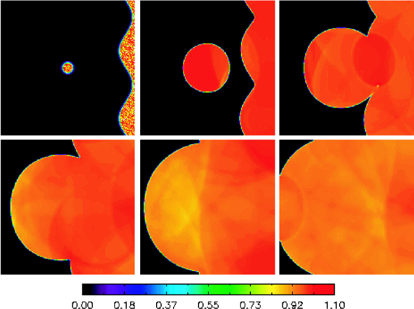
Figure 9: Contour plots of the scalar field for an interacting perturbed plane and a smaller nucleating bubble in the deflagration limit with $T=0.9T_{c}$ and $\kappa=7.0$. Results are shown at times 0, 2.0, 4.1, 6.1, 8.1, and $10.2\times 10^{-21}$ s for grid dimensions of 1000 fm along both the $x$ and $y$ axes. All images are scaled to the same global color map scheme.

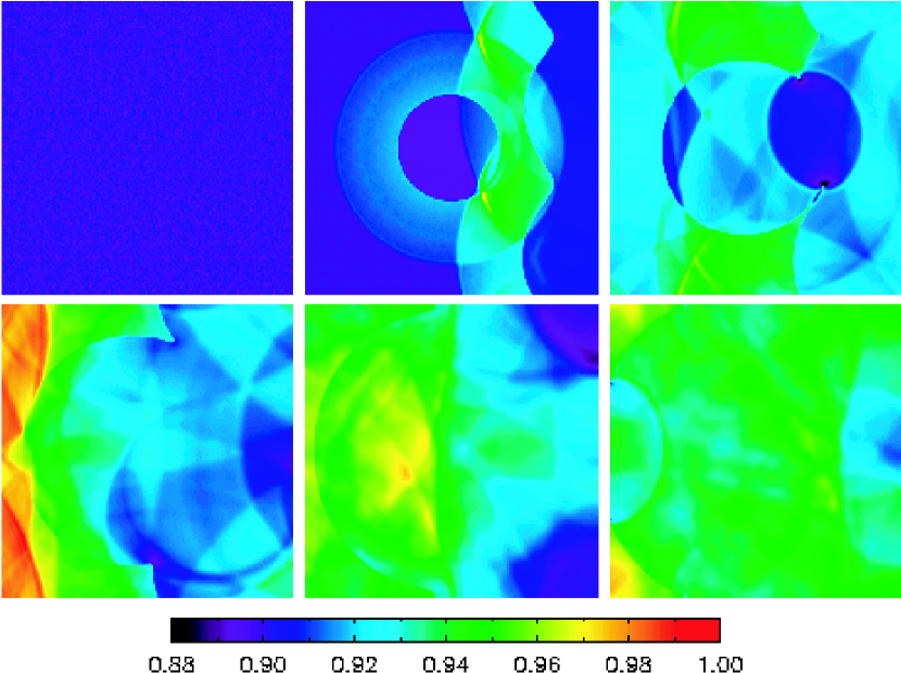
Figure 10: As Figure 9, but showing the fluid temperature in units of the critical temperature ($T_{c}=1$) at the same corresponding times.

Figures 11 and 12 show the scalar field and temperature for run E up to time $t\approx 1.6t_{s}$ in the final image. In contrast to the deflagration results of Figures 9 and 10, these images exhibit more complex behavior. In particular, front collisions result in the continuous generation of coherent quark “nuggets” formed by the greater entropy heating of hadrons at shock contact regions, a result consistent with the one-dimensional calculations shown in Figure 4. The nuggets are generally formed over spatial scales set by the length of the thermal plateau separating the leading shock from the rarefaction wave (or equivalently by the coherence length of the hot leading phase of hadrons at the time of impact). This, in turn, is set by the mean free path between hadron bubbles or thermal discontinuities and the strength of the detonation front which sets the relative velocity difference between the shock and rarefaction fan. A simple dimensional argument suggests that maximum quark fragment sizes are expected to be of order $\delta l=\delta v\delta t\sim L/6$, or roughly 16% of the box size. In this crude estimate we assume for the velocity difference determining the plateau width $\delta v\sim c_{s}/3$ as found in the 1D numerical solutions, the time between collisions $\delta t\sim L/(2c_{s})$, and $L/2$ represents the free path length between bubbles in this simulation. The numerical results find quark regions ranging in size from the smallest resolved scale of approximately one fermi determined by the cell size, up to a few hundred fermi, consistent with the above expected result. Once formed, the nuggets eventually decay away over roughly a sound crossing time due to adiabatic cooling and the generation of rarefaction waves at phase boundaries. Nugget shapes are generally determined by local shock and phase front geometries, but invariably they tend to become more spherical as the droplets decay and surface tension effects become significant enough to help erase surface perturbations.

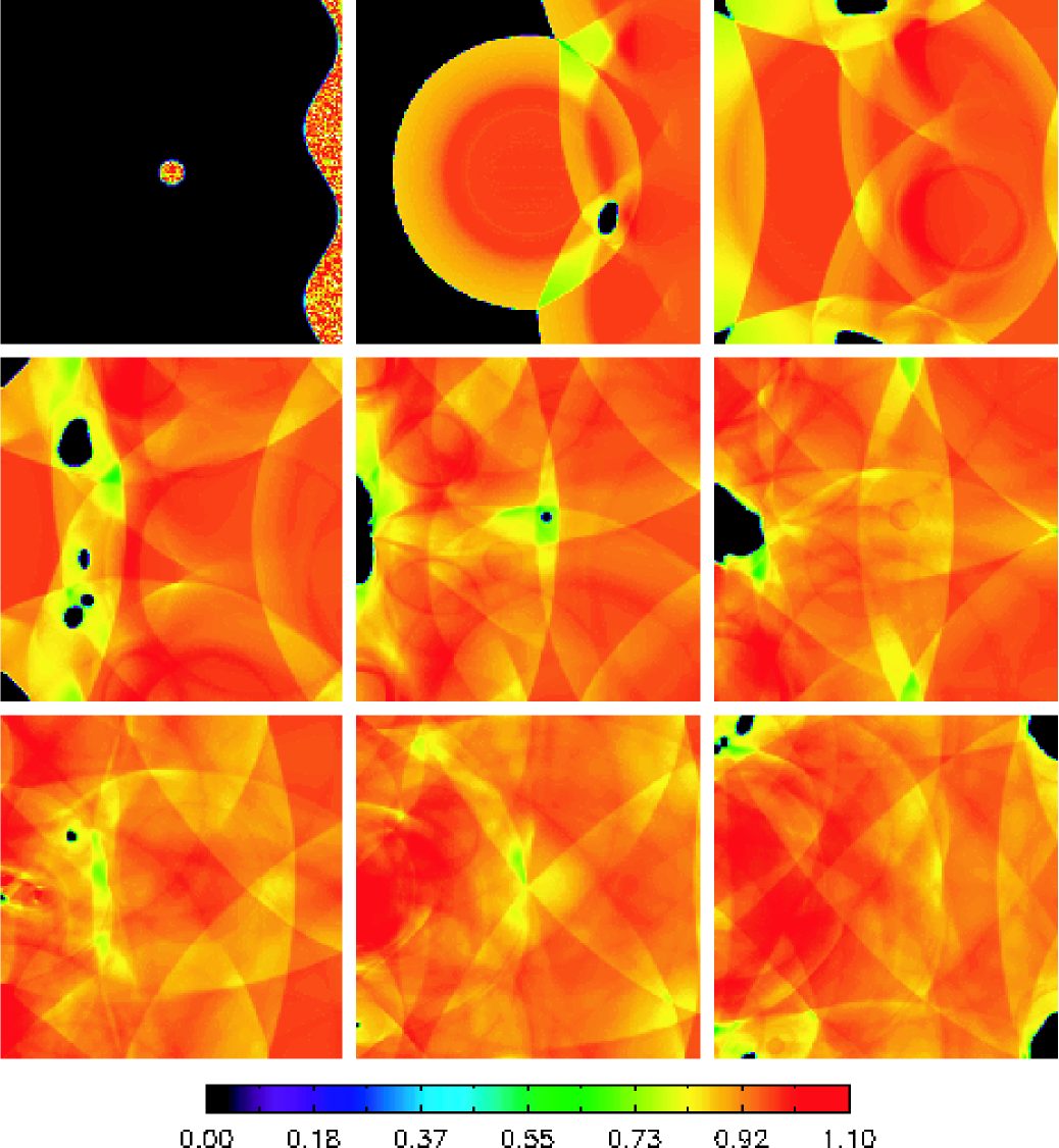
Figure 11: Contour plots of the scalar field for an interacting perturbed plane and a smaller nucleating bubble in the detonation limit with $T=0.9T_{c}$ and $\kappa=0.5$. Results are shown at times 0, 1.4, 2.7, 4.1, 5.4, 6.1, 7.1, 8.1, and $9.1\times 10^{-21}$ s, on a grid of dimension 1000 fm in each direction.

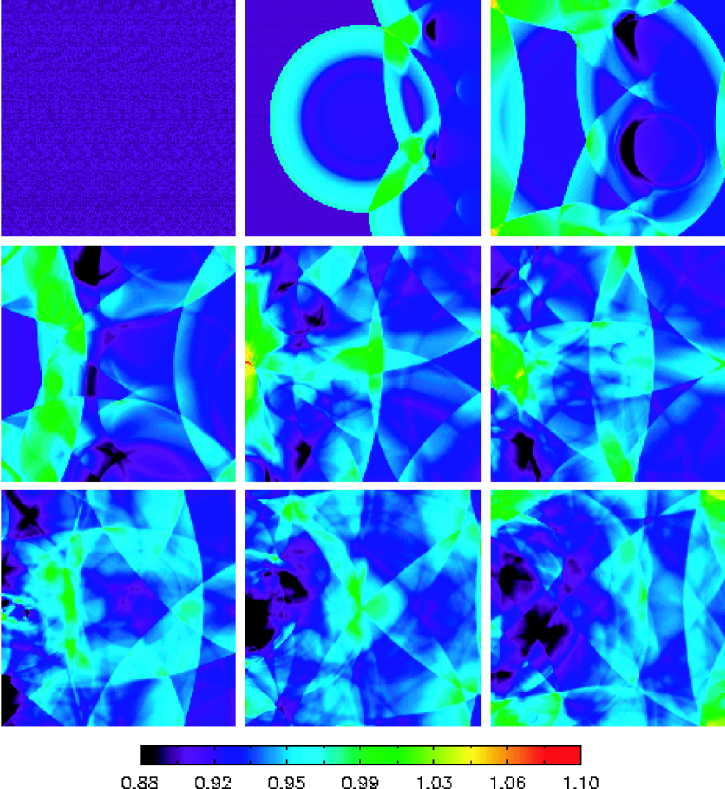
Figure 12: As Figure 11, but showing the temperature.

A final calculation presented here is run F, which considers the interaction of a deflagrating system with a detonation front nucleating from two different regions in space out of thermal equilibrium. The parameters are the same as those used in the one-dimensional calculations of Figure 5 in section IV.2, but we also introduce a phase shift of $\pi/2$ between the two fronts along the transverse direction. Equal grid spacing is used in the two dimensions here, but with four times as many zones in the direction perpendicular to the fronts. The physical size of the grid is set to $1806.1\times 451.53$ fm and resolved by $2048\times 512$ zones, chosen as a reasonable balance between resolution and run time. The physical run time of the final displayed image is $t=1.58t_{s}=1.65\times 10^{-20}$ s. The images in Figures 13 - 14 for this case show many of the same features exhibited by the interaction of two detonation fronts, in particular the decomposition of condensed hadrons into quark droplets or decaying nuggets at shock collisions. The spontaneously generated nugget regions remain (or become) regular during their lifetime, as do the phase boundaries of the larger initial phase fronts.

Another interesting feature found in this case is the deflagration ‘instability’ also noted in the one-dimensional results of Figure 5. Although precise quantification of thermal and kinematic states ahead and behind the accelerated phase front is difficult due to the multi-dimensional perturbations, the phase front is somewhat easier to characterize since perturbations are not as pronounced in $\phi$. The deflagration front at the left side, as measured halfway along the $y$-axis, is accelerated from an initial velocity of $v_{f}=0.35c_{s}=0.2$ to a supersonic speed of about $1.2c_{s}=0.68$ by the passage of a rarefaction wave generated at the thermal discontinuity. However, the accelerated front velocities measured along the top or bottom of the $y$-axis is smaller and closer to the one-dimensional result described in section IV.2. The midpoint of the phase front, which lags behind the mean front position as shown in Figure 13, thus undergoes a greater acceleration due to surface tension and mode dissipation effects. Also, transverse perturbations affect the flow of the hadron phase by ‘folding’ the cold phase into itself, creating hadron domains ahead of the main front which enclose decaying quark regions and eventually merge to effectively increase the front propagation velocity.

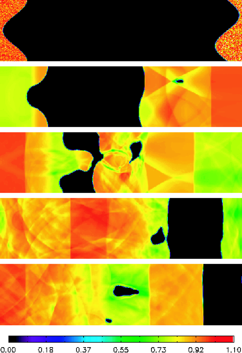
Figure 13: Contour plots of the scalar field for interacting perturbed plane fronts originating in two separate regions at different temperatures: a deflagration front at $T=0.9943T_{c}$ at the left end, and a detonation front propagating from the right end at $T=0.9T_{c}$. The dissipation constant is $\kappa=0.5$ everywhere on the grid of dimensions 1806.1$\times$451.53 fm, and the temperature discontinuity is initiated at the grid center along the $x$-axis. Results are shown at times 0, 4.0, 8.0, 12.5, and $16.5\times 10^{-21}$ s.

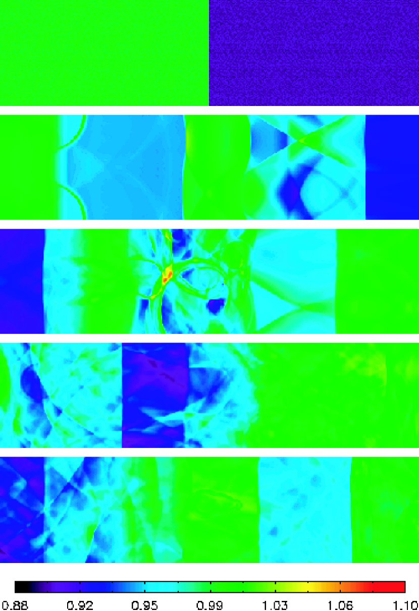
Figure 14: As Figure 13, but for the fluid temperature.

V Summary

We have performed both one- and two-dimensional numerical simulations of first order quark-hadron phase transitions in the early Universe. The primary goal of these studies was to explore the nature of the phase transitions beyond linear stability analysis, and determine if the interface regions between phases are inheritly stable or unstable when the full nonlinearities of the relativistic scalar field and hydrodynamic system of equations are accounted for. Whether interface boundaries are stable or unstable can have important consequences in our understanding of the standard picture of phase transitions and for the evolving baryon number density distribution, which we assume in this paper evolves hydrodynamically and coupled thermally and kinematically to a nonlinear scalar field with a quartic self-interaction potential. We used results from linear perturbation theory to define initial fluctuations on either side of the single phase front simulations, and evolved them numerically in time for both weak deflagrations and detonations. No evidence of unstable behavior is found in any of the isolated, single perturbed planar front cases we considered, despite the fact that the cases we chose to study are predicted to be unstable according to several linear analysis calculations. Indeed, the power spectra computed for the phase surface boundary and integrated fields behind the phase front all suggest that perturbations decay fairly rapidly, in fact much shorter then the growth time predicted by perturbation theory.

We are also motivated to determine whether phase mixing can occur through a turbulence-type mechanism triggered by shock proximity or the disruption of interfaces by pressure or shock waves. To investigate this scenario, we considered three cases: the first two involve the interaction of perturbed planar fronts with smaller nucleating hadron bubbles, one being entirely a deflagration scenario and the other a detonation; and a third case simulates the interaction between deflagration and detonation systems arising from two regions of space which have super-cooled to different temperatures and are thus out of initial thermal equilibrium. In the first case of planar-bubble deflagrations, the results are consistent with the standard picture of cosmological phase transitions in which hadron bubbles expand as spherical condensation fronts and undergo a process of regular (non-turbulent) coalescence, eventually leading to collapsing spherical quark droplets in a medium of hadrons. This behavior is generally supported also by the second case considering the interaction of multiple detonation bubbles. Although the evolutions in this second case are complicated by greater entropy heating from shock interactions, which contributes to the irregular destruction of hadrons and the creation of quark nuggets, the interfaces between phases remain coherent. Interface boundaries, including the original hadron bubbles as well as any newly formed quark nuggets, invariably evolve from complex distorted shapes (influenced by interacting multi-dimensional rarefaction waves, shocks, and phase fronts) to become more spherical as the nucleating regions expand, or as the quark nuggets collapse and surface tension becomes more important.

To summarize, although these calculations exhibit complex behavior, there are no signs of hydrodynamic mixing instabilities during this transition period, at least for the choice of parameters, scalar field interaction potential, equation of state, and grid resolutions investigated. Interfaces between quark and hadron phases remain regular, as perturbations along and across the phase boundaries are consistently damped out in time. Our results are thus generally consistent with the standard picture of cosmological phase transitions and with the conclusions of Huet et al. Huet et al. (1993), who suggest that electroweak transitions are stable according to linear analysis, even if similar definitive statements can not be made of quark-hadron transitions.

We also note an interesting deflagration ‘instability’ or acceleration mechanism evident in the third case for which we assume an initial thermal discontinuity in space separating different regions of nucleating hadron bubbles. The passage of a rarefaction wave through a slowly propagating deflagration can significantly accelerate the condensation process and the phase front to velocities near, or in excess of the sound speed. This suggests that if the universe super-cools at substantially different rates within causally connected domains, the dominant modes of condensation may be through supersonic detonations or fast moving (nearly sonic) deflagrations, assuming that conditions for triggering the instability are typical. A similar speculation was made by Kamionkowski and Freese Kamionkowski and Freese (1992) who suggested that deflagrations become unstable to perturbations and are converted to detonations over scales determined by linear theory and surface tension. In this scenario, instabilities distort the bubble shape, thereby increasing the surface area of the wall which accelerates the transition by increasing the rate of condensation and the effective velocity of expansion. However, for the calculations presented here, deflagrations are accelerated predominately not from turbulent mixing and surface distortion, but from enhanced super-cooling by rarefaction waves generated across thermal discontinuities. This effect can be significantly more pronounced in the presence of both longitudinal and transverse perturbations as we found by comparing one and two dimensional calculations with the same initial mean thermal states. In higher dimensions, the acceleration mechanism is exaggerated further by upwind phase mergers due to transverse flow, surface distortion, and mode dissipation effects, a combination that can result in supersonic front propagation speeds.